
A Convolutional Neural Network Model for Soil Temperature Prediction under Ordinary and Hot Weather Conditions: Comparison with a Multilayer Perceptron Model

 , ,
, ,  , ,
, , 
Abstract
1. Introduction
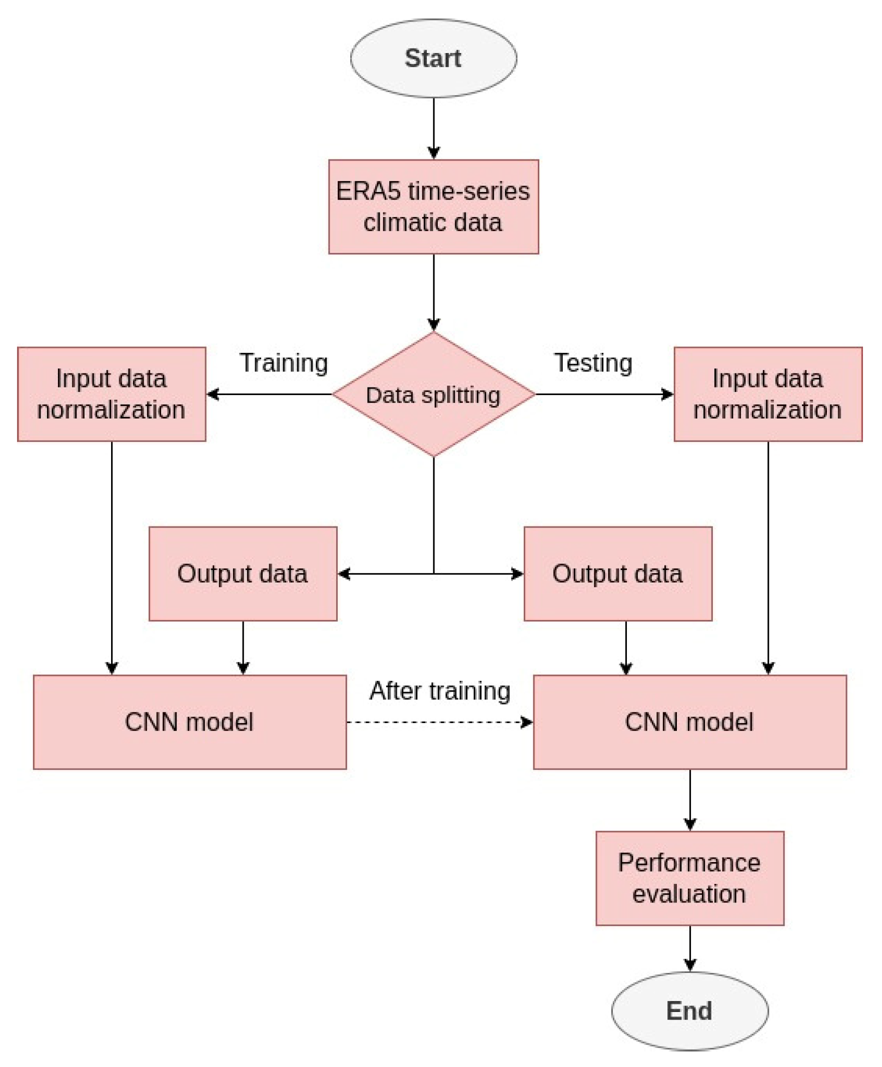
2. Methodology
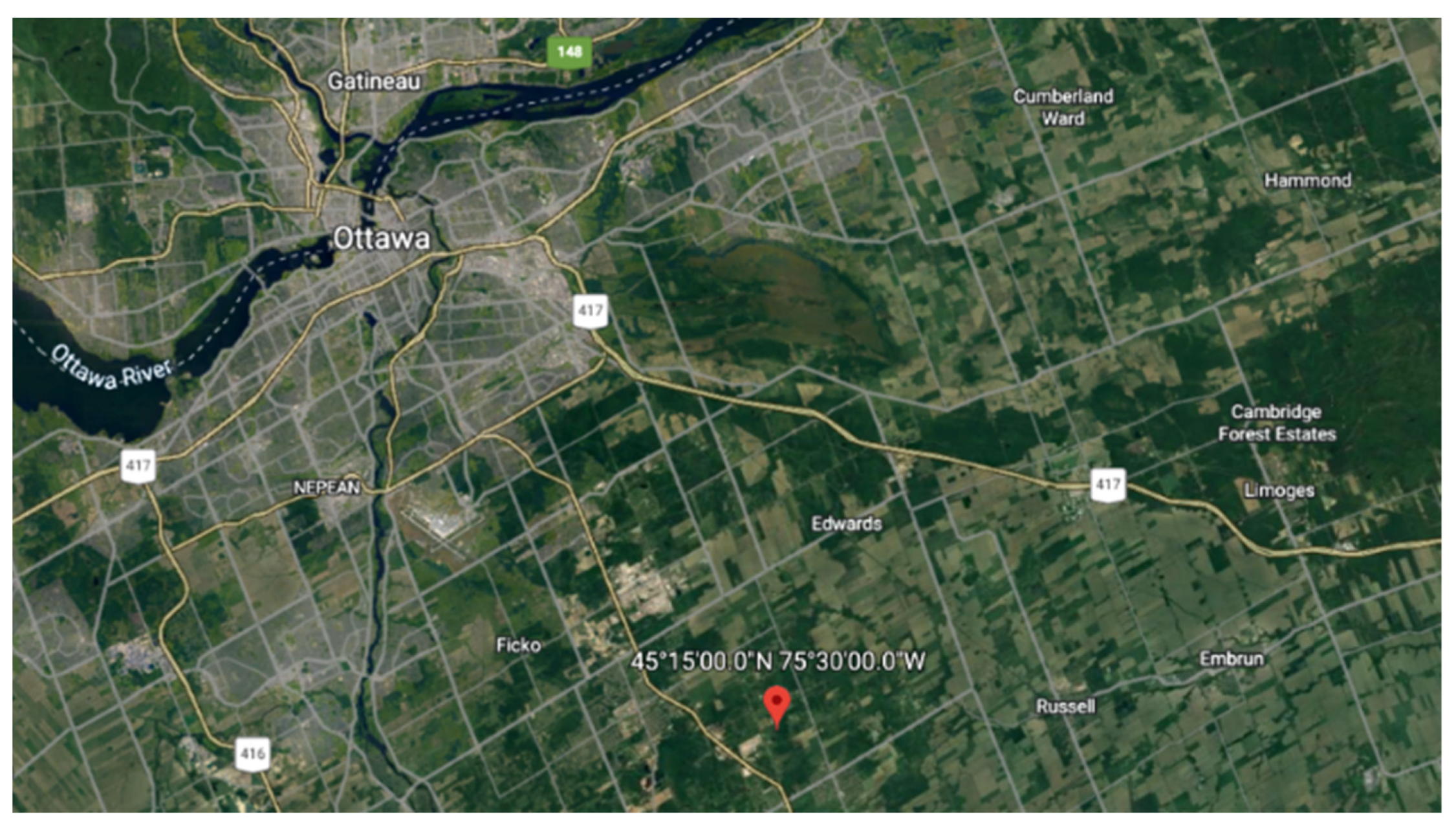
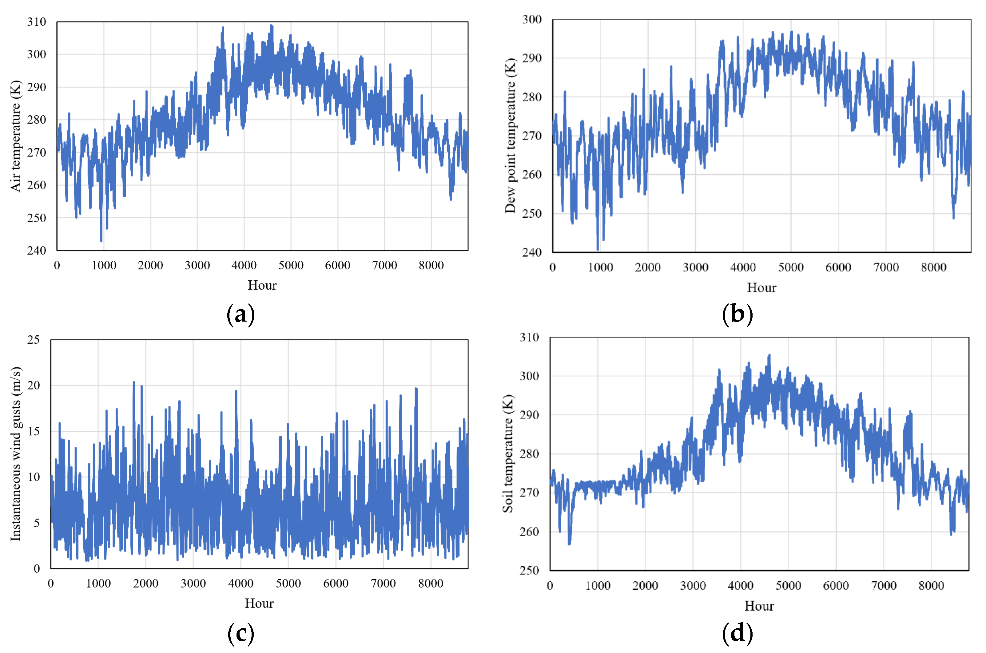
2.1. Study Area and Dataset
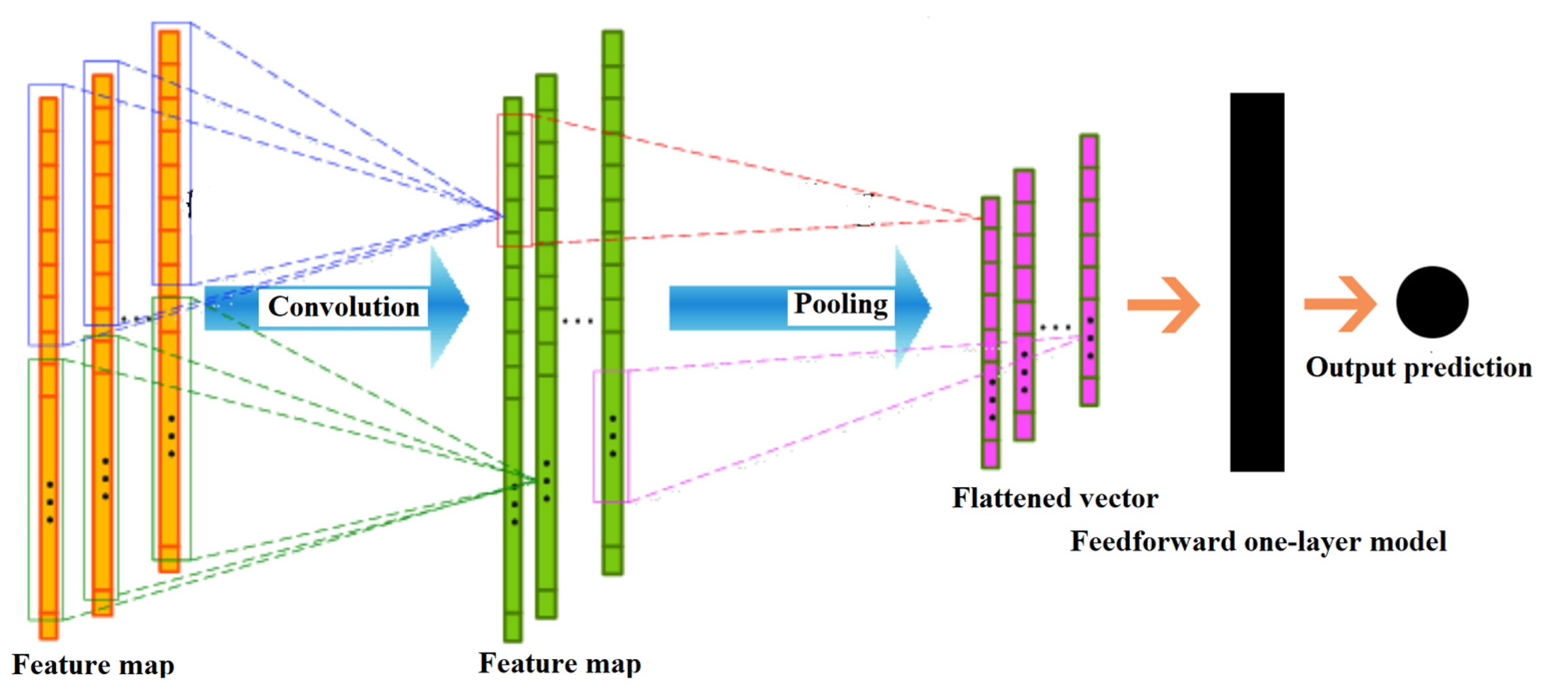
2.2. One-Dimensional CNN
2.3. Evaluation Metrics
3. Results and Discussion
3.1. 1D CNN Architecture
3.2. Climatic Features Significance in Soil Temperature Prediction
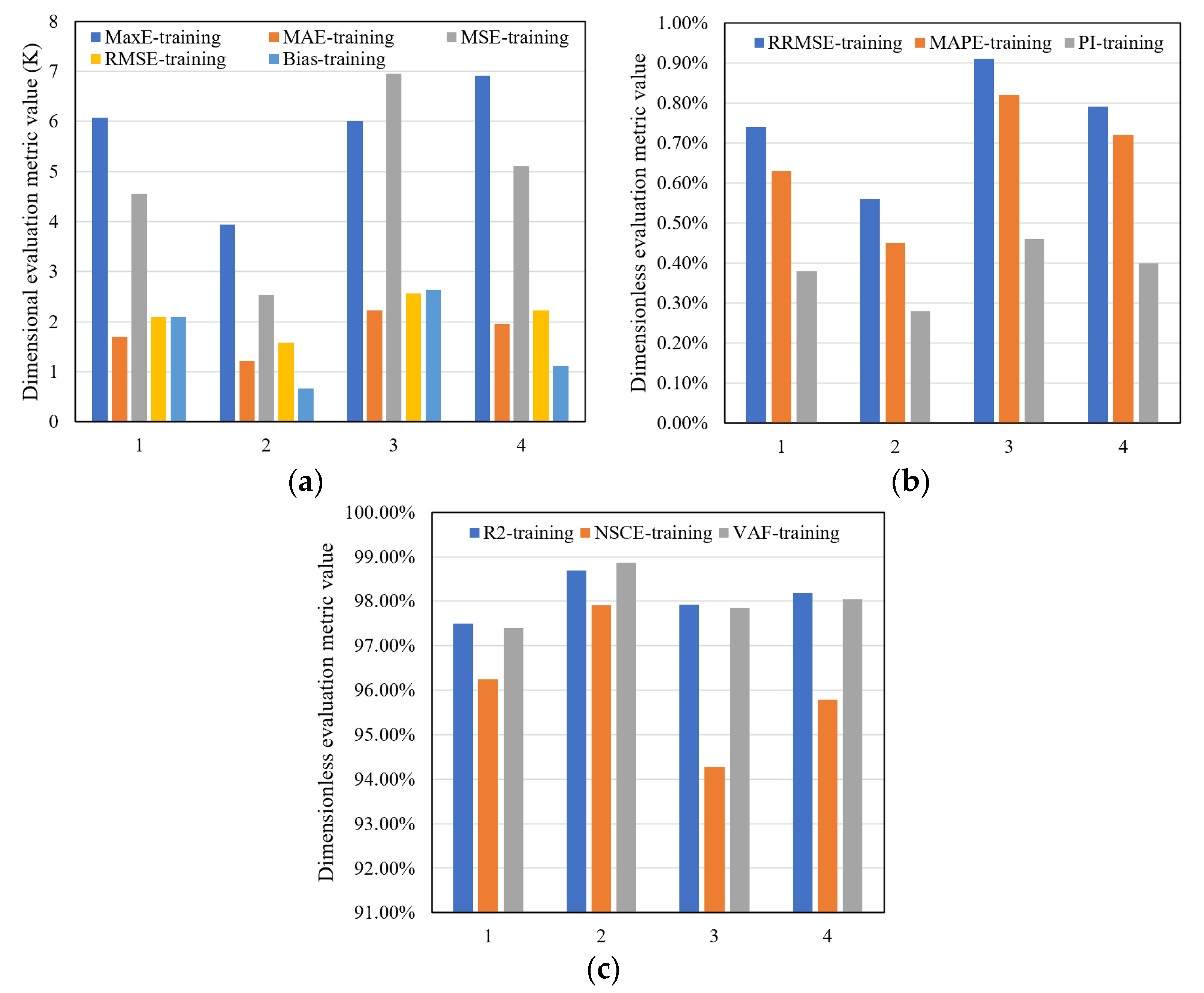
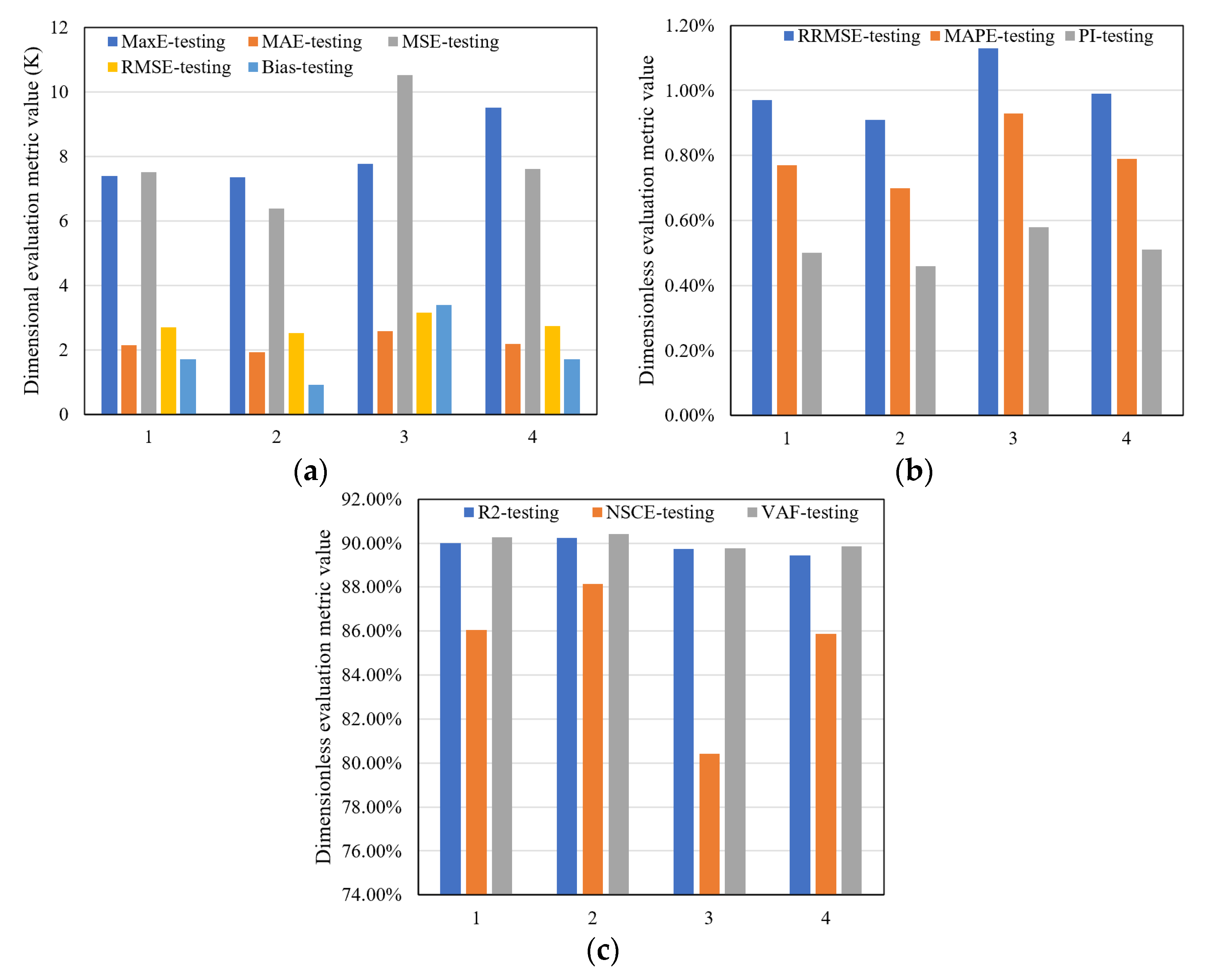
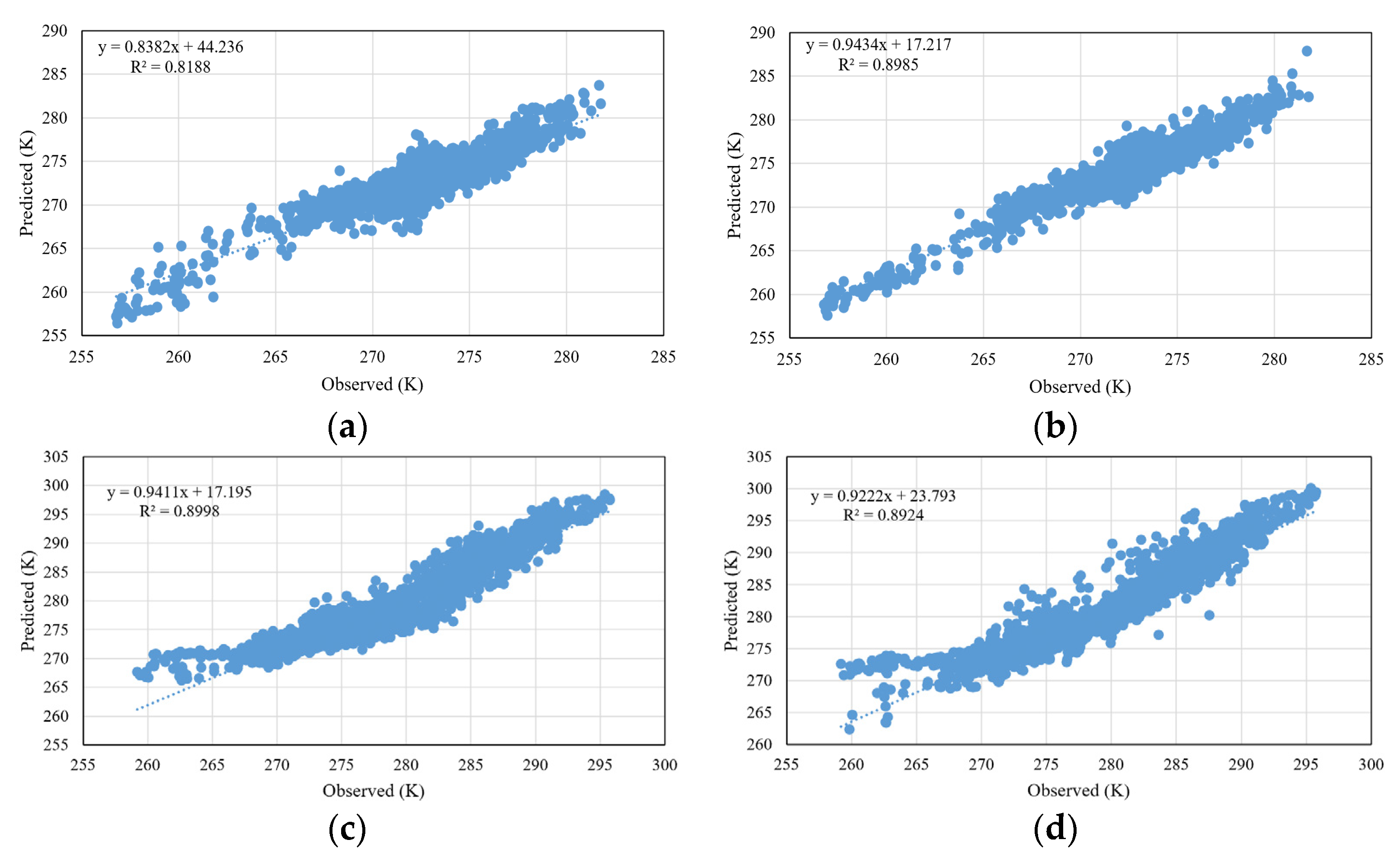
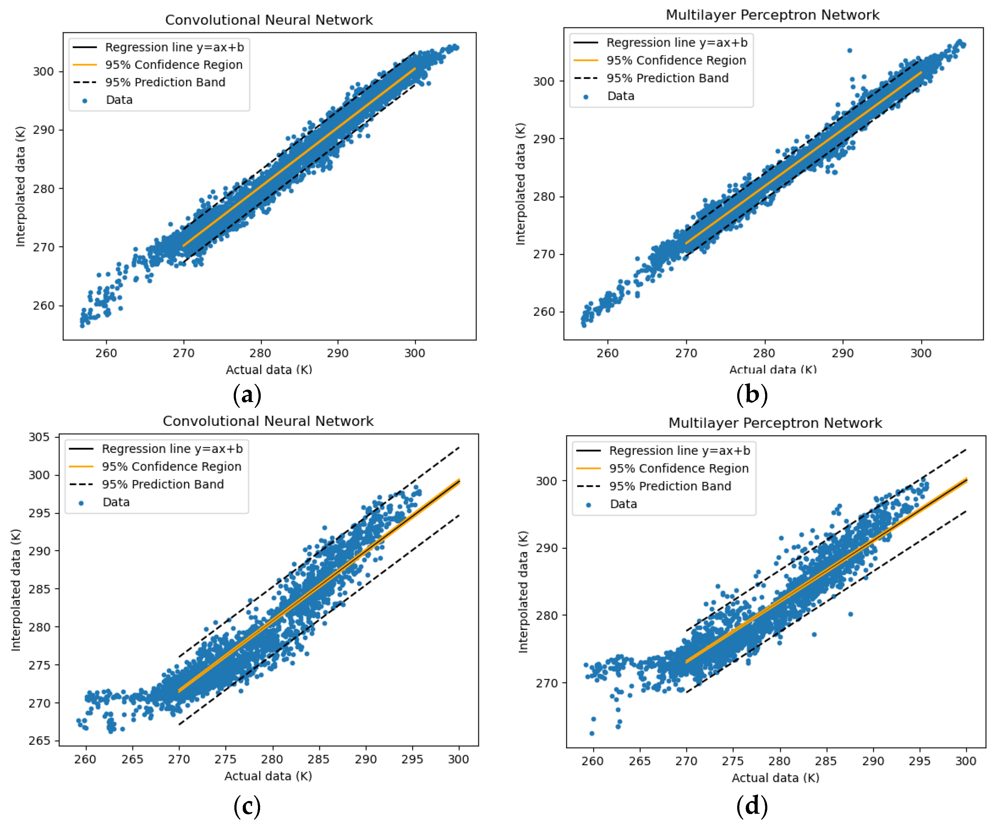
3.3. Performance Evaluation of the 1D CNN Model in Ordinary Weather Conditions
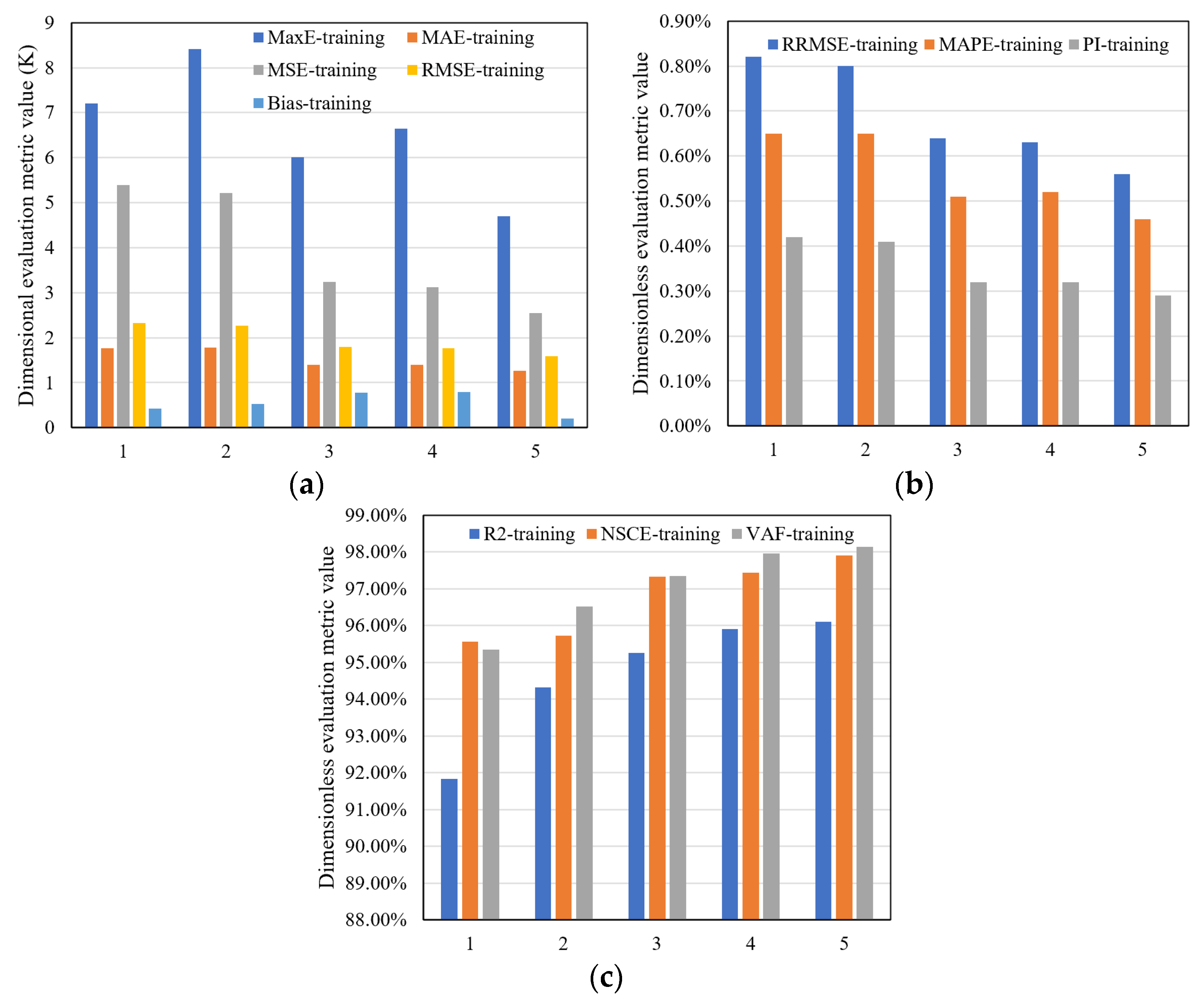
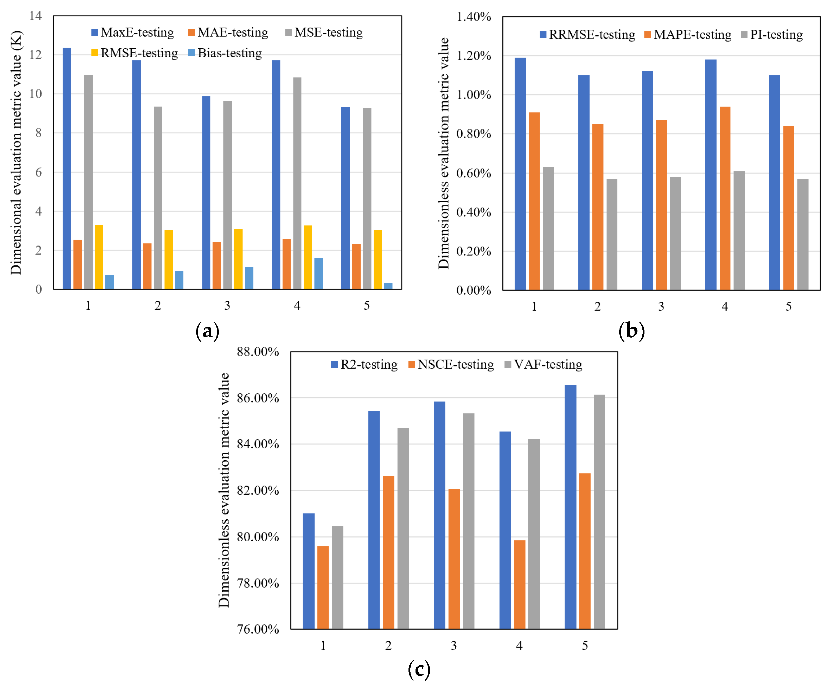
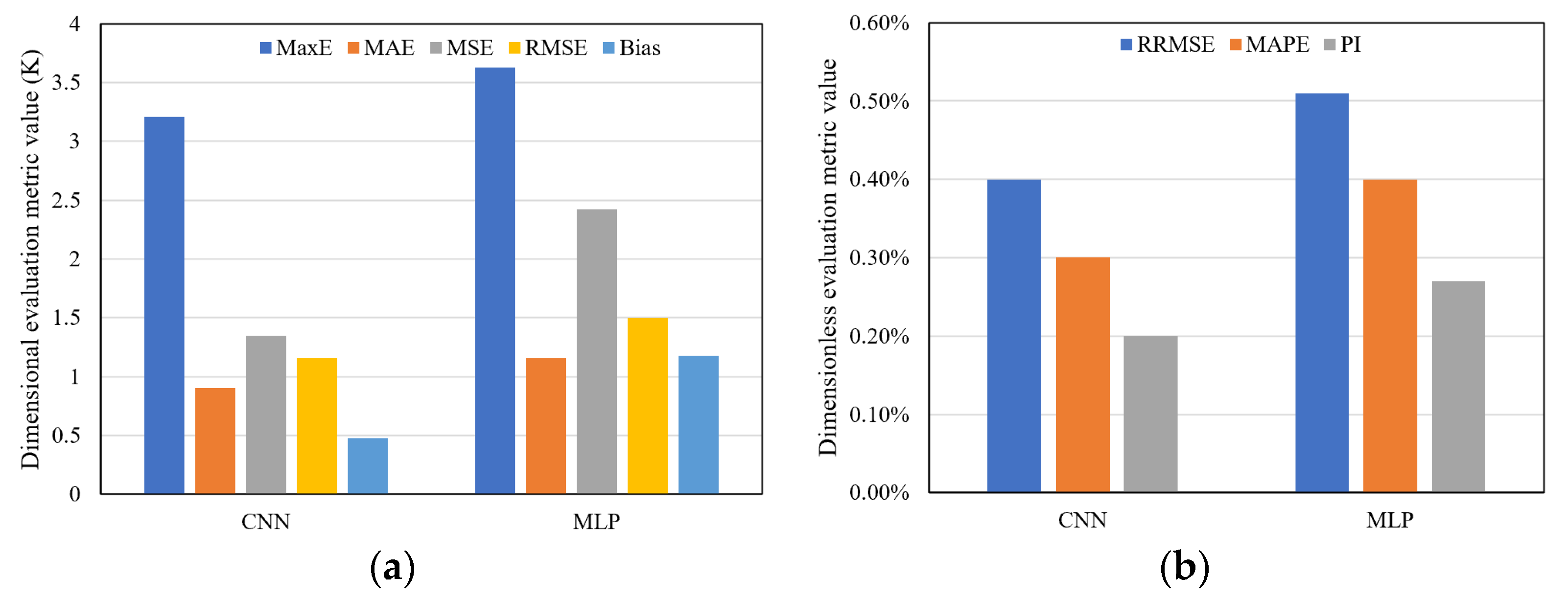
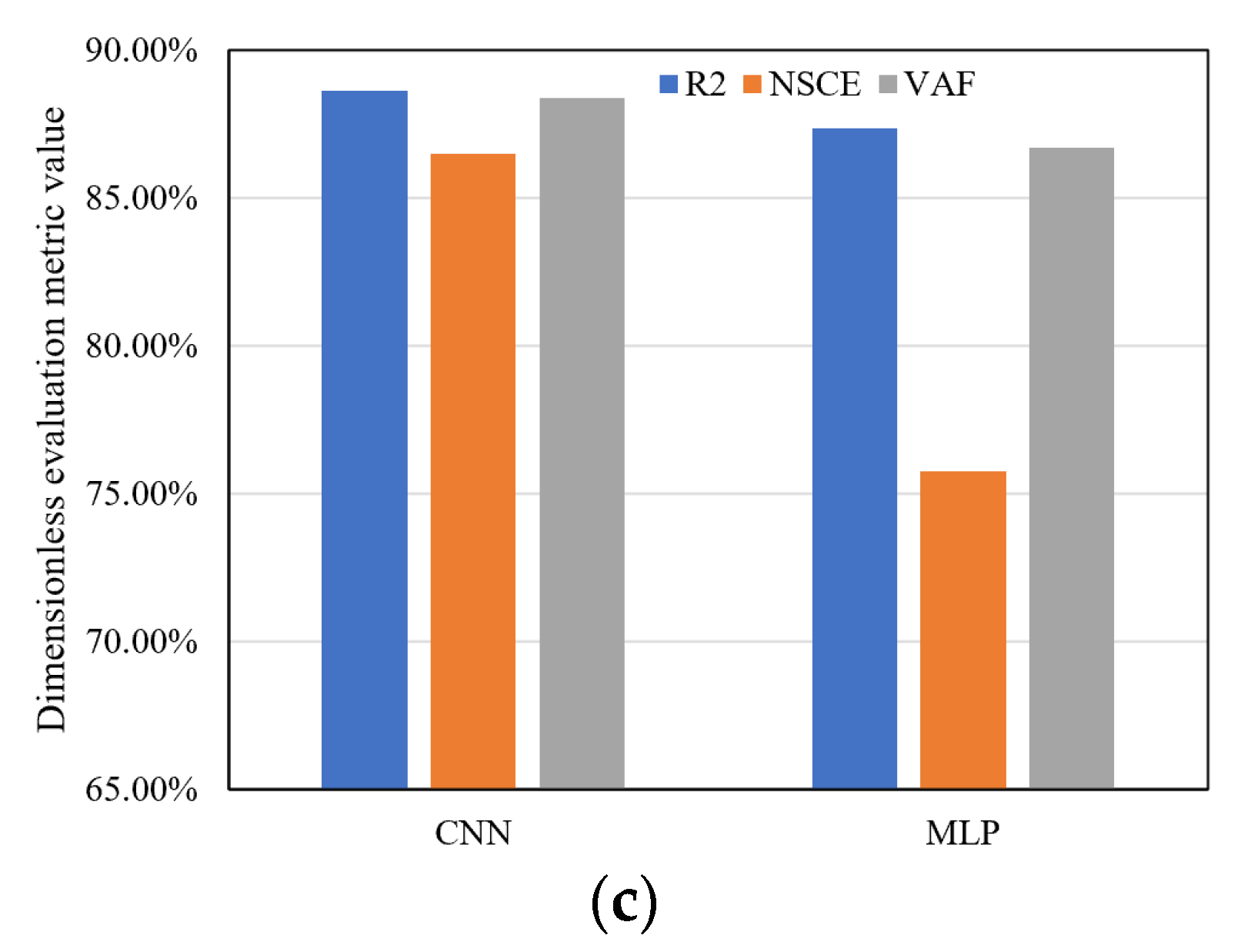
3.4. Performance Evaluation of the 1D CNN Model in Very Hot and Cold Weather Conditions
3.5. Capability of 1D CNN Model in Predicting the Daily Maximum Soil Temperature
4. Conclusions
Author Contributions
Funding
Data Availability Statement
Conflicts of Interest
References
- Lai, L.; Zhao, X.; Jiang, L.; Wang, Y.; Luo, L.; Zheng, Y.; Chen, X.; Rimmington, G.M. Soil respiration in different agricultural and natural ecosystems in an arid region. PLoS ONE 2012, 7, e48011. [Google Scholar] [CrossRef] [PubMed]
- Liang, L.; Riveros-Iregui, D.; Emanuel, R.; McGlynn, B. A simple framework to estimate distributed soil temperature from discrete air temperature measurements in data-scarce regions. J. Geophys. Res. Atmos. 2014, 119, 407–417. [Google Scholar] [CrossRef]
- Onwuka, B.; Mang, B. Effects of soil temperature on some soil properties and plant growth. Adv. Plants Agric. Res. 2018, 8, 34–37. [Google Scholar] [CrossRef]
- Yu, F.; Hao, H.; Li, Q. An ensemble 3D convolutional neural network for spatiotemporal soil temperature forecasting. Sustainability 2021, 13, 9174. [Google Scholar] [CrossRef]
- Araghi, A.; Mousavi-Baygi, M.; Adamowski, J.; Martinez, C.; van der Ploeg, M. Forecasting soil temperature based on surface air temperature using a wavelet artificial neural network. Meteorol. Appl. 2017, 24, 603–611. [Google Scholar] [CrossRef]
- Kisi, O.; Sanikhani, H.; Cobaner, M. Soil temperature modeling at different depths using neuro-fuzzy, neural network, and genetic programming techniques. Theor. Appl. Climatol. 2017, 129, 833–848. [Google Scholar] [CrossRef]
- Alizamir, M.; Kisi, O.; Ahmed, A.N.; Mert, C.; Fai, C.M.; Kim, S.; Kim, N.W.; El-Shafie, A. Advanced machine learning model for better prediction accuracy of soil temperature at different depths. PLoS ONE 2020, 15, e0231055. [Google Scholar] [CrossRef]
- Hao, H.; Yu, F.; Li, Q. Soil temperature prediction using convolutional neural network based on ensemble empirical mode decomposition. IEEE Access 2021, 9, 4084–4096. [Google Scholar] [CrossRef]
- Keshavarzi, A.; Sarmadian, F.; Omran, E.S.E.; Iqbal, M. A neural network model for estimating soil phosphorus using terrain analysis. Egypt. J. Remote Sens. Space Sci. 2015, 18, 127–135. [Google Scholar] [CrossRef]
- Zhang, Y. Soil temperature in Canada during the twentieth century: Complex responses to atmospheric climate change. J. Geophys. Res. 2005, 110, D03112. [Google Scholar] [CrossRef]
- Vandoorne, R.; Gräbe, P.J.; Heymann, G. Soil suction and temperature measurements in a heavy haul railway formation. Transp. Geotech. 2021, 31, 100675. [Google Scholar] [CrossRef]
- Feng, Y.; Cui, N.; Hao, W.; Gao, L.; Gong, D. Estimation of soil temperature from meteorological data using different machine learning models. Geoderma 2019, 338, 67–77. [Google Scholar] [CrossRef]
- Bonakdari, H.; Moeeni, H.; Ebtehaj, I.; Zeynoddin, M.; Mahoammadian, A.; Gharabaghi, B. New insights into soil temperature time series modeling: Linear or nonlinear? Theor. Appl. Climatol. 2019, 135, 1157–1177. [Google Scholar] [CrossRef]
- Zeynoddin, M.; Bonakdari, H.; Ebtehaj, I.; Esmaeilbeiki, F.; Gharabaghi, B.; Zare Haghi, D. A reliable linear stochastic daily soil temperature forecast model. Soil Tillage Res. 2019, 189, 73–87. [Google Scholar] [CrossRef]
- Mehdizadeh, S.; Fathian, F.; Safari, M.J.S.; Khosravi, A. Developing novel hybrid models for estimation of daily soil temperature at various depths. Soil Tillage Res. 2020, 197, 104513. [Google Scholar] [CrossRef]
- Zeynoddin, M.; Ebtehaj, I.; Bonakdari, H. Development of a linear based stochastic model for daily soil temperature prediction: One step forward to sustainable agriculture. Comput. Electron. Agric. 2020, 176, 105636. [Google Scholar] [CrossRef]
- Fradkov, A.L. Early history of machine learning. IFAC-PapersOnLine 2020, 53, 1385–1390. [Google Scholar] [CrossRef]
- Bochenek, B.; Ustrnul, Z. Machine learning in weather prediction and climate analyses-Applications and perspectives. Atmosphere 2022, 13, 180. [Google Scholar] [CrossRef]
- Abyaneh, H.Z.; Varkeshi, M.B.; Golmohammadi, G.; Mohammadi, K. Soil temperature estimation using an artificial neural network and co-active neuro-fuzzy inference system in two different climates. Arab. J. Geosci. 2016, 9, 377. [Google Scholar] [CrossRef]
- Citakoglu, H. Comparison of artificial intelligence techniques for prediction of soil temperatures in Turkey. Theor. Appl. Climatol. 2017, 130, 545–556. [Google Scholar] [CrossRef]
- Zhang, X.; Zhang, Q.; Zhang, G.; Nie, Z.; Gui, Z.; Que, H. A novel hybrid data-driven model for daily land surface temperature forecasting using long short-term memory neural network based on ensemble empirical mode decomposition. Int. J. Environ. Res. Public Health 2018, 15, 1032. [Google Scholar] [CrossRef] [PubMed]
- Delbari, M.; Sharifazari, S.; Mohammadi, E. Modeling daily soil temperature over diverse climate conditions in Iran-A comparison of multiple linear regression and support vector regression techniques. Theor. Appl. Climatol. 2019, 135, 991–1001. [Google Scholar] [CrossRef]
- Li, C.; Zhang, Y.; Ren, X. Modeling hourly soil temperature using deep BiLSTM neural network. Algorithms 2020, 13, 173. [Google Scholar] [CrossRef]
- Penghui, L.; Ewees, A.A.; Beyaztas, B.H.; Qi, C.; Salih, S.Q.; Al-Ansari, N.; Bhagat, S.K.; Yaseen, Z.M.; Singh, V.P. Metaheuristic optimization algorithms hybridized with artificial intelligence model for soil temperature prediction: Novel model. IEEE Access 2020, 8, 51884–51904. [Google Scholar] [CrossRef]
- Shamshirband, S.; Esmaeilbeiki, F.; Zarehaghi, D.; Neyshabouri, M.; Samadianfard, S.; Ghorbani, M.A.; Mosavi, A.; Nabipour, N.; Chau, K.W. Comparative analysis of hybrid models of firefly optimization algorithm with support vector machines and multilayer perceptron for predicting soil temperature at different depths. Eng. Appl. Comput. Fluid Mech. 2020, 14, 939–953. [Google Scholar] [CrossRef]
- Seifi, A.; Ehteram, M.; Nayebloei, F.; Soroush, F.; Gharabaghi, B.; Haghighi, A.T. GLUE uncertainty analysis of hybrid models for predicting hourly soil temperature and application wavelet coherence analysis for correlation with meteorological variables. Soft Comput. 2021, 25, 10723–10748. [Google Scholar] [CrossRef]
- Imanian, H.; Hiedra Cobo, J.; Payeur, P.; Shirkhani, H.; Mohammadian, A. A comprehensive study of artificial intelligence applications for soil temperature prediction in ordinary climate conditions and extremely hot events. Sustainability 2022, 14, 8065. [Google Scholar] [CrossRef]
- Shomron, G.; Weiser, U. Spatial correlation and value prediction in convolutional neural networks, IEEE Comput. Archit. Lett. 2019, 18, 10–13. [Google Scholar] [CrossRef]
- O’Gorman, P.A.; Dwyer, J.G. Using machine learning to parameterize moist convection: Potential for modeling of climate, climate change, and extreme events. J. Adv. Model. Earth Syst. 2018, 10, 2548–2563. [Google Scholar] [CrossRef]
- Huang, L.; Kang, J.; Wan, M.; Fang, L.; Zhang, C.; Zeng, Z. Solar radiation prediction using different machine learning algorithms and implications for extreme climate events. Front. Earth Sci. 2021, 9, 596860. [Google Scholar] [CrossRef]
- Araújo, A.D.S.; Silva, A.R.; Zárate, L.E. Extreme precipitation prediction based on neural network model-A case study for southeastern Brazil. J. Hydrol. 2022, 606, 127454. [Google Scholar] [CrossRef]
- Hersbach, H.; Bell, B.; Berrisford, P.; Biavati, G.; Horányi, A.; Muñoz Sabater, J.; Nicolas, J.; Peubey, C.; Radu, R.; Rozum, I.; et al. ERA5 Hourly Data on Single Levels from 1979 to Present. In Copernicus Climate Change Service (C3S) Climate Data Store (CDS); 2018. Available online: https://cds.climate.copernicus.eu/cdsapp#!/dataset/reanalysis-era5-single-levels?tab=overview (accessed on 21 November 2022).
- Google Maps. Available online: https://www.google.ca/maps/@45.3759264,-75.7182361,11.33z (accessed on 21 November 2022).
- Wang, X.; Li, W.; Li, Q. A new embedded estimation model for soil temperature prediction. Sci. Program. 2021, 2021, 5881018. [Google Scholar] [CrossRef]
- Kim, P. MATLAB Deep Learning: With Machine Learning, Neural Networks and Artificial Intelligence; Apress: Seoul, Republic of Korea, 2017; pp. 103–120. [Google Scholar]
- Gebrehiwot, A.; Hashemi-Beni, L.; Thompson, G.; Kordjamshidi, P.; Langan, T. Deep convolutional neural network for flood extent mapping using unmanned aerial vehicles data. Sensors 2019, 19, 1486. [Google Scholar] [CrossRef]
- Xu, D.; Zhang, S.; Zhang, H.; Mandic, D.P. Convergence of the RMSProp deep learning method with penalty for nonconvex optimization. Neural Netw. 2021, 139, 17–23. [Google Scholar] [CrossRef]
- Imanian, H.; Shirkhani, H.; Mohammadian, A.; Hiedra Cobo, J.; Payeur, P. Spatial interpolation of soil temperature and water content in the land-water interface using artificial intelligence. Water 2023, 15, 473. [Google Scholar] [CrossRef]
- Tüysüzoglu, G.; Birant, D.; Kiranoglu, V. Soil temperature prediction via self-training: Izmir case. J. Agric. Sci. 2022, 28, 47–62. [Google Scholar] [CrossRef]
- Bayatvarkeshi, M.; Bhagat, S.K.; Mohammadi, K.; Kisi, O.; Farahani, M.; Hasani, A.; Deo, R.; Yaseen, Z.M. Modeling soil temperature using air temperature features in diverse climatic conditions with complementary machine learning models. Comput. Electron. Agric. 2021, 185, 106158. [Google Scholar] [CrossRef]
- Samadianfard, S.; Ghorbani, M.A.; Mohammadi, B. Forecasting soil temperature at multiple-depth with a hybrid artificial neural network model coupled-hybrid firefly optimizer algorithm. Inf. Process. Agric. 2018, 5, 465–476. [Google Scholar] [CrossRef]


| (a) | |||||||
| Training | MaxE | MAE | MSE | RMSE | NRMSE | RRMSE | MAPE |
| Three layers, 64, 32, 16 kernels | 3.94 | 1.22 | 2.54 | 1.58 | 3.25% | 0.56% | 0.45% |
| Two layers, 256, 128 kernels | 4.70 | 1.27 | 2.54 | 1.59 | 3.27% | 0.56% | 0.46% |
| Testing | MaxE | MAE | MSE | RMSE | NRMSE | RRMSE | MAPE |
| Three layers, 64, 32, 16 kernels | 7.35 | 1.93 | 6.37 | 2.52 | 6.90% | 0.91% | 0.70% |
| Two layers, 256, 128 kernels | 9.33 | 2.34 | 9.28 | 3.04 | 8.32% | 1.10% | 0.84% |
| (b) | |||||||
| Training | R2 | NSCE | VAF | AIC | PI | ||
| Three layers, 64, 32, 16 kernels | 98.69% | 97.91% | 98.87% | 48368.13 | 0.28% | ||
| Two layers, 256, 128 kernels | 96.10% | 97.90% | 98.14% | 51884.45 | 0.29% | ||
| Testing | R2 | NSCE | VAF | AIC | PI | ||
| Three layers, 64, 32, 16 kernels | 90.25% | 88.14% | 90.42% | 24535.60 | 0.46% | ||
| Two layers, 256, 128 kernels | 86.54% | 82.73% | 86.13% | 25673.20 | 0.57% | ||
| MAE | MSE | RMSE | NRMSE (%) | RRMSE (%) | MAPE (%) | |
|---|---|---|---|---|---|---|
| All features included | 1.93 | 6.37 | 2.52 | 6.90 | 0.91 | 0.70 |
| Without precipitation | 2.52 (30.57%) | 10.08 (58.24%) | 3.10 (23.02%) | 8.49 (23.04%) | 1.12 (23.08%) | 0.91 (30.00%) |
| Without surface pressure | 2.23 (15.54%) | 8.15 (27.94%) | 2.83 (12.30%) | 7.73 (12.03%) | 1.02 (12.09%) | 0.81 (15.71%) |
| Without evaporation | 2.05 (6.22%) | 7.11 (11.62%) | 2.66 (5.56%) | 7.29 (5.65%) | 0.96 (5.49%) | 0.74 (5.71%) |
| Without wind gust | 2.12 (9.84%) | 7.81 (22.61%) | 2.77 (9.92%) | 7.57 (9.71%) | 1.00 (9.89%) | 0.77 (10.00%) |
| Without dewpoint temperature | 2.38 (23.32%) | 8.88 (39.40%) | 2.97 (17.86%) | 8.13 (17.83%) | 1.07 (17.58%) | 0.86 (22.86%) |
| Without surface solar radiation | 2.25 (16.58%) | 8.41 (32.03%) | 2.89 (14.68%) | 7.93 (14.93%) | 1.04 (14.29%) | 0.81 (15.71%) |
| Without surface thermal radiation | 1.94 (0.52%) | 6.53 (2.51%) | 2.55 (1.19%) | 6.98 (1.16%) | 0.92 (1.10%) | 0.70 (0.00%) |
| Without air temperature | 2.72 (40.93%) | 12.06 (89.32%) | 3.45 (36.90%) | 9.45 (36.96%) | 1.24 (36.26%) | 0.98 (40.00%) |
| (a) | |||||||
| Training | MaxE | MAE | MSE | RMSE | NRMSE | RRMSE | MAPE |
| CNN | 3.94 | 1.22 | 2.54 | 1.58 | 3.25% | 0.56% | 0.45% |
| MLP | 5.29 | 1.49 | 3.24 | 1.79 | 3.66% | 0.63% | 0.55% |
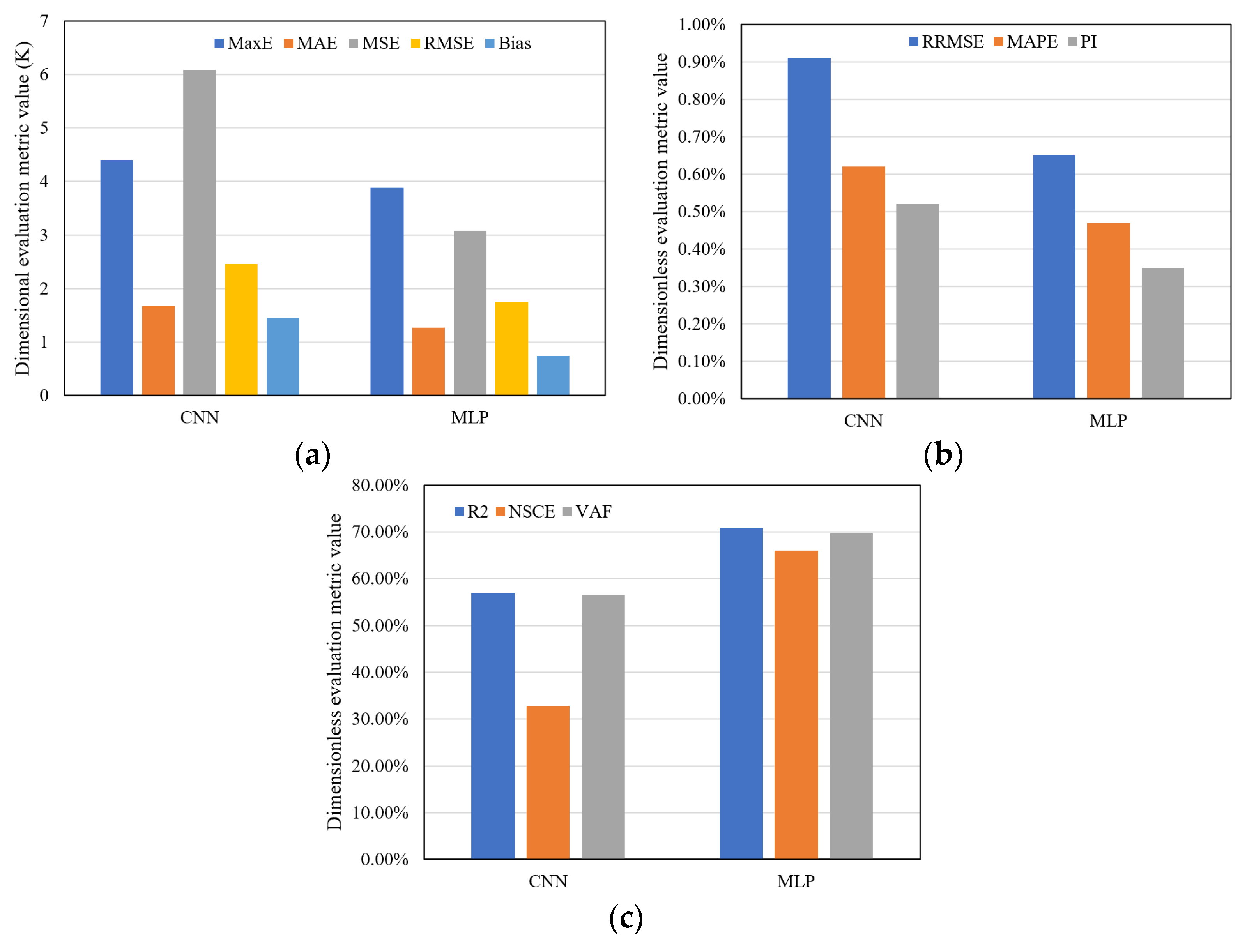
| Testing | MaxE | MAE | MSE | RMSE | NRMSE | RRMSE | MAPE |
| CNN | 7.35 | 1.93 | 6.37 | 2.52 | 6.90% | 0.91% | 0.70% |
| MLP | 8.87 | 2.03 | 7.49 | 2.72 | 7.43% | 0.98% | 0.73% |
| (b) | |||||||
| Training | bias | R2 | NSCE | VAF | AIC | PI | |
| CNN | 0.66 | 98.69% | 97.91% | 98.87% | 48368.13 | 0.28% | |
| MLP | 1.82 | 98.69% | 97.33% | 98.63% | 49476.55 | 0.32% | |
| Testing | bias | R2 | NSCE | VAF | AIC | PI | |
| CNN | 0.91 | 90.25% | 88.14% | 90.42% | 24535.60 | 0.46% | |
| MLP | 2.12 | 89.11% | 86.07% | 89.48% | 24748.12 | 0.50% | |
| Testing Phase | MaxE | MSE | RMSE | NRMSE | RRMSE | R2 | VAF | PI |
|---|---|---|---|---|---|---|---|---|
| CNN | 7.35 | 6.37 | 2.52 | 6.90% | 0.91% | 90.25% | 90.42% | 0.46% |
| RF | 11.63 | 6.43 | 2.54 | 6.93% | 0.91% | 88.19% | 88.78% | 0.46% |
| SVR | 12.11 | 7.47 | 2.73 | 7.48% | 0.94% | 86.28% | 88.86% | 0.48% |
| (a) | |||||||
| Phase | MaxE | MAE | MSE | RMSE | NRMSE | RRMSE | MAPE |
| Training | 3.62 | 2.10 | 6.54 | 2.48 | 5.49% | 0.87% | 0.73% |
| Testing | 5.72 | 3.58 | 19.23 | 4.35 | 13.31% | 1.55% | 1.28% |
| (b) | |||||||
| Phase | bias | R2 | NSCE | VAF | AIC | PI | |
| Training | 2.48 | 98.10% | 94.79% | 98.06% | 1658.96 | 0.43% | |
| Testing | 2.69 | 83.70% | 68.94% | 83.02% | 779.80 | 0.81% | |
Disclaimer/Publisher’s Note: The statements, opinions and data contained in all publications are solely those of the individual author(s) and contributor(s) and not of MDPI and/or the editor(s). MDPI and/or the editor(s) disclaim responsibility for any injury to people or property resulting from any ideas, methods, instructions or products referred to in the content. |
© 2023 by the authors. Licensee MDPI, Basel, Switzerland. This article is an open access article distributed under the terms and conditions of the Creative Commons Attribution (CC BY) license (https://creativecommons.org/licenses/by/4.0/).
Share and Cite
Farhangmehr, V.; Cobo, J.H.; Mohammadian, A.; Payeur, P.; Shirkhani, H.; Imanian, H. A Convolutional Neural Network Model for Soil Temperature Prediction under Ordinary and Hot Weather Conditions: Comparison with a Multilayer Perceptron Model. Sustainability 2023, 15, 7897. https://doi.org/10.3390/su15107897
Farhangmehr V, Cobo JH, Mohammadian A, Payeur P, Shirkhani H, Imanian H. A Convolutional Neural Network Model for Soil Temperature Prediction under Ordinary and Hot Weather Conditions: Comparison with a Multilayer Perceptron Model. Sustainability. 2023; 15(10):7897. https://doi.org/10.3390/su15107897
Chicago/Turabian StyleFarhangmehr, Vahid, Juan Hiedra Cobo, Abdolmajid Mohammadian, Pierre Payeur, Hamidreza Shirkhani, and Hanifeh Imanian. 2023. "A Convolutional Neural Network Model for Soil Temperature Prediction under Ordinary and Hot Weather Conditions: Comparison with a Multilayer Perceptron Model" Sustainability 15, no. 10: 7897. https://doi.org/10.3390/su15107897
APA StyleFarhangmehr, V., Cobo, J. H., Mohammadian, A., Payeur, P., Shirkhani, H., & Imanian, H. (2023). A Convolutional Neural Network Model for Soil Temperature Prediction under Ordinary and Hot Weather Conditions: Comparison with a Multilayer Perceptron Model. Sustainability, 15(10), 7897. https://doi.org/10.3390/su15107897