Article

A Hybrid Forecasting Model to Simulate the Runoff of the Upper Heihe River

1
School of Surveying and Land Information Engineering, Henan Polytechnic University, Jiaozuo 454000, China
2
Heihe Water Resources and Ecological Protection Research Center, Lanzhou 730030, China
*
Author to whom correspondence should be addressed.
Sustainability 2023, 15(10), 7819; https://doi.org/10.3390/su15107819
Submission received: 31 March 2023 / Revised: 3 May 2023 / Accepted: 8 May 2023 / Published: 10 May 2023

Abstract

:
River runoff simulation and prediction are important for controlling the water volume and ensuring the optimal allocation of water resources in river basins. However, the instability of medium- and long-term runoff series increases the difficulty of runoff forecasting work. In order to improve the prediction accuracy, this research establishes a hybrid deep learning model framework based on variational mode decomposition (VMD), the mutual information method (MI), and a long short-term memory network (LSTM), namely, VMD-LSTM. First, the original runoff data are decomposed into a number of intrinsic mode functions (IMFs) using VMD. Then, for each IMF, a long short-term memory (LSTM) network is applied to establish the prediction model, and the MI method is used to determine the data input lag time. Finally, the prediction results of each subsequence are reconstructed to obtain the final forecast result. We explored the predictive performance of the model with regard to monthly runoff in the upper Heihe River Basin, China, and compared its performance with other single and hybrid models. The results show that the proposed model has obvious advantages in terms of the performance of point prediction and interval prediction compared to several comparative models. The Nash–Sutcliffe efficiency coefficient (NSE) of the prediction results reached 0.96, and the coverage of the interval prediction reached 0.967 and 0.908 at 95% and 90% confidence intervals, respectively. Therefore, the proposed model is feasible for simulating the monthly runoff of this watershed.

1. Introduction

Runoff forecasting is an important component of hydrological research. The accurate simulation of runoff is important for research on water resource management, disaster monitoring, and the rational development and utilization of water resources [1,2]. Due to the effects of climate change and human activities, runoff sequences display obvious non-stationarity and complexity, which makes simulation and forecasting work difficult [3,4,5]. Therefore, establishing a high-precision runoff simulation model to effectively predict the changing trend of runoff has always been a hotspot in hydrological research.
As shown in Table 1, runoff forecasting models can generally be divided into process-driven and data-driven models (also known as black box models) [6]. Recently, with the emergence of big data, the increasing availability of hydrological and observation data, and the development of a large number of data mining algorithms, the interdisciplinary nature of this research is constantly expanding, and data-driven models are receiving increased attention [7,8,9,10]. The construction of a neural network, a kind of data-driven model, largely depends on the relationship between the input data and output features, thus providing a new research direction for runoff simulation [11,12,13]. As a kind of feedforward neural network, artificial neural networks (ANNs) are widely used in runoff forecasting due to their good ability to deal with nonlinear problems. Although their predictive performance is better than that of traditional distributed hydrological models, the neurons in each layer are independent of each other, and they cannot retain important information, thus having a limited ability to process time series data. The emergence of recurrent neural networks (RNNs) has solved these problems. The RNN realizes its network dynamic memory abilities through hidden layer cyclic connections. It can store previously obtained information, thereby realizing single- and multiple-step-ahead prediction functions [14].
Long short-term memory (LSTM) is a variant of an RNN that solves the gradient disappearance and gradient explosion problems of RNNs through a gating mechanism. LSTM can deal with complex correlation tasks between units in the sequence; it has received extensive attention in the field of hydrology [15,16,17]. Compared with traditional neural networks and physical models, LSTM models with measured data as the input have better performance. However, there is still room to improve their forecasting accuracy. To further improve prediction accuracy and efficiency, many scholars have focused their research on the optimization and improvement of the LSTM model architecture, such as by optimizing the model parameters or combining them with other models [18,19], etc. Many scholars have also discussed and analyzed the model’s data input and improved the prediction accuracy by seeking out more relevant input data [20].
The emergence of different signal decomposition methods, such as empirical mode decomposition, wavelet decomposition, and variational mode decomposition, has generated new bases for the prediction of non-stationary time series data [21,22,23]. Hybrid models that combine deep learning networks and various time–frequency decomposition methods have emerged and been continuously developed, largely solving the problem of non-stationary time series forecasting [24,25,26]. It is well known that the performance of deep learning model predictions largely depends on the inputs of the training samples. The time–frequency decomposition method decomposes the original runoff sequence into several components according to the central frequency so that each subsequence contains detailed information, which can be input into the deep learning model to improve its prediction accuracy. Muhammad S. et al. [27] developed a coupled artificial neural network model based on variational mode decomposition (VMD) and back-propagation (BP) to predict hydrological runoff, and the results were better than those obtained using a single BP model and a combined ensemble empirical mode decomposition back-propagation (EEMD-BP) model. Shuang et al. [28] researched the predictability of monthly streamflow using a support vector machine model coupled with discrete wavelet transform (DWT) and empirical mode decomposition (EMD). The results indicated that the EMD and DWT time series decomposition techniques improved the accuracy of the streamflow prediction. VMD is superior in center frequency aliasing and noise level control [29]. Therefore, in this study, it was combined with the LSTM model.
Traditional runoff forecasting studies only consider the accuracy of single-point forecasting results. Because of the non-stationarity and complexity of runoff series, the results of runoff forecasting are often unreliable and uncertain, and the fluctuations in runoff cannot be well understood based on only one fixed point value. Interval prediction has been further studied on the basis of point value prediction, and the range of forecasting error fluctuations is constrained based on confidence intervals to provide effective reference information [30,31]. In a sense, this approach reflects the uncertainty of prediction. The nonparametric kernel density estimation (KDE) method differs from the traditional parametric estimation model in that there is no assumption in advance that the error follows a given distribution, thus avoiding the problem of forecasting bias [32]. Interval forecasting has been widely used in hydrology and other fields. For example, Yang Xu. et al. [33] used rough set theory and the weighted Markov chain KDE method to forecast wind power probability intervals. The forecasting results displayed a higher coverage and a narrower average bandwidth than those of other methods. Du Bin. et al. [34] carried out interval forecasting of the urban water demand based on an optimized KDE distribution and an LSTM neural network and compared the results with those of other models. Zhang L. et al. [35] proposed a short-term wind speed probability density prediction framework based on quantile regression (QR) and KDE. The noise in the original wind speed sequence was mitigated by empirical modal decomposition (EMD). Research shows that the KDE method is suitable for interval forecasting.
In this paper, a combined VMD-LSTM deep learning model is constructed to simulate and forecast the monthly runoff at the Yingluoxia Hydrological Station in the upper Heihe River Basin, China; the data input lag time of the model is determined using a mutual information method. Additionally, on the basis of point forecasting, the KDE method is used to forecast runoff in intervals, and the range of the model forecasting error is simulated. Finally, the model accuracy is evaluated. This study aims to investigate the performance of the proposed model in predicting monthly runoff.

2. Materials and Methods

2.1. Study Area and Data

2.1.1. Study Area

The geographic coordinates of the Heihe River Basin are between 98° E~101°30′ E and 38° N~42° N, covering an area of approximately 142,900 km2 [36]. The upper reaches of the Heihe River, located in the Qilian Mountains at the northern foot of the Qinghai–Tibet Plateau, China, are situated in the Qilian Mountains–Qinghai Lake climatic zone, which is characterized by high precipitation, low evaporation, and low temperatures [37]. Affected by the climate and the flood season, with annual variations in flow, runoff is mainly concentrated from April to September, accounting for 80% of the annual flow; the runoff from October to March of the next year is relatively limited [38]. Notably, the runoff increases due to the rising temperatures from April to May, which result in snow and glacial melting [39]. Then, in the rainy season, with supplementary alpine ice and snow melt water, mountain runoff reaches a peak between July and August; runoff then decreases continuously after October, with decreasing temperatures and the weakening of the influence of warm and wet air flows [40]. The study area is shown in Figure 1.

2.1.2. Data

The data used in this study are monthly runoff data from the Yingluoxia Hydrological Station, situated in the upper reaches of the Heihe River, from 1982 to 2021; this study uses the monthly runoff from 1982 to 2011 as the training data set and the monthly runoff from 2012 and 2021 as the validation data set. The basic statistics of the runoff data from the Yingluoxia Hydrological Station are shown in Table 2. In Table 2, the overall runoff data display a highly skewed distribution, and the variation coefficient of monthly runoff data for each sample is approximately 0.8, which may affect the final runoff forecasting results to some extent. In order to improve the convergence rate of the model and ensure efficient training, the input data are normalized, and the output results are denormalized to obtain the actual predicted values. The normalization and inverse normalization formulas are as follows:
y * = y y min y max y min
Q = q ( y max y min ) + y min
where y * is a normalized runoff sequence; y is the original runoff sequence; y max and y min are the original maximum and minimum runoff values, respectively; q is the normalized prediction result; and Q is the inverse normalized prediction result.

2.2. Methodology

2.2.1. Variational Mode Decomposition

VMD is an adaptive non-recursive signal decomposition method for time–frequency distribution estimation [41,42]. The corresponding modal components of a non-stationary sequence are extracted by determining the center frequency and bandwidth of each component with a variational model, thus achieving the effective separation of each component [43]. The principle of this approach is described below. An original time series is decomposed into several IMFs using VMD, and the constrained variational formula for generating IMFs is:
{ Min { μ k } , { ω k } { k t [ ( δ ( t ) + j π t ) μ k ( t ) ] e j ω k t 2 2 } s . t . k μ k ( t ) = f ( t )
where k is the number of modes to be decomposed; { μ k } and { ω k } are the kth mode component and the center frequency, respectively, after decomposition; t is time; j2 = −1; δ is the Dirac function; and is a convolution operation.
By introducing the augmented Lagrange method, the constrained variational formula is updated to the following unconstrained formula:
L ( { μ k } , { ω k } , λ ) = α k t [ ( δ ( t ) + j π t ) μ k ( t ) ] e j ω k t 2 2 + f ( t ) k μ k ( t ) 2 2 + λ ( t ) , f ( t ) k μ k ( t )
where α is a secondary penalty factor that is mainly used to reduce noise interference; λ is a Lagrange multiplier; and a , b is the scalar product of a and b.
Then, by using alternating direction multiplication (ADMM) to iteratively update μ k n + 1 , ω k n + 1 and λ k n + 1 in the suboptimization sequence, the extreme point L is obtained, and the final formula is as follows:
μ ^ k n + 1 ( ω ) = f ^ ( ω ) i k μ ^ i ( ω ) + λ ^ ( ω ) 2 1 + 2 α ( ω ω k ) 2
ω k n + 1 = 0 ω | μ k n + 1 ( ω ) | 2 d ω 0 | μ k n + 1 ( ω ) | 2 d ω
λ ^ n + 1 ( ω ) = λ ^ n ( ω ) + τ [ f ^ ( ω ) k μ ^ k n + 1 ( ω ) ]
where ^ represents the Fourier transform and τ is the noise tolerance.
In this process, based on the error threshold ε , iterations are performed, and the results μ k and ω k are output based on Formula (8). If the appropriate conditions are not met, the process is repeated.
k μ k n + 1 μ k n 2 2 μ k n 2 2 < ε
where ε is the convergence tolerance.

2.2.2. Mutual Information

Mutual information can be used to reflect the degree of dependence or correlation between two variables. Mutual information is a quantitative concept based on information entropy, and it can be used to quantify the relationship between two random variables sampled at the same time [44,45]. The mutual information value I ( X , Y ) between X and Y can be expressed as:
I ( X , Y ) = i = 1 M j = 1 N P X Y ( x i , y j ) log P X Y ( x i , y j ) P 1 ( X = x i ) P 2 ( Y = y j )
where P ( x , y ) is the joint probability density function of x and y , and P x , P y are the marginal probability density functions of x and y , respectively.
MI is the amount of information used to evaluate the contribution of the occurrence of one event to the occurrence of another [46,47]. This approach can enhance feature selection if the MI values of all features and target features are calculated and then sorted to identify the features with the K highest MI values. Based on this method, MI can be used for feature selection and to identify inputs for deep learning [48].

2.2.3. LSTM

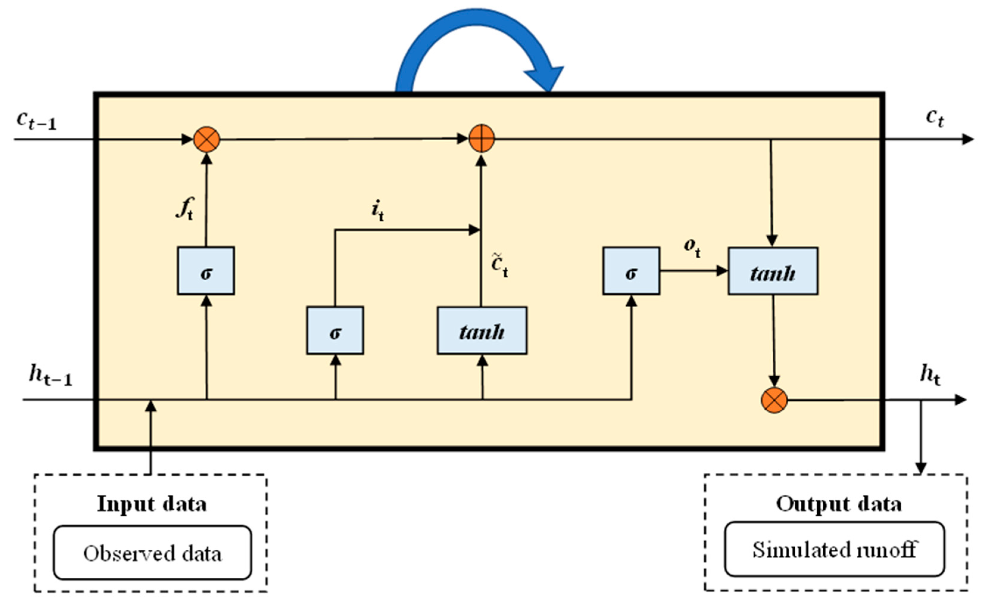
With the development of artificial neural networks, LSTM neural networks were developed to extract important information and discard less important information by simulating forgetting and remembering processes [49,50,51]. Compared with the RNNs, LSTMs have a more complex structure, which includes a forget gate, an input gate, and an output gate [51,52]. The structure of an LSTM cell is shown in Figure 2.
As an important link, the forget gate yields an output vector f t of 0~1 based on the previous output h t 1 (the implied state) and the current input x t through a sigmoid activation function. Specifically, the forgetting function of the human brain is simulated, and valuable information is filtered through the forget gate.
f t = σ ( W f · [ h t 1 , x t ] + b f )
The input gate i t is used to determine the extent to which the current input information x t should be added to the long-term memory information C t , and another candidate gate C t ~ is created by using the tan h function to calculate the unit status of the current input.
i t = σ ( W i · [ h t 1 , x t ] + b i )
C t ˜ = tan h ( W c · [ h t 1 , x t ] + b c )
In the neuron renewal stage, the information retained in the previous processing step and the current processing step is processed using the following formula, which is the key to simulating human memory. Throughout this step, C t is in a state of change and updated continuously with the applied neural network.
C t = f t c t 1 + i t C t ˜
At the output gate, the current output is assessed based on a sigmoid function and a tan h function to obtain the final output h t .
o t = σ ( W o · [ h t 1 , x t ] + b o )
h t = o t tan h ( C t )
where W f , W i , W c , and wo are the different weights derived from the forget, input, and output gates, respectively; b f , b i , b c and b o are the corresponding bias values; and f t , i t , and o t are the outputs of the activation function at time t.

2.2.4. Nonparametric Kernel Density Estimation

KDE is a classical nonparametric estimation method. Unlike in parametric estimation, the KDE distribution is used to obtain a PDF using only a given sample without assuming any prior distribution [53,54]. The values of the core homogeneity function at all sampling points are averaged to obtain the estimated density function. The KDE formula is as follows:
f ( x ) = 1 N h i = 1 N K ( x x i h )
where N is the sample length; h is the bandwidth used to adjust the width of the probability density curve; and K is the kernel function. There are various kernel functions that can be applied to KDE distributions, such as the Tophat function, the Gaussian kernel function, the trigonometric kernel function, the Epanechnikov function, and the exponential function [55,56]. Here, the commonly used Gaussian kernel function is selected.
K ( u ) = 1 2 π e u 2 2 , u R
The selection of the window frame h is the key step in KDE, and it directly affects the accuracy of the kernel estimation. According to previous scholars’ research [55,57], the optimal window width in the Gaussian kernel function can be expressed as:
h b e s t 1.06 σ ^ n 1 5

2.2.5. Evaluation of the Model’s Performance

Evaluating model performance is an important component of research. In this paper, the Nash–Sutcliffe efficiency (NSE), root mean square error (RMSE), and Pearson correlation coefficient (R) are used to evaluate the accuracy of model point prediction. The formulas are as follows:
N S E = 1 ( y i o b s y i p r e d ) 2 ( y i o b s y i ¯ ) 2
R M S E = i = 1 n ( y i o b s y i p r e d ) 2
R = i = 1 n ( y i o b s y o b s ¯ ) 2 i = 1 n ( y i p r e d y p r e d ¯ ) 2 i = 1 n ( y i o b s y o b s ¯ ) 2 i = 1 n ( y i p r e d y p r e d ¯ ) 2
where y i o b s is the measured runoff value at time i ; y i p r e d is the runoff forecast value at time i ; y o b s ¯ is the measured mean runoff; and y p r e d ¯ is the mean runoff prediction.
The Nash–Sutcliffe coefficient is a parameter used to evaluate the quality of a model, and it ranges from [− , 1]. This coefficient is generally used to verify the simulation results of hydrological models and other models. The forecasting results are acceptable when the NSE is greater than 0.5. The closer the NSE value is to 1, the better the prediction ability of the model is. The RMSE reflects the deviation between the measured and predicted values. The smaller the RMSE is, the higher the fitting degree of the model and the better the prediction effect. The Pearson correlation coefficient is a measure of the degree of linear correlation between two variables. It is usually expressed in terms of R, and the range of values is [–1,1]. The closer this parameter is to 1, the better the model performs.
The forecasting interval represents the range of change in forecasting results at a certain confidence level, which reflects the degree of uncertainty of the model forecasts [35,58]. In this paper, the model forecasts are assessed based on the PICP and average MPIW:
P I C P = 1 n i = 1 n p i , p i = { 0 1 y i o b s [ L i , U i ] y i o b s [ L i , U i ]
M P I W = 1 n i = 1 n ( U i L i )
where n is the forecast runoff quantity and p i indicates whether the measured runoff value in a given month i falls into the forecasting interval. If it falls within this interval, it is recorded as 1; otherwise, it is recorded as 0. L i and U i are the upper and lower bounds of the forecasting interval, respectively.
Interval coverage represents the overall ratio of runoff predictions that fall within the forecasting range. The larger the value is, the better the forecasting effect. Additionally, the smaller the average width of the interval is, the higher the clarity and accuracy of the results.

2.3. Model Implementation

2.3.1. Determining Network Parameters

The LSTM model used in this study is constructed using the TensorFlow and Keras deep learning frameworks. Hyperparameters can directly affect the performance of neural network structures, and selecting the hyperparameters of LSTM models remains a difficult task. Since there is no specific standard, the optimal model depth is selected through multiple experiments. After many experiments, the best model was set to consist of 3 hidden LSTM layers and a fully connected layer, where the hidden layers contain 100, 64, and 32 neurons. Zhang, J. et al. [59] have extensively tuned the architectural parameters of the LSTM model. We have adjusted and optimized the model parameters according to the constructed model. The maximum number of iterations, number of epochs, batch size, and activation function were set to 100, 36, and a rectified linear unit (ReLU), respectively, through trial and error. The dropout regularization method was used in the model to reduce overfitting, and the value of each LSTM layer was set to 0.3 [60]. In addition, stochastic gradient descent (SGD) was used to optimize the model parameters and minimize the loss function, and the learning rate was 0.005. SGD is a simple but highly effective method that is often used in deep learning model parameter optimization. The output value was a single variable, representing the runoff in the next month. In the learning process, the method used to update the parameters was the Adam random gradient descent method, and the loss function was based on the mean square error (MSE).
The number of time steps used in the model (that is, determining how much runoff in the previous month is used to predict the runoff in the next month) was determined based on an MI method. Taking the subsequence that needs to be predicted as the target variable, the MI value was calculated with different lag time subsequences. When the MI value is large, the current time series variable provides important information for the prediction of the target time series variable. Based on the monthly runoff at time t, the MI values at (t + 1), (t + 2), (t + 3), ⋯, and (t + n) are calculated. When the MI value reaches a maximum, the first n months starting from the current month are selected as months with characteristic inputs to predict the runoff in the next month. By using the MI method, we determined that the MI value of the runoff time series peaked when the lag time was 12 months; therefore, the model input time step was set to 12. The parameter inputs were consistent in the model training period and the verification period.

2.3.2. Process of Training the VMD-LSTM Model

Based on the VMD-LSTM model, the runoff at the Yingluoxia Hydrological Station in the upstream portion of the Heihe River Basin was forecast, the input delay was determined using the MI method for single-point forecasting, and the runoff sequence was continuously estimated with a nonparametric KDE algorithm, considering the errors between the point forecasting values and the actual measured values. Finally, an accuracy evaluation of the model forecasts was performed.
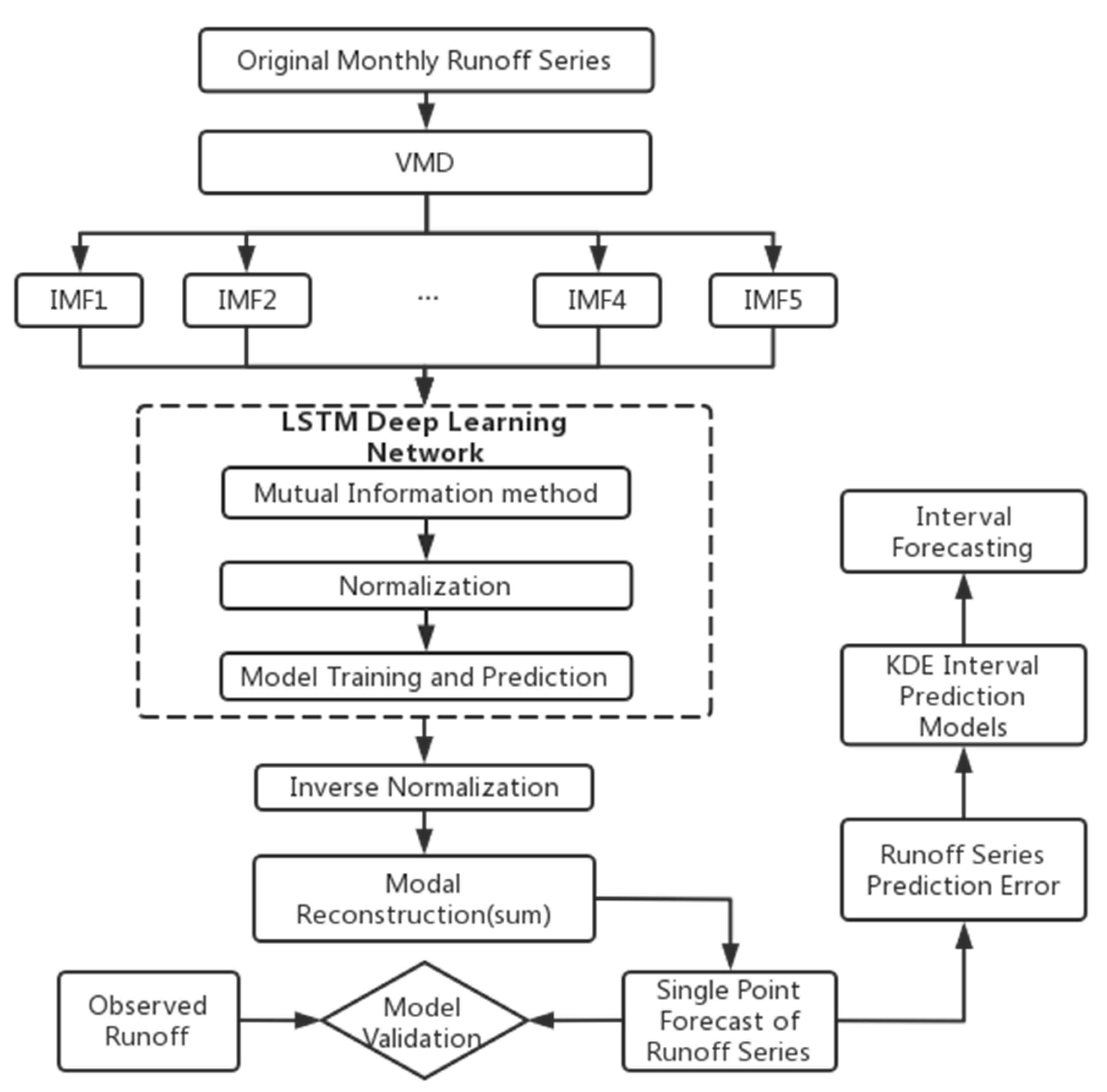
The VMD-LSTM model forecasting steps are as follows:
(1)
The required monthly runoff sample data are selected, and a model training set and a test set are established.
(2)
The VMD method is used to decompose the original runoff sequence to obtain several components, and each component and the original runoff sequence are normalized.
(3)
The MI method is used to determine the model input delay (in this paper, the time step), and each component is input into the LSTM model for prediction.
(4)
After the forecast is completed, the data are denormalized, and the prediction results for each mode component are combined to obtain the final runoff forecast sequence.
(5)
The runoff series forecasting error is calculated, the nonparametric KDE method is applied to estimate the runoff series interval, and the accuracy of prediction results is evaluated.
The specific forecasting process is as follows (Figure 3).

3. Results

3.1. Determination of the Number of VMD Components

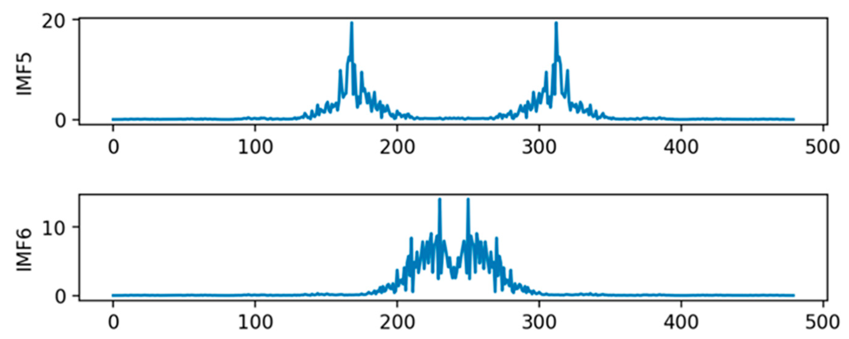
When the original monthly runoff data are decomposed using the VMD method, the number of modal IMFs considered affects the decomposition results [43,61]. When the number of decompositions is large, the center frequency of the subsequence may be difficult to discern. When the number of decompositions is small, some important information from the original runoff signal may be lost [24]. Therefore, the number of decompositions needs to be determined based on the center frequency of each component, as shown in the following figure (Figure 4).
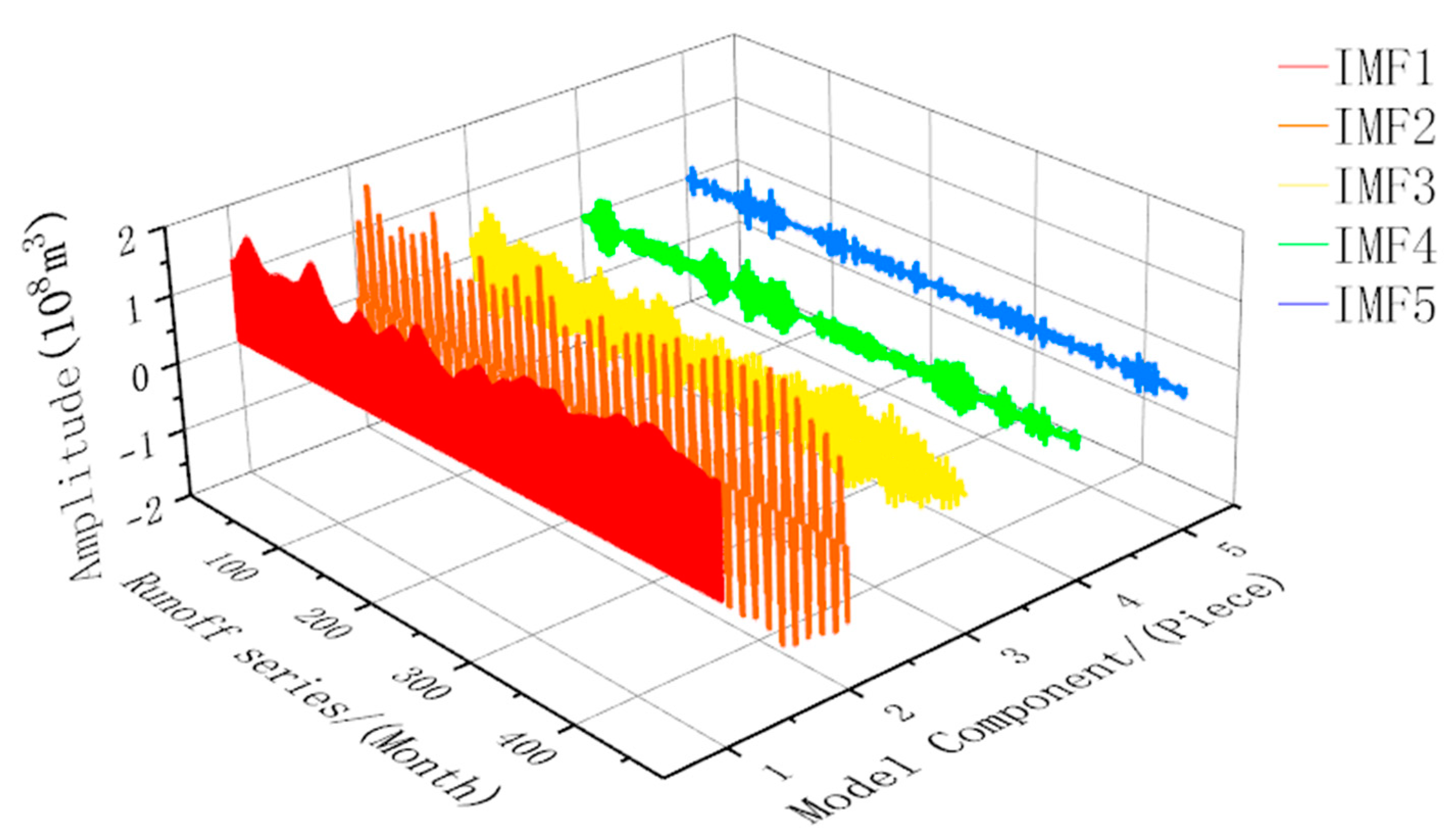
The above diagram shows that when K is five, the corresponding center frequency is relatively dispersed; when K is six, mode overlap occurs. In order to satisfy the orthogonality constraint and avoid spurious components as much as possible, the original runoff sequence is decomposed into five subsequences, and the two parameters γ and α of the model are set to 0 and 5000, respectively. The five obtained subsequences of monthly runoff are shown in the following figure (Figure 5).

3.2. Runoff Estimation

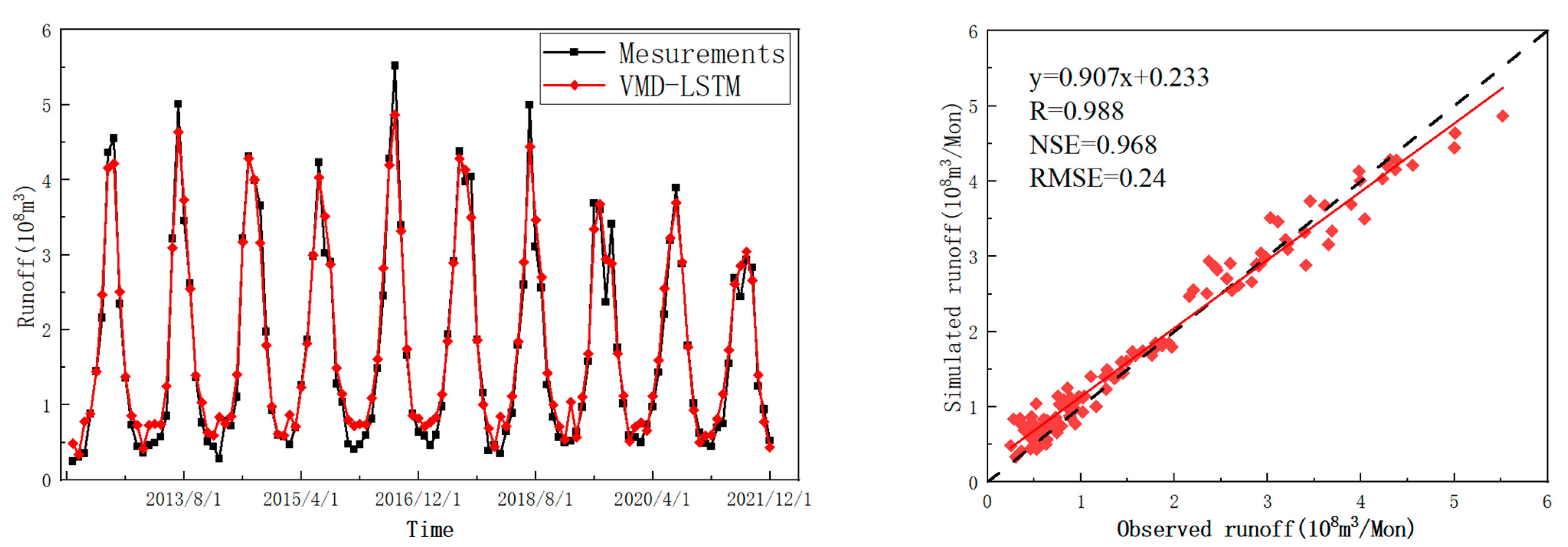
The VMD method is used to decompose the original runoff series into five runoff mode components. After determining the input lag time of each subsequence based on the MI method, the training set and test set are divided at a ratio of 3:1 and input into the LSTM deep learning network for simulation. After the completion of each sub-modal training, a reconstructed runoff series is obtained by inverse normalization and the cumulative addition of each prediction component. The final prediction effect of the VMD-LSTM model is shown in Figure 6. Figure 6 shows that the VMD-LSTM model constructed in this paper performs very well in predicting monthly runoff in the Yingluoxia Gorge area in the upper reaches of the Heihe River. The forecasts are accurate in both the flood and dry seasons, and the runoff series predictions and measured values are well-matched. The proposed model achieves good prediction accuracy in this area, which indicates that the LSTM deep learning method based on VMD can be feasibly used for monthly runoff simulation in the study area.

3.3. Comparing Single and Hybrid Forecasting Models

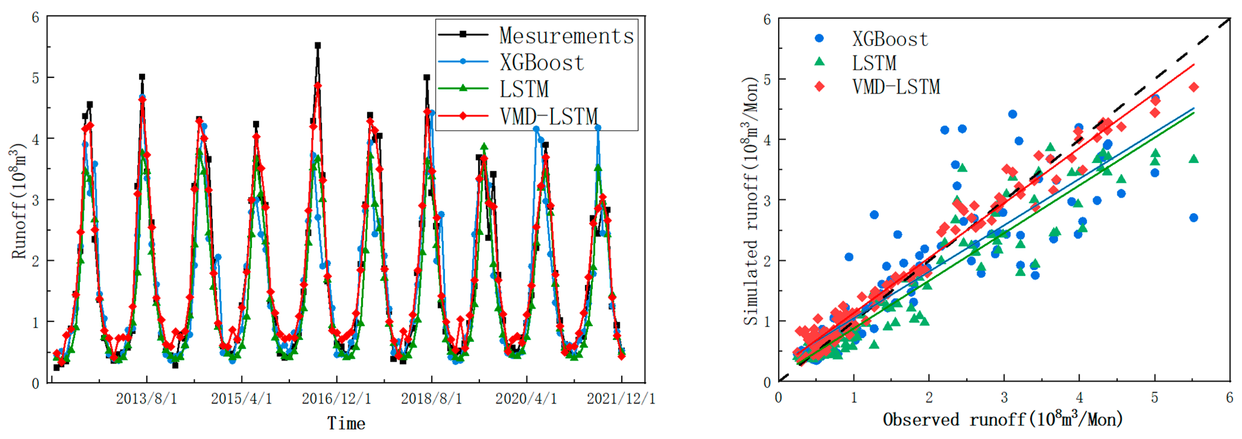
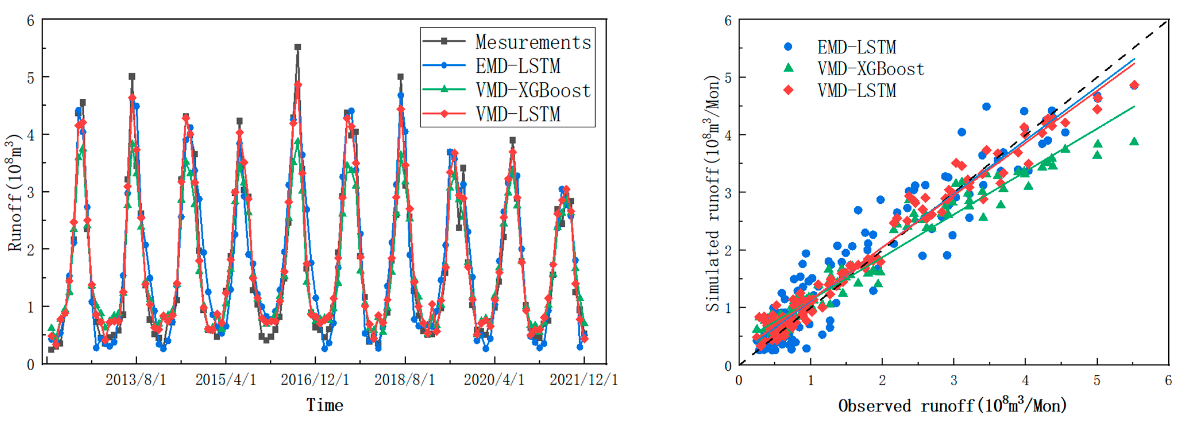
To further investigate the excellent performance of the model in monthly runoff prediction in the upper reaches of the Heihe River Basin, the VMD-LSTM model is compared with different single and combined models. The maximum number of iterations n_estimator, the learning rate, and the maximum tree depth in the XGBoost model are set to 65, 0.6, and 7, respectively. EMD is used to decompose the original runoff series into six natural modes and a residual series. Figure 7 and Figure 8 show a comparison between the constructed model and the single and combined models, respectively.
As shown in Table 3, compared with a naive LSTM model, a naive XGBoost, the EMD-LSTM, and the VMD-XGBoost hybrid models, the VMD-LSTM model performs better. The correlation coefficient, RMSE, and NSE values of the proposed model are the best of all the models. An important index for evaluating the results of hydrological sequence forecasting, the NSE reaches more than 0.96, which represents a significant improvement compared with a naive LSTM. At the same time, compared with the naive model, the hybrid model shows much higher R and NSE values and a much lower RMSE. This also demonstrates the efficiency of the hybrid model.
Figure 7 shows a comparison between the VMD-LSTM model and single models in terms of the prediction and fitting effects. Table 3 and Figure 7 show that the constructed VMD-LSTM model displays obvious advantages in the prediction of peak runoff values. The predictions of the model are basically consistent with the actual runoff sequence. The R and NSE values reach 0.988 and 0.968, respectively, and the RMSE is 0.24. However, the prediction results of the single models display a large deviation from the actual values. The correlation coefficient and NSE of the LSTM model are 3.7% and 11.9% lower than those of the VMD-LSTM model, respectively, and the RMSE is 0.282 higher. The non-stationarity of the time series leads to this phenomenon. Due to the complex change trend of runoff data, a single model cannot be well fitted. Moreover, the LSTM model is superior to the XGBoost model, mainly because of the LSTM’s structure, which preserves important information at each time step through the forget gate, thus improving the prediction accuracy. It is worth mentioning that there is an error in the prediction of each subsequence, and the reconstruction of the subsequence will amplify the prediction error of the entire model. This means that the proposed model performs poorly in the dry period. In general, however, the prediction accuracy of the hybrid model has improved.
Figure 8 shows a comparison between the VMD-LSTM model and other combined models based on the test set prediction results. Compared with the combined models based on different time–frequency decomposition methods, VMD-LSTM displays notable advantages, with high prediction accuracy and an optimal prediction effect. As shown in Table 3 and Figure 8, the low prediction accuracy of the EMD-LSTM combined model is mainly due to the fact that EMD is prone to mode aliasing issues and end effects, leading to inaccurate prediction results for each component. At the same time, the prediction error increases after mode reconstruction. This result verifies the superiority of VMD in the decomposition of non-stationary time series, and the hybrid prediction models with signal decomposition perform better than single models.
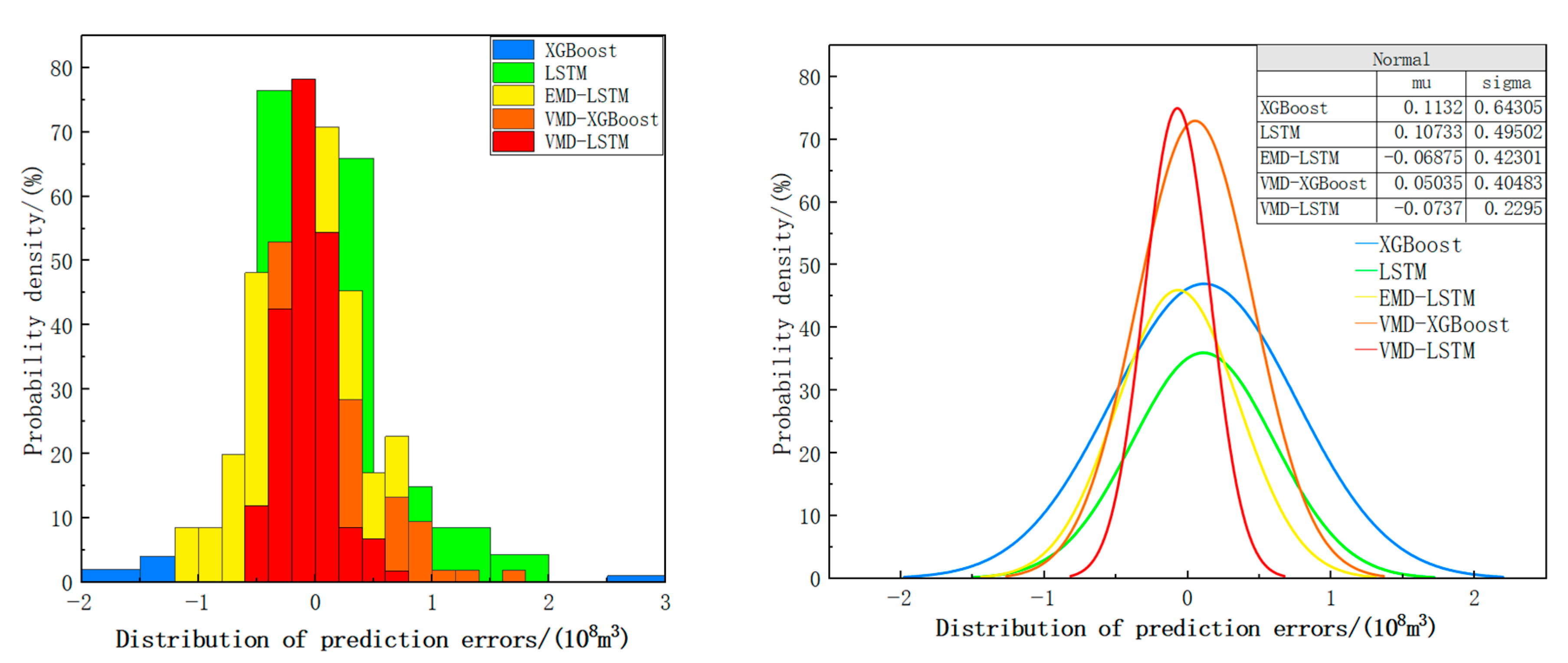
In Figure 9, the Gaussian frequency histogram and fitting distribution curve of each model error are shown. A Gaussian mixed-distribution test and statistical analysis were used to further analyze the distribution characteristics and simulation effects of each model. It can be seen that the VMD-LSTM model’s prediction error is concentrated around zero, while the error distributions of the other models are relatively wide, and the frequency of large errors is relatively high. The fluctuation in the prediction error of the proposed model is small, and the precision is high.

3.4. Runoff Interval Simulation

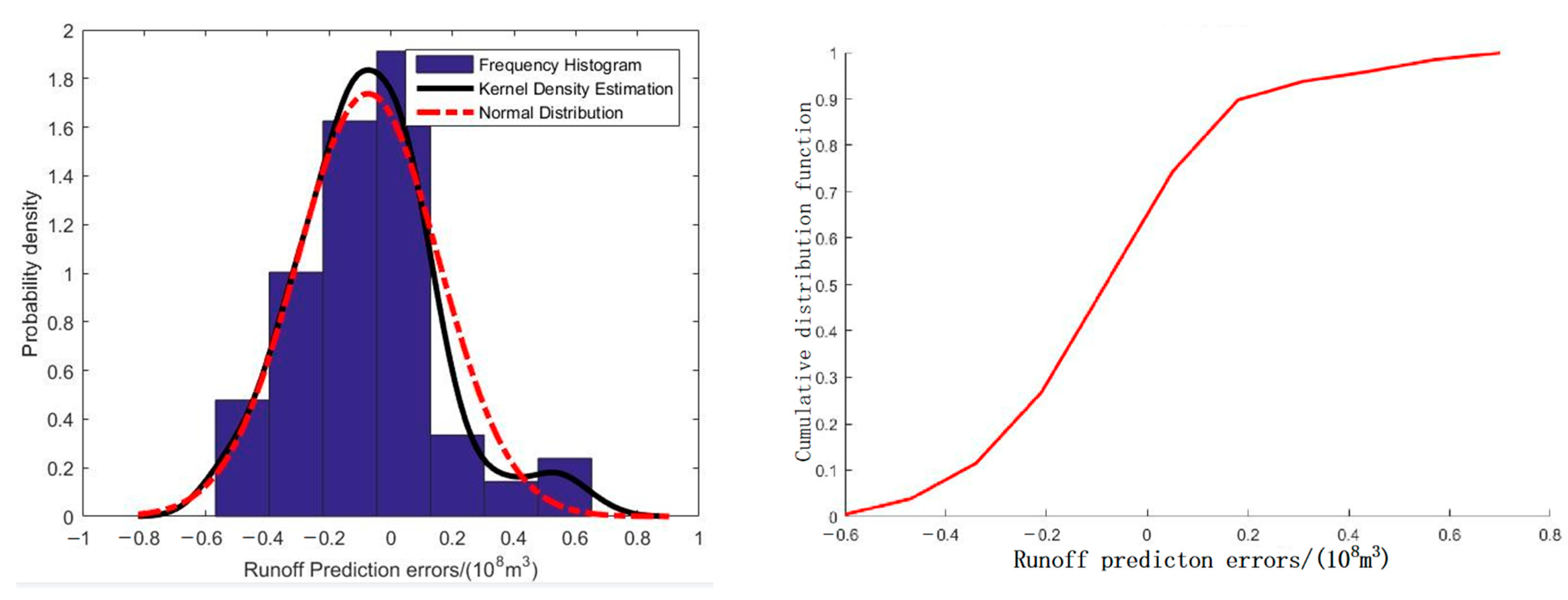
To evaluate the uncertainty of model predictions, we used the point prediction results to conduct an interval prediction analysis of the VMD-LSTM model based on the nonparametric KDE method. The error between the predicted and measured values is calculated, the statistical characteristics of the monthly runoff prediction error are analyzed, and the probability density function (PDF) of the error distribution is obtained based on the optimal window width by using the nonparametric KDE method with a Gaussian kernel function. Moreover, the cumulative distribution (CDF) of the error is obtained based on the PDF, as shown in Figure 10. Then, the predicted runoff error intervals at 95%, 90%, and 80% confidence levels are calculated, and the interval prediction results are evaluated based on the PICP and MPIW.
The CDF can be used to calculate the error intervals at 95%, 90%, and 80% confidence intervals; these values are [−0.4252, 0.3983], [−0.3863, 0.2189], and [−0.2645, 0.1148], respectively, as shown in Table 4. The prediction interval of the runoff series at each confidence level can be obtained by superimposing the error interval at each confidence level and the predicted values of the single-point runoff series. The distributions of the runoff intervals and measured values at three different confidence levels are shown in Figure 11.
For the predicted runoff series intervals and corresponding measured values at different confidence levels, the interval prediction results are evaluated by calculating the proportion of the measured values of the series in the prediction interval and the average interval width. Additionally, the interval prediction effects of different models are compared and analyzed. Table 5 shows that, for the same model, the PICP decreases as the confidence level decreases, and the MPIW also narrows. The prediction range of the VMD-LSTM model decreases from 0.8235 to 0.3793, and the prediction range becomes more detailed. Of the compared models, the mixed models display better coverage during the study period, and VMD-LSTM exhibits the highest coverage and the narrowest average width at each confidence interval, which verifies the excellent interval prediction performance of the model. Moreover, the prediction interval of the model obtained at a 90% confidence level encompasses the measured runoff values with large variations, and the coverage rate is high. The interval coverage of the model is high at 95% and 90% confidence levels, and the interval prediction effect is generally reliable. However, the interval coverage at the 80% confidence level is less than that at the other confidence levels, and the interval prediction result is not credible.

4. Discussion

Runoff prediction on a monthly scale is highly significant for water resource management and medium- and long-term dispatching and allocation. As an efficient neural network prediction model, the LSTM network has been widely used in hydrological prediction research. With the deepening of this research, a number of improved or combined models of LSTM have further surpassed the limits of its prediction performance and improved its prediction accuracy. Yuan, R. et al. [11] proved EEMD could improve the prediction performance of the LSTM model for runoff data. Zhang J. et al. [59] demonstrated the strong predictive performance of the fully connected LSTM when using time series data. Yuan X. et al. [18] optimized LSTM network parameters using an ant lion optimizer model to obtain better prediction results. Moreover, the amount of data is also an important factor affecting this deep learning model. For the single LSTM model assessed in this study, the final prediction results were not satisfactory because the model’s input data comprised only historical monthly runoff. As we all know, runoff is affected by many factors, and its changing trends become unstable. More important information can be obtained by decomposing the original runoff sequence. This provides data support for model fitting. In addition, the forecasting performance of VMD-based LSTM models is much better than that of EEMD-based LSTM models, because the phenomenon of mode aliasing occurs after EMD decomposition. In other words, the sub-signals of EMD have repeated information and hence chaotically represent the period, trend, and noise. In general, VMD can control the center frequency aliasing and noise level [29,62,63]. Thus, it is more appropriate for use in predicting runoff.
As an important part of the deep learning model, data input directly affects the final simulation results. In general, the selected input data are factors that are highly correlated with the predicted outcome. The mutual information method provides a more reasonable guarantee for model data input. This study determines the input lag time by measuring the relationship between the impact factor and the target, which greatly improves the quality of the data input. At the same time, the proposed model also provides a new way of thinking about runoff simulation in regions that lack data.
Interval prediction results can be used to quantify the uncertainty of monthly runoff, providing a reasonable range of monthly runoff fluctuations and comprehensive information for monthly runoff predictions [64,65]. In this paper, interval forecasting is carried out on the basis of point forecasting. The runoff fluctuations predicted by the proposed model are small in the interval prediction so that we can obtain more accurate and useful information from the prediction results. This provides a guarantee for reasonable water resource management and dispatching.
In summary, the framework constructed in this paper exhibits good performance in predicting the monthly runoff of the upper reaches of the Heihe River Basin. It shows that the time–frequency signal decomposition method can better deal with and analyze the signal information in non-stationary and nonlinear hydrological series. Moreover, the MI method and the LSTM network framework achieve accurate predictions by capturing this information. This study only uses historical runoff data to simulate future runoff. However, changes in runoff are significantly affected by human and meteorological factors. Further research should focus on how to effectively add such related factors to the model.

5. Conclusions

Using monthly runoff data from the Yingluoxia Hydrologic Station from 1982 to 2021, this study established an LSTM deep learning model based on VMD and an MI method to simulate the monthly runoff at Yingluoxia in the upper reaches of the Heihe River Basin in China. Based on a comparison of the point simulation prediction results of different single and combined models and an analysis of the interval prediction results of the VMD-LSTM model, the main conclusions can be summarized as follows:
(1)
The VMD method can effectively reduce the non-stationarity of hydrological time series, extract important hydrological feature information, and significantly improve the accuracy of runoff predictions. Compared with EMD, VMD can better control center frequency aliasing and noise levels.
(2)
Based on the MI method, the constructed VMD-LSTM model can effectively determine the input characteristics for deep learning. Overall, the proposed model performs well in runoff predictions. However, it should be noted that the accumulation of forecast errors for each subsequence affects the forecast result.
(3)
In interval prediction, the proposed model also yields satisfactory results. The prediction interval coverage and the simulation accuracy are high, and the average width is small. Interval prediction can be used to quantify the uncertainty of runoff predictions, estimate reasonable fluctuation ranges, and provide a certain reference for the establishment of hydrological prediction models and water resource management plans.
The continuous innovation in and improvement of deep learning methods will provide strong support for hydrological forecasting, significantly improve the accuracy of simulations, and provide scientific support for research on water resource utilization and hydrological prediction. The combination of time–frequency decomposition and deep learning when estimating runoff has yielded good results, providing a fast and cost-effective solution for runoff estimation in areas around the world where hydrological data are scarce. In addition, this method contributes to water resource management and scientific decision-making in the study region. Since the framework proposed in this study only relies on historical runoff data, it can be easily extended to runoff estimates from other hydrological stations. However, runoff is affected by many factors, so the accuracy of the prediction results for different time scales and regions has yet to be verified.

Author Contributions

Conceptualization, H.X., G.D. and H.W.; methodology, H.X., J.G. and G.D.; software, H.X. and H.W.; validation, H.W., J.G. and H.X.; formal analysis, H.W., G.D. and H.X.; investigation, H.X., G.D. and H.W.; resources, G.D.; data curation, G.D.; writing—original draft preparation, H.W.; writing—review and editing, H.W., H.X. and G.D.; visualization, H.W. and G.D.; funding acquisition, G.D. and H.X. All authors have read and agreed to the published version of the manuscript.

Funding

This research was funded by the National Natural Science Foundation of China, grant number 42061056.

Data Availability Statement

Monthly meteorological and hydrologic data were obtained from the Heihe River Bureau of the Yellow River Conservancy Commission (http://hrb.yrcc.gov.cn/, accessed on 22 March 2023).

Conflicts of Interest

The authors declare no conflict of interest.

References

  1. Wang, W.C.; Chau, K.W.; Cheng, C.T.; Qiu, L. A comparison of performance of several artificial intelligence methods for forecasting monthly discharge time series. J. Hydrol. 2009, 374, 294–306. [Google Scholar] [CrossRef]
  2. Zhang, Y.; Chiew, F.H.S.; Zhang, L.; Li, H. Use of Remotely Sensed Actual Evapotranspiration to Improve Rainfall-Runoff Modeling in Southeast Australia. J. Hydrometeorol. 2009, 10, 969–980. [Google Scholar] [CrossRef]
  3. Jiang, D.; Li, L.; Li, J. Runoff variation affected by precipitation change and human activity in Hailiutu River basin, China. Chin. J. Popul. Resour. Environ. 2021, 12, 116–122. [Google Scholar]
  4. Qiu, L.; Peng, D.; Xu, Z.; Liu, W. Identification of the impacts of climate changes and human activities on runoff in the upper and middle reaches of the Heihe River basin, China. J. Water Clim. Chang. 2016, 7, 251–262. [Google Scholar] [CrossRef]
  5. Qin, Y.; Sun, X.; Li, B.; Merz, B. A nonlinear hybrid model to assess the impacts of climate variability and human activities on runoff at different time scales. Stoch. Environ. Res. Risk Assess. 2021, 35, 1917–1929. [Google Scholar] [CrossRef]
  6. Li, C.; Zhu, L.; He, Z.; Gao, H.; Qu, X. Runoff Prediction Method Based on Adaptive Elman Neural Network. Water 2019, 11, 1113. [Google Scholar] [CrossRef]
  7. Young, C.-C.; Liu, W.-C.; Wu, M.-C. A physically based and machine learning hybrid approach for accurate rainfall-runoff modeling during extreme typhoon events. Appl. Soft. Comput. 2017, 53, 205–216. [Google Scholar] [CrossRef]
  8. Liu, Y.; Zhang, T.; Kang, A.; Li, J.; Lei, X. Research on Runoff Simulations Using Deep-Learning Methods. Sustainability 2021, 13, 1336. [Google Scholar] [CrossRef]
  9. Pathiraja, S.; Moradkhani, H.; Marshall, L.; Sharma, A.; Geenens, G. Data-driven model uncertainty estimation in hydrologic data assimilation. Water Resour. Res. 2018, 54, 1252–1280. [Google Scholar] [CrossRef]
  10. Ghaith, M.; Siam, A.; Li, Z.; El-Dakhakhni, W. Hybrid hydrological data-driven approach for daily streamflow forecasting. J. Hydrol. Eng. 2020, 25, 04019063. [Google Scholar] [CrossRef]
  11. Yuan, R.; Cai, S.; Liao, W.; Lei, X.; Xu, Y. Daily Runoff Forecasting Using Ensemble Empirical Mode Decomposition and Long Short-Term Memory. Front. Earth Sci. 2021, 9, 621780. [Google Scholar] [CrossRef]
  12. Ghanbarzadeh, M.; Aminghafari, M. A novel wavelet artificial neural networks method to predict non-stationary time series. Commun. Stat. Theory Methods 2020, 49, 864–878. [Google Scholar] [CrossRef]
  13. Wang, H.; Wu, X.; Gholinia, F. Forecasting hydropower generation by GFDL-CM3 climate model and hybrid hydrological-Elman neural network model based on Improved Sparrow Search Algorithm (ISSA). Concurr. Comput. Pract. Exp. 2021, 33, e6476. [Google Scholar] [CrossRef]
  14. Kelleher, J.D. Deep Learning; MIT Press: Cambridge, MA, USA, 2019. [Google Scholar]
  15. Li, Z.; Kang, L.; Zhou, L.; Zhu, M. Deep learning framework with time series analysis methods for runoff prediction. Water 2021, 13, 575. [Google Scholar] [CrossRef]
  16. Sherstinsky, A. Fundamentals of recurrent neural network (RNN) and long short-term memory (LSTM) network. Phys. D Nonlinear Phenom. 2020, 404, 132306. [Google Scholar] [CrossRef]
  17. Kratzert, F.; Klotz, D.; Brenner, C.; Schulz, K.; Herrnegger, M. Rainfall–runoff modelling using long short-term memory (LSTM) networks. Hydrol. Earth Syst. Sci. 2018, 22, 6005–6022. [Google Scholar] [CrossRef]
  18. Yuan, X.; Chen, C.; Lei, X.; Yuan, Y.; Muhammad Adnan, R. Monthly runoff forecasting based on LSTM–ALO model. Stoch. Environ. Res. Risk Assess. 2018, 32, 2199–2212. [Google Scholar] [CrossRef]
  19. Li, W.; Kiaghadi, A.; Dawson, C. High temporal resolution rainfall–runoff modeling using long-short-term-memory (LSTM) networks. Neural Comput. Appl. 2021, 33, 1261–1278. [Google Scholar] [CrossRef]
  20. Xue, H.; Liu, J.; Dong, G.; Zhang, C.; Jia, D. Runoff Estimation in the Upper Reaches of the Heihe River Using an LSTM Model with Remote Sensing Data. Remote Sens. 2022, 14, 2488. [Google Scholar] [CrossRef]
  21. Seo, Y.; Kim, S.; Singh, V.P. Machine Learning Models Coupled with Variational Mode Decomposition: A New Approach for Modeling Daily Rainfall-Runoff. Atmosphere 2018, 9, 251. [Google Scholar] [CrossRef]
  22. Lu, J.; Li, A. Monthly Runoff Prediction Using Wavelet Transform and Fast Resource Optimization Network (Fron) Algorithm. J. Phys. Conf. Ser. 2019, 1302, 042005. [Google Scholar] [CrossRef]
  23. Ding, Z.; Zhang, J.; Xie, G. LS-SVM forecast model of precipitation and runoff based on EMD. In Proceedings of the Sixth International Conference on Natural Computation, Yantai, China, 10–12 August 2010. [Google Scholar]
  24. Feng, Z.-K.; Niu, W.-J.; Tang, Z.-Y.; Jiang, Z.-Q.; Xu, Y.; Liu, Y.; Zhang, H.-R. Monthly runoff time series prediction by variational mode decomposition and support vector machine based on quantum-behaved particle swarm optimization. J. Hydrol. 2020, 583, 124627. [Google Scholar] [CrossRef]
  25. Zhao, X.; Chen, X.; Yuan, X. Application of data-driven model based on empirical mode decomposition for runoff forecasting. Syst. Eng. 2014, 32, 150–154. [Google Scholar]
  26. Li, B.J.; Sun, G.L.; Liu, Y.; Wang, W.C.; Huang, X.D. Monthly Runoff Forecasting Using Variational Mode Decomposition Coupled with Gray Wolf Optimizer-Based Long Short-term Memory Neural Networks. Water Resour. Manag. 2022, 36, 2095–2115. [Google Scholar] [CrossRef]
  27. Muhammad, S.; Li, X.; Bashir, H.; Azam, M.I. A Hybrid Model for Runoff Prediction Using Variational Mode Decomposition and Artificial Neural Network. Water Resour. 2021, 48, 701–712. [Google Scholar] [CrossRef]
  28. Zhu, S.; Zhou, J.; Ye, L.; Meng, C. Streamflow estimation by support vector machine coupled with different methods of time series decomposition in the upper reaches of Yangtze River, China. Environ. Earth Sci. 2016, 75, 531.1–531.12. [Google Scholar] [CrossRef]
  29. Zuo, G.; Luo, J.; Wang, N.; Lian, Y.; He, X. Decomposition ensemble model based on variational mode decomposition and long short-term memory for streamflow forecasting. J. Hydrol. 2020, 585, 124776. [Google Scholar] [CrossRef]
  30. Kasiviswanathan, K.; Cibin, R.; Sudheer, K.; Chaubey, I. Constructing prediction interval for artificial neural network rainfall runoff models based on ensemble simulations. J. Hydrol. 2013, 499, 275–288. [Google Scholar] [CrossRef]
  31. Chen, X.; Lai, C.S.; Ng, W.W.Y.; Pan, K.; Zhong, C. A stochastic sensitivity-based multi-objective optimization method for short-term wind speed interval prediction. Int. J. Mach. Learn. Cybern. 2021, 12, 2579–2590. [Google Scholar] [CrossRef]
  32. Kiefer, M.; Heimel, M.; Breß, S.; Markl, V. Estimating join selectivities using bandwidth-optimized kernel density models. Proc. VLDB Endow. 2017, 10, 2085–2096. [Google Scholar] [CrossRef]
  33. Yang, X.; Xue, M.; Ning, K.; Maihemuti, M. Probability Interval Prediction of Wind Power Based on KDE Method With Rough Sets and Weighted Markov Chain. IEEE Access 2018, 6, 51556–51565. [Google Scholar] [CrossRef]
  34. Du, B.; Huang, S.; Guo, J.; Tang, H.; Wang, L.; Zhou, S. Interval forecasting for urban water demand using PSO optimized KDE distribution and LSTM neural networks. Appl. Soft Comput. 2022, 122, 108875. [Google Scholar] [CrossRef]
  35. Zhang, L.; Xie, L.; Han, Q.; Wang, Z.; Huang, C. Probability Density Forecasting of Wind Speed Based on Quantile Regression and Kernel Density Estimation. Energies 2020, 13, 6125. [Google Scholar] [CrossRef]
  36. Zhang, L.; Su, F.; Yang, D.; Hao, Z.; Tong, K. Discharge regime and simulation for the upstream of major rivers over Tibetan Plateau. J. Geophys. Res. D. Atmos. JGR 2013, 118, 118. [Google Scholar] [CrossRef]
  37. Cheng, G.D.; Xiao, H.L.; Xu, Z.M.; Li, J.X.; Lu, M.F. Water Issue and Its Countermeasure in the Inland River Basins of Northwest China—A Case Study in Heihe River Basin. J. Glaciol. Geocryol. 2006, 28, 8. [Google Scholar]
  38. Wang, J.; Meng, J.J. Characteristics and Tendencies of Annual Runoff Variations in the Heihe River Basin During the Past 60 years. Sci. Geogr. Sin. 2008, 28, 83–88. [Google Scholar]
  39. Wang, Y.; Yang, D.; Lei, H.; Yang, H. Impact of cryosphere hydrological processes on the river runoff in the upper reaches of Heihe River. J. Hydraul. Eng. 2015, 46, 1064–1071. [Google Scholar] [CrossRef]
  40. Chen, D.; Jin, G.; Zhang, Q.; Arowolo, A.O.; Li, Y. Water ecological function zoning in Heihe River Basin, Northwest China. Phys. Chem. Earth 2016, 96, 74–83. [Google Scholar] [CrossRef]
  41. Dragomiretskiy, K.; Zosso, D. Variational mode decomposition. IEEE Trans. Signal Process. 2013, 62, 531–544. [Google Scholar] [CrossRef]
  42. Zhou, M.; Hu, T.; Bian, K.; Lai, W.; Hu, F.; Hamrani, O.; Zhu, Z. Short-Term Electric Load Forecasting Based on Variational Mode Decomposition and Grey Wolf Optimization. Energies 2021, 14, 4890. [Google Scholar] [CrossRef]
  43. Naik, J.; Dash, S.; Dash, P.K.; Bisoi, R. Short term wind power forecasting using hybrid variational mode decomposition and multi-kernel regularized pseudo inverse neural network. Renew. Energy 2018, 118, 180–212. [Google Scholar] [CrossRef]
  44. Banik, A.; Behera, C.; Sarathkumar, T.V.; Goswami, A.K. Uncertain wind power forecasting using LSTM-based prediction interval. IET Renew. Power Gener. 2020, 14, 2657–2667. [Google Scholar] [CrossRef]
  45. Božić, M.; Stojanović, M.; Stajić, Z.; Floranović, N. Mutual Information-Based Inputs Selection for Electric Load Time Series Forecasting. Entropy 2013, 15, 926–942. [Google Scholar] [CrossRef]
  46. Lv, N.; Liang, X.; Chen, C.; Zhou, Y.; Wang, H. A Long Short-Term Memory Cyclic model With Mutual Information For Hydrology Forecasting: A Case Study in the Xixian Basin. Adv. Water Resour. 2020, 141, 103622. [Google Scholar] [CrossRef]
  47. Kraskov, A.; Stögbauer, H.; Grassberger, P. Estimating mutual information. Physical Rev. E 2004, 69, 066138. [Google Scholar] [CrossRef]
  48. Chen, J.; Wu, Z.; Zhang, J.A.; Li, F.A. Mutual information-based dropout: Learning deep relevant feature representation architectures. Neurocomputing 2019, 361, 173–184. [Google Scholar] [CrossRef]
  49. Li, G.; Zhao, X.; Fan, C.; Fang, X.; Li, F.; Wu, Y. Assessment of long short-term memory and its modifications for enhanced short-term building energy predictions—ScienceDirect. J. Build. Eng. 2021, 43, 103182. [Google Scholar] [CrossRef]
  50. Hochreiter, S.; Schmidhuber, J. Long Short-Term Memory. Neural Comput. 1997, 9, 1735–1780. [Google Scholar] [CrossRef]
  51. Xiang, Z.; Yan, J.; Demir, I. A rainfall-runoff model with LSTM-based sequence-to-sequence learning. Water Resour. Res. 2020, 56, e2019WR025326. [Google Scholar] [CrossRef]
  52. Xu, Y.; Hu, C.; Wu, Q.; Jian, S.; Li, Z.; Chen, Y.; Zhang, G.; Zhang, Z.; Wang, S. Research on particle swarm optimization in LSTM neural networks for rainfall-runoff simulation. J. Hydrol. 2022, 608, 127553. [Google Scholar] [CrossRef]
  53. Terrell, G.R.; Scott, D.W. Variable kernel density estimation. Ann. Stat. 1992, 20, 1236–1265. [Google Scholar] [CrossRef]
  54. Zhou, B.; Ma, X.; Luo, Y.; Yang, D. Wind power prediction based on LSTM networks and nonparametric kernel density estimation. IEEE Access 2019, 7, 165279–165292. [Google Scholar] [CrossRef]
  55. Pan, C.; Tan, J.; Feng, D. Prediction intervals estimation of solar generation based on gated recurrent unit and kernel density estimation. Neurocomputing 2021, 453, 552–562. [Google Scholar] [CrossRef]
  56. Jiang, Y.; Huang, G.; Yang, Q.; Yan, Z.; Zhang, C. A novel probabilistic wind speed prediction approach using real time refined variational model decomposition and conditional kernel density estimation. Energy Convers. Manag. 2019, 185, 758–773. [Google Scholar] [CrossRef]
  57. Peel, S.; Wilson, L.J. Modeling the distribution of precipitation forecasts from the Canadian ensemble prediction system using kernel density estimation. Weather. Forecast. 2008, 23, 575–595. [Google Scholar] [CrossRef]
  58. Bai, M.; Zhao, X.; Long, Z.; Liu, J.; Yu, D. Short-term probabilistic photovoltaic power forecast based on deep convolutional long short-term memory network and kernel density estimation. arXiv 2021, arXiv:2107.01343. [Google Scholar]
  59. Zhanga, J.; Yan, Z.; Zhanga, X.; Ming, Y.; Yangb, J. Developing a Long Short-Term Memory (LSTM) based model for predicting water table depth in agricultural areas. J. Hydrol. 2018, 561, 918–929. [Google Scholar] [CrossRef]
  60. Wang, X.; Wang, Y.; Yuan, P.; Wang, L.; Cheng, D. An adaptive daily runoff forecast model using VMD-LSTM-PSO hybrid approach. Hydrol. Sci. J. 2021, 66, 1488–1502. [Google Scholar] [CrossRef]
  61. Yang, H.; Chao, J.; Shi, K.; Liu, S. Fault Information Extraction Method for Rolling Bearings Based on VMD Parameter Estimation. Bearing 2016, 10, 49–52. [Google Scholar]
  62. Chen, S.; Ren, M.; Sun, W. Combining two-stage decomposition based machine learning methods for annual runoff forecasting. J. Hydrol. 2021, 603, 126945. [Google Scholar] [CrossRef]
  63. Niu, H.; Xu, K.; Wang, W. A hybrid stock price index forecasting model based on variational mode decomposition and LSTM network. Appl. Intell. 2020, 50, 4296–4309. [Google Scholar] [CrossRef]
  64. Zhang, K.; Ma, P.; Cui, Z.; Xing, T.; Qi, C.; Ning, G.; Amp, E. Ultra-short term wind power output interval forecast model based on ASD-KDE algorithm. Ningxia Electr. Power 2018, 2018, 8. [Google Scholar]
  65. Zhao, M.; Zhang, Y.; Hu, T.; Wang, P. Interval Prediction Method for Solar Radiation Based on Kernel Density Estimation and Machine Learning. Complexity 2022, 2022, 7495651. [Google Scholar] [CrossRef]
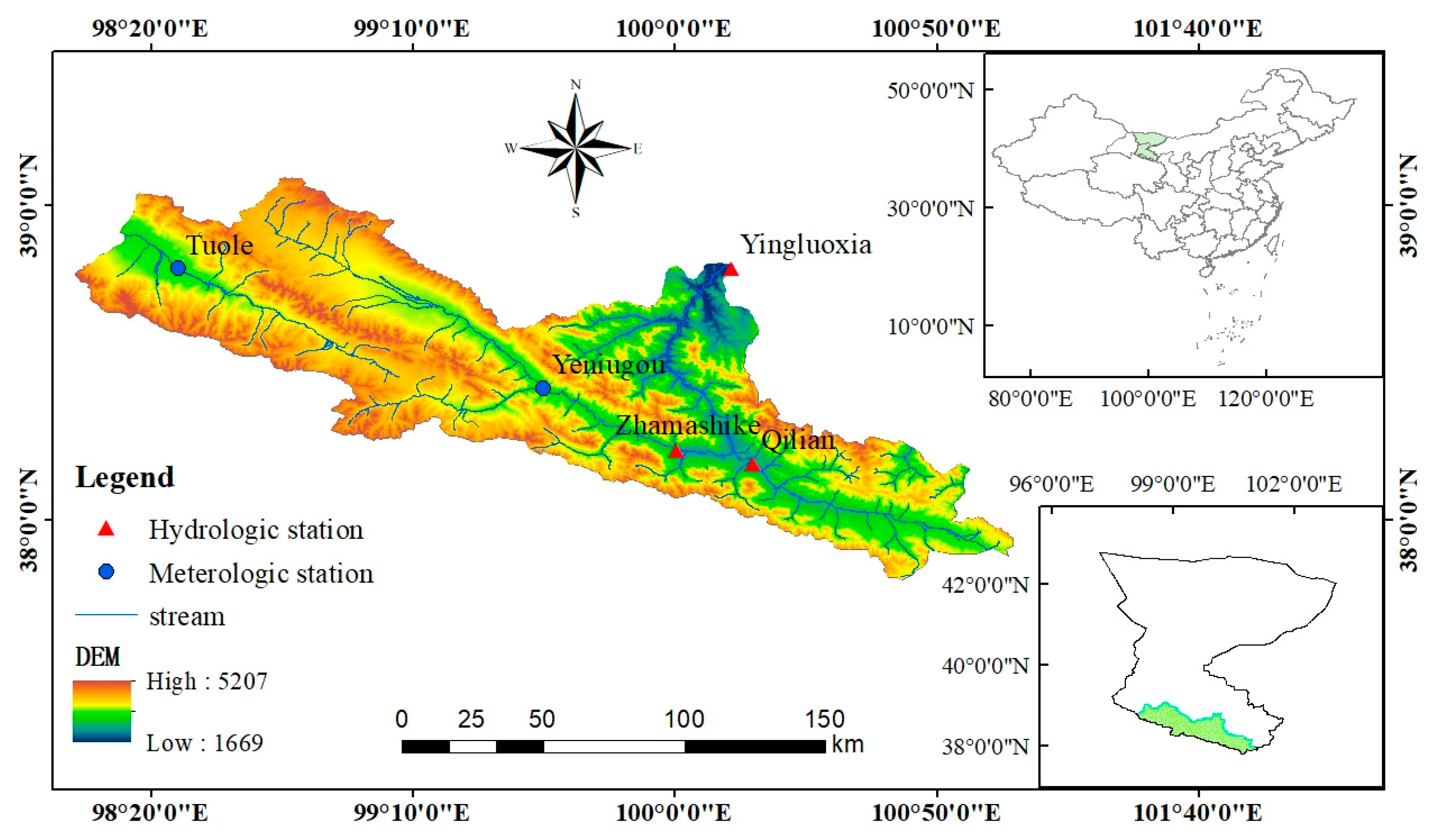
Figure 1. Upper reaches of the Heihe River Basin. The red triangles correspond to three hydrologic stations. The blue circles represent the meteorological stations in the upper Heihe River Basin.
Sustainability 15 07819 g001
Figure 2. The basic structure of an LSTM cell. The black arrows indicate the directions of the data flows. The gray rectangles indicate activation functions. The orange symbols represent calculation steps.
Sustainability 15 07819 g002
Figure 3. Monthly runoff forecasting process based on VMD-LSTM. The dashed black box denotes the runoff simulation steps in the LSTM model.
Sustainability 15 07819 g003
Figure 4. The center frequency of the final modes after decomposition when the number of components is 5 and 6.
Sustainability 15 07819 g004
Figure 5. Decomposition results for all modes. The red, orange, yellow, green, and blue line segments represent the five modes after the completion of VMD.
Sustainability 15 07819 g005
Figure 6. Runoff predictions of the VMD-LSTM model. In the (left) half, the black and red lines represent the observed and estimated runoff values, respectively. On the (right) side, the red line indicates the linear regression trendline for the observed and simulated runoff values. The black dotted line is a 1:1 line.
Sustainability 15 07819 g006
Figure 7. Comparison with a single model. The black dotted line is a 1:1 line.
Sustainability 15 07819 g007
Figure 8. Comparison of the proposed model and hybrid models. The black dotted line is a 1:1 line.
Sustainability 15 07819 g008
Figure 9. Error distributions of different models; (left) is the Gaussian frequency histogram, and (right) shows the fitting distribution curves.
Sustainability 15 07819 g009
Figure 10. Error distribution for runoff estimation; (left) is the probability density function (PDF), and (right) is the cumulative distribution function (CDF).
Sustainability 15 07819 g010
Figure 11. Estimation of runoff intervals at different confidence levels: (a) 95% confidence interval; (b) 90% confidence interval; and (c) 80% confidence interval.
Sustainability 15 07819 g011
Table 1. Previous studies of runoff prediction methods.
CategorySub-CategoryAdvantagesLimitations
Process-driven modelsConceptual models (tank model,
storage function)
Relatively easy to calculate; can express various runoff patternsParameters lack physical meaning
Physical models (distributed models)Runoff process is expressed in detail; reflects topography and rainfall distributionRequired data are difficult to obtain;
model building is time consuming
Data-driven modelsTime-series models (AR, ARMA, ARIMA, etc.)Models are easily constructed Cannot simulate complex and nonlinear runoff
Machine learning (linear regression,
SVM, ANN, RNN, etc.)
Strong ability to deal with nonlinear problemsCalculation process is “black box”; requires a considerable amount of data
Table 2. Statistics for monthly runoff data.
Runoff SampleLength/MonthsMean/108 m3Standard Deviation/108 m3Coefficient of VariationSkewness
Total4801.491.2560.8421.31
Training period3601.4171.2160.8580.92
Verification period1201.7151.3510.7881.2
Table 3. Runoff estimation results of different models.
ModelRRMSENSE
XGBoost0.8790.650.766
LSTM0.9510.5220.849
EMD-LSTM0.950.4270.899
VMD-XGBoost0.9790.4060.909
VMD-LSTM0.9880.240.968
Table 4. Estimation error intervals at different confidence levels.
Confidence Interval/%Estimation Error Interval
95[−0.4252, 0.3983]
90[−0.3863, 0.2189]
80[−0.2645, 0.1148]
Table 5. Estimation interval evaluation of models at different confidence levels.
ModelConfidence Interval/%Number of Measured Values within the IntervalPICPMPIW
XGBoost95980.81671.5615
90860.71671.3678
80720.61.0125
LSTM95960.81.4012
90890.74171.2924
80740.61670.9085
EMD-LSTM951060.88331.1137
90970.80830.9124
80860.71660.6114
VMD-XGBoost951060.88331.0685
90990.8250.8861
80870.7250.5124
VMD-LSTM951160.96670.8235
901090.90830.6052
80920.76670.3793
Disclaimer/Publisher’s Note: The statements, opinions and data contained in all publications are solely those of the individual author(s) and contributor(s) and not of MDPI and/or the editor(s). MDPI and/or the editor(s) disclaim responsibility for any injury to people or property resulting from any ideas, methods, instructions or products referred to in the content.