
The Green Lung: National Parks and Air Quality in Italian Municipalities
by
 , and
, and
Leonardo Becchetti
1,*,
Gabriele Beccari
1,2,
Gianluigi Conzo
1,
Davide De Santis
3 ,
,
Pierluigi Conzo
4,5 and
Francesco Salustri
6,7 1
Department of Economics and Finance, University of Rome Tor Vergata, 00133 Rome, Italy
2
Faculty of Political and Social Sciences, Scuola Normale Superiore, 56126 Pisa, Italy
3
Department of Civil Engineering and Computer Science Engineering, University of Rome Tor Vergata, 00133 Rome, Italy
4
Department of Economics and Statistics “Cognetti de Martiis”, University of Turin, 10153 Torino, Italy
5
Collegio Carlo Alberto, University of Turin, 10122 Torino, Italy
6
Department of Economics, Roma Tre University, 00145 Rome, Italy
7
Institute for Global Health, University College London, London WC1N 1DP, UK
*
Author to whom correspondence should be addressed.
Sustainability 2023, 15(10), 7802; https://doi.org/10.3390/su15107802
Submission received: 10 February 2023
/
Revised: 23 April 2023
/
Accepted: 26 April 2023
/
Published: 10 May 2023
(This article belongs to the Special Issue Air Pollution Prevention and Environmental Management)
Abstract
:In Italy, 25 percent of the 7903 municipalities include protected areas, while 6.4 percent—which we define as park municipalities—are national parks. Using data from the Copernicus programme databases, we investigated the relationship between park municipalities and the air quality, and we found that the air pollution levels in these areas were much lower than in the rest of the municipalities for the period 2017–2020. The gross difference ranged from 25 to 30 percent lower levels of particulate matter (as measured in terms of both PM10 and PM2.5), and three times lower levels of nitrogen dioxide. In our multivariate econometric analysis, we found that part of this difference depends on the lower population density and manufacturing activity in municipalities with national parks. Furthermore, we showed that park municipalities: (i) had progressively reduced levels of particulate matter during the period 2017–2020, and (ii) had a “green lung” function, since in non-park municipalities’ air pollution levels increased with the distance from national parks. Based on empirical evidence on the impact of the main air pollutants on mortality documented in the literature, we calculated that living in park municipalities reduces mortality rates by around 10 percent.
1. Introduction
The value of natural capital has been extensively investigated in the economic literature. Ref. [1] estimated the value of ecosystem services for the entire biosphere, most of which are determined by non-directly marketable activities, such as clean air, soil quality and fertility, and uncontaminated water. The authors find that the value is around twice the value of the world gross domestic product. On the role of natural capital, Ref. [2] emphasised that preservation of natural capital is the often-neglected essential pre-condition to achieve sustainable development. More recently, Ref. [3] showed that natural capital has a significant impact on life satisfaction among countries at a similar stage of human development.
The quality of natural capital is crucial to achieve the ecological transition goals set by international institutions and, in particular, the Sustainable Development Goals 3 (Good Health and Wellbeing), 6 (Clean Water and Sanitation), 7 (Sustainable Cities and Communities), 12 (Responsible Consumption and Production), 13 (Climate Action), 14 (Life below Water), and 15 (Life on Land). In this direction, the “do not cause significant harm” principle proposed by the European Commission states that national recovery and resilience plans should not harm the following six environmental objectives: adaptation to climate change, mitigation of climate change, sustainable use and protection of water and maritime resources, circular economy, prevention and control, and protection and restoration of biodiversity and ecosystems (Regulation (EU) 2020/852 of the European Parliament and of the Council of 18 June 2020 on the establishment of a framework to facilitate sustainable investment, and amending Regulation (EU) 2019/2088 (Text with EEA relevance): https://eur-lex.europa.eu/eli/reg/2020/852/oj, accessed on 27 April 2023).
In our paper, we studied to what extent natural parks in Italy contribute, via their high natural capital stock, to these goals, and we focused on air quality, as measured by particulate matter (both PM10 and PM2.5), as our measure of ambient air pollution. The Italian context is more than suitable for investigating this issue as more than 25 percent of its municipalities contain protected areas, such as national or regional parks, or marine-protected areas, and 6.4 percent of them have part of their areas in national parks.
According to the Italian law No. 394, 6 December 1991, a national park is defined as a land, river, lake, or marine area containing one or more ecosystems that are intact or partially altered by human intervention. In this national park, the physical, geological, geomorphological, and biological formations that contribute to the aforementioned ecosystem must be of international or national interest for their naturalistic, scientific, aesthetic, cultural, educational, and recreational values. Due to such an interest, the government regularly provides interventions for prevention and maintenance in the public interest of current and future generations. In addition, in these areas, the government requires the development of socioeconomic activities that are compatible with the conservation of biodiversity, and support local citizens’ participation, local economic development, and cultural and civil growth aimed at preserving territorial identities. National parks in Italy are founded from public sources and are managed by national and regional administrations.
In this study, we exploited this Italian peculiarity to evaluate the effects of park municipalities (i.e., municipalities partially or totally located within natural parks) on air quality and health. More specifically, we tested the following three research hypotheses. First, we analysed whether park municipalities exhibited significantly lower levels of air pollution than non-park municipalities in the period 2017–2020. Second, we examined the difference between air quality in park and non-park municipalities, to see if this has grown over time. Third, we tried to check the robustness of our previous results by looking at whether national parks generate positive environmental externalities outside their borders; that is, whether the level of pollution in non-park municipalities increases as the distance from the closest national park increases. Finally, we computed the expected impact of the difference in air quality between park and non-park municipalities on mortality rates.
Our empirical analysis contributes to different strands of the literature on natural parks, environmental measures, and health outcomes. Several studies document that people living in national parks enjoy better health conditions. This is due to the fact that national parks provide opportunities to increase physical activity levels, thus reducing obesity, and they also generate lower levels of distress, improving mental health [4,5,6,7,8,9]. With a focus on air quality, our paper also contributes to a long-standing literature that analyses the detrimental effect of poor air quality on a number of health outcomes. For example, Ref. [10] find that the reduction of nitrogen dioxide (NO2), sulphur dioxide (SO2), and PM10 emissions has a statistically significant and positive impact on health. Based on the estimated effect of pollution on health, Ref. [11] showed that a clear decision can be made on the acceptable number of statistical deaths due to pollution. In the same direction, Ref. [12] reviewed a large number of studies testing the correlation between long-term exposure to particulate matter and mortality. In a recent work, Ref. [13] analysed the effect of a reduction of PM2.5, ozone (O3), and NO2 among Medicare beneficiaries in Massachusetts, for the period 2000–2012. The authors found that a 1 μg/m3 increase in long- and short-term PM2.5 exposure is associated with 35.4 and 3.04 excess deaths per 10 million person-days, respectively, each 1-part per billion (ppb) increase in long- and short-term O3 exposure is associated with 2.35 and 2.41 excess deaths, respectively, and each 1 ppb increase in long- and short-term NO2 exposure is associated with 3.24 and 5.60 excess deaths, respectively. Similarly, Ref. [14] performed a spatial analysis to test positive associations of PM2.5, O3, and NO2 with mortality, using individualised exposure assessments for a sample in California. In Tehran, Iran, Ref. [15] investigated all-cause, non-accidental daily mortality and its association with fine PM2.5, NO2, and the Air Quality Index (AQI) from March 2011 to March 2014. This research shows that the relative risks for all seasons, both sexes, and all ages at lag 0 for PM2.5, NO2, and AQI were 1.004, 1.003, and 1.004, respectively, per interquartile range increment (18.8 μg/m3 for PM2.5, 12.6 ppb for NO2, and 31.5 for AQI). More specifically, for respiratory diseases, several studies tested whether the number of respiratory diseases in children and the elderly increases due to higher air pollution concentrations [16,17,18]. In the same direction, focusing on people of all ages, Ref. [19] examined the associations between the daily variations of air pollutants and health, finding a positive and statistically significant nexus between particulate matter and NO2, on the one hand, and hospital admissions for respiratory diseases on the other. They found that, for an increase of 10 μg/m3 in concentrations of the pollutants, the highest association of each pollutant with total hospital admissions was observed with PM2.5 at lag 4, NO2 at lag 4, and PM10 at lag 0. Similarly, Ref. [13] found positive associations between short-term exposure to PM2.5 and the risk of hospital admission. The authors showed that a 1 µg/m3 increase in short-term PM2.5 is associated with an annual increase of 2050 hospital admissions, 12,216 days in hospital, USD 31 m in inpatient and post-acute care costs, and USD 2.5 bn in the value of statistical life. For diseases with a previously known association, a 1 µg/m3 increase in short-term exposure to PM2.5 is associated with an annual increase of 3642 hospital admissions, 20,098 days in hospital, USD 69 m in inpatient and post-acute care costs, and USD 4.1 bn in the value of statistical life. Other research did not look at health effects directly, but analysed how sustainable tourism and mobility can increase in protected areas [20,21]. This robust evidence gathered in different periods and places around the world documents a positive association between air pollution and a number of health outcomes.
Our research originally contributed to this literature by showing how people living in municipalities located in national or regional parks or marine-protected areas enjoy significantly higher air quality, bridging a gap in the literature. To our knowledge, the link between air pollution and national parks has been addressed by very few scholars, whose research mainly focuses on the main factors that can reduce park natural capital, including air pollution, and therefore does not directly look at their positive effect [22,23]. On the link between air pollution and health, our research focuses on a different contribution of parks to health, since we analysed how a cleaner environment leads to lower levels of air pollution, which ultimately generates a health improvement and thereby translates into a reduction in mortality. More specifically, the impact of park municipalities on air pollution was computed with a multivariate analysis, calculating the effect of natural parks after controlling for all relevant measurable factors at the municipality level (population, employment, and meteorological variables, such as wind, rain, and radiation), and for regional, month, and day-of-the-week effects. The impact of park municipalities on health was calculated by computing the average point estimate of the estimated effect of a given pollutant on the mortality rate from different empirical contributions in the literature and applying this average to the effect of the park municipality.
We performed our econometric analysis using a dataset that collected information for all Italian municipalities in the period 2017–2020. This allowed us to control for several concurring factors, such as the economic and demographic characteristics of the municipality. We showed that air pollution grows for non-park municipalities in the distance from national parks. We calculated the gross and net effect of the park municipalities on air pollution levels. Then, based on previous meta-analyses of the effects of air pollution on health, we calculated the combined health effect of living in park municipalities on mortality rates. Our empirical findings showed that people living in park municipalities enjoy significantly higher air quality in terms of reduced daily concentrations of PM2.5, PM10, and NO2. This effect is only partially explained by the lower population density and manufacturing activity. We also showed that the benefit of the park municipality has grown over the period of our analysis and that parks act as “green lungs”, creating positive externalities in terms of air quality that are inversely proportional to their distance. In general, we estimated that these factors reduce mortality rates by 10 percent for people living in park municipalities.
2. Data Description
Our research focuses on the 7903 municipalities that constituted the Italian local administrative division back in 2020. Around 26.51 percent (2074) of the municipalities in our sample included protected areas, and 6.4 percent (501)—which we define as park municipalities—included national parks.
To perform our empirical analysis, we used Python to gather climatic and air quality variables from the Copernicus programme databases. Copernicus (https://www.copernicus.eu/en, accessed on 30 November 2022) is a European Earth Observation programme established in 2014 to be the follow-up to the past GMES initiative. Its importance is growing, and it is becoming dominant as an official source of data for measuring climate change and environmental sustainability. For further details on the characteristics of the climate dataset considered for this study, see [24], and https://climate.copernicus.eu/sites/default/files/repository/Events/ICR5/Posters/07_S1_MunozSabater.pdf (accessed on 1 March 2023). We relied on the Copernicus Atmospheric Monitoring Service (CAMS) and the Copernicus Climate Change Monitoring Service (C3S).
CAMS provides continuous data and information on atmospheric composition, and its service aims at assessing air pollutant effects and reducing toxic elements in the air that we breathe at the surface level. Among the databases provided by CAMS, we used the “European Air Quality Forecasts” dataset, that gathers information on the following six pollutants: PM2.5, PM10, NO2, SO2, O3, and carbon monoxide (CO), at seven height levels and at hourly steps. Data are the result of a combination of nine regional European air quality production systems and a combination with observations registered by the European Environment Agency (EEA). The regional air quality production system models are: CHIMERE, DEHM, EMEP, EURAD-IM, GEM-AQ, LOTOS-EUROS, MATCH, MOCAGE, and SILAM. The blend usage of these systems is called the ENSEMBLE median, values of which correspond to the median of all the different systems’ figures. The latter data were used for our analysis.
C3S produces data on human-made pollutants and makes performing evaluations as well as predictions on their effects on the environment possible. Among the data provided by C3S, we used the “ERA5-Land” dataset, that consists of climate variables obtained from a combination of surface-level observations registered by ground sensors and data provided by the H-TESSEL land surface model. From this database, we extracted data on wind, air temperature, total precipitation, and solar radiation. We performed the following adjustments: (i) from wind variables (eastward and northward wind components), we derived the module of the resulting vector, (ii) air temperature, originally measured in Kelvin, was translated into Celsius, (iii) total precipitation, originally measured in metres, was transformed into millimetres, and (iv) solar radiation was transformed from Joule to Watt per square metre, by dividing by 86,400 s to obtain the corresponding amount of daily radiation.
All climatic and air quality variables, provided with a spatial coverage of 0.1 × 0.1 long./lat. degree, were later processed and combined to analyse the information at the municipal level, the smallest possible administrative unit. To work with daily means, we averaged the values available at 8:00, 12:00, 20:00, and 24:00 for each day.
The Copernicus databases use a grid geographically covering the entire peninsula, but do not always guarantee that each and every municipality is associated with at least one observation laying within their territory. In regions with a high concentration of small and sometimes very small towns, it could occur that some of them to fall out of the net. To solve this problem, we used the closest distance approach by calculating every municipality’s centroid and attaching to it the Copernicus point with the minimum Euclidean distance. The average minimum distance recorded was less than 4 km, with a few outliers that did not affect the accuracy of our analysis.
Copernicus data estimate the amounts of pollutants at the breathing height with homogeneous spatial distribution and availability in time, without intervals or interruptions. This is important, especially when it comes to the object of our research (impact of parks on air quality over time). This is because air quality ground control units in fixed locations are not homogeneously distributed in space, across regions, and specifically, in the areas of our particular interest (national parks), and they can be subject to stopping for maintenance. Among the many research papers using CAMS data for these reasons, see [25,26,27].
Moreover, we considered the forecast dataset provided by the CAMS model as they are available with a higher spatial resolution with respect to other categories of the CAMS dataset, such as the “reanalysis” one. At the same time, we checked for a random subset of data that the difference in terms of absolute values of the pollutant concentration between forecast and reanalysis datasets was small, and that it did not impact the robustness of the analysis and the outcome of the work.
3. Descriptive and Econometric Empirical Findings
Figure 1a–f show the distribution of the six observed air pollutants observed in Italian municipalities between 1 January 2017 and 31 May 2020. Table 1 shows a full and detailed list of all variables used in this analysis, including the six pollutants. They show that, as is well-known, PM2.5, PM10, CO, and NO2 concentrations in the Po Valley in north Italy are extremely high as a result of anthropogenic factors and geomorphological characteristics. This is because, in addition to the high population density, commuter flows, and industrial activity, the orographic structure of the valley surrounded by high mountains makes the air more stagnant. Our maps show that the areas around Rome and Naples, respectively, the first and third largest city in Italy by population size, also register high concentrations of PM2.5, PM10, and NO2 concentrations, most likely due to their large population size and density. PM10 and SO2 concentrations are also high in Sicily, south Italy, due to atmospheric conditions and perturbations from the Sahara [28]. Note that in our sample period, the daily average of PM2.5 (that is, 12.44 µg/m3) was above the yearly average threshold advised by the World Health Organisation (WHO) for air quality (that is, 10 µg/m3) (see: https://www.who.int/news/item/02-05-2018-9-out-of-10-people-worldwide-breathe-polluted-air-but-more-countries-are-taking-action, accessed on 9 February 2023), with higher values in Po Valley, Rome, and Naples (see: https://www.euronews.com/2020/11/10/air-pollution-italy-persistently-broke-eu-clean-air-laws-rules-the-european-court-of-justi, accessed on 9 February 2023). The high levels of PM2.5 and PM10 in Italy represent an issue for Europe. On 10 November 2020, the European Court of Justice declared that Italy has “persistently and systematically” breached the European Union against small-particle air pollution, in a ruling supporting the legal action by Brussels against Rome.
In Figure 2, we show how national parks are distributed throughout the country, and in Table 2 we show descriptive differences in pollutant levels between park and non-park, with 95 percent confidence intervals. We observed that the PM concentration was one-third lower in park municipalities for PM2.5 and one-fourth lower for PM10. In both cases, we observed a difference of approximately 4 µg/m3 (8.71 µg/m3 vs. 12.82 µg/m3 for PM2.5, and 12.81 µg/m3 vs. 16.68 µg/m3 for PM10). The levels of pollution for non-park municipalities lay above the WHO threshold (i.e., 10 µg/m3), while the same levels for park municipalities lay below it. Levels of SO2 and CO were also around one-fourth lower. However, the largest difference was in terms of NO2 levels, which were three times higher in non-park than in park municipalities (3.25 µg/m3 vs. 9.79 µg/m3), even though they were well-below the WHO threshold of 40 µg/m3. The level of the main air pollutants in the parks was higher than that of non-park municipalities only for O3 (68.4 µg/m3 vs. 62.3 µg/m3), but both levels were well-below the WHO threshold of 100 µg/m3. The difference in mean air pollution levels between park and non-park municipalities was significant at the 95 percent level for all six pollutants (Figure 3). More clearly, the difference between park and non-park municipalities can be shown using air quality maps (PM2.5, PM10, and NO2) for the 12 largest Italian parks and their neighbouring councils (Figure 4).
Several factors beyond the natural capital can account for these descriptive differences. Municipalities including national parks also have a lower population density (approximately one-third vis-à-vis non-park municipalities) and lower levels of economic activity (approximately half of the employees–population ratio), and these two factors are expected to reinforce the reduced pollution effect (Table 2). We can, however, consider our descriptive findings as a measure of the gross effect of living in park municipalities, since descriptive values reveal the effective exposure to air quality of people living in the two different types of municipalities.
To investigate whether there exists a net park effect, that is, a net effect of the indirect impact of lower density and economic activity, we regressed the pollution concentration on a set of explanatory variables, including population density, economic activity, and atmospheric conditions.
More specifically, the estimated econometric specification can be written as:
where the dependent variable is the daily pollutant concentration measured in µg/m3. Our main explanatory variable (DParkMunicipality) is a (0/1) dummy for park municipalities (i.e., municipalities wholly or partly located in a national park). Other controls include population, total number of firm employees on municipality population, days since the 2020 COVID-19 lockdown (in order to control for the effect of the reduction of mobility and economic activity during the COVID-19 pandemic, which occurred in the last part of our sample period), gross taxable income at the council level, and population density. Atmospheric controls include temperature, wind (intensity in km/h), total precipitation (mm of precipitation), and solar radiation. We also included region, month, and day-of-the-week fixed effects in our estimates. Standard errors were clustered at the municipality level. Estimates were run using Stata 16.
The matrix, with the pairwise correlation coefficient among dependent and independent variables, is provided in Table 3. As is well-known, pollutants such as the two PM measures, nitrogen dioxide, and sulphur dioxide, were strongly correlated with each other. Population and employees were also strongly correlated, while no other regressors exhibited high levels of correlation.
Our econometric findings showed that the park municipality dummy was negative and significant in all estimates, with the exception of O3, where the impact was positive and significant (Table 4). In terms of magnitude, living in park municipalities reduced exposure to PM2.5 by 7.4 percent, PM10 by 3.5 percent, nitrogen dioxide by 20 percent, and carbon monoxide and sulphur dioxide by 9 percent, while it increased exposure to ozone by 5.19 percent. Our findings, therefore, showed that ozone levels seemed to be higher in correspondence to vegetation areas, and this result is consistent with previous findings (e.g., [29]), where it was reported that trees positively affect the O3 concentration via emission of biogenic volatile organic compounds (BVOC), which can act as a precursor of O3, and by O3 deposition on leaves. Note, however, that the empirical literature provides conflicting findings on this topic (such as an opposite negative nexus in [30]), suggesting the need for further research.
As expected, wind and rain reduced PM2.5, PM10, and NO2 levels, while we found that temperature and solar radiation increased PM in our case study. Days since lockdown had a negative and significant effect on particulate matter and nitrogen dioxide, consistent with the fact that the lockdown reduced car circulation and productive activities. Total council taxable income had a positive and significant effect on all six pollutants, capturing the trade-off between economic wellbeing and air quality. Among regional dummies, the largest negative effect of Lombardy can be accounted for by both economic activity and geographical conditions of the portion of the Po Valley far from the sea, where atmospheric circulation is poor. As expected, the lockdown decision reduced levels of pollution for PM2.5, PM10, and NO2.
4. Robustness Checks and Extensions of Our Findings
To further test the results found in our benchmark econometric analysis, we performed several robustness checks.
First, we tried to control for any possible bias arising from measurement stations. In fact, the measurement points of our atmospheric data were chosen according to a fixed distance rule, as we have explained in Section 2. Therefore, they may be located within the natural park or within the residential area of a given park municipality. The municipal areas were built as circles around the centroid; that is, the core of the residential area of the municipalities. Therefore, we expected that the lower the distance between the measurement point and the centroid, the higher the probability that the measure is taken in the populated area of the municipality.
It is also likely that within a given park municipality, the measurement point has a lower level of air pollution if it is located in the park than in the residential area. To see whether our main results persisted when we increased the probability that the measure within the park municipality is taken in the residential area, we performed a robustness check and limited our analysis to measurement points no more than 5 km from the municipality centroid. Our findings were confirmed (Table 5, panel A).
Second, we investigated whether the difference in air quality between park and non-park municipalities changed over time. We found that PM10 and PM2.5 levels increased, while NO2 levels decreased during our period of observation (Table 5, panels B and C) (full estimate results are presented in Appendix A). A likely interpretation of this result relies on the fact that national parks have reduced population, and therefore, their contribution to heating is linked to particle levels; at the same time, they have attracted an increasingly large number of tourists, which is linked to car traffic and, therefore, to NO2 levels.
Third, in Table 5 (panels D and E), we also checked whether our findings were robust to the exclusion of the lockdown period. Our results did not show any significant differences.
Fourth, we also wondered whether national parks create positive environmental externalities in their nearby areas. More specifically, we were interested to see if the distance from the national park affects the level of air pollution for non-park municipalities. For each non-park municipality in the sample, we calculated the Euclidean distance from the nearest national park. The distance had a negative and statistically significant effect when introduced in our base estimates (Table 5, panels F and G). The significant correlation implies causation, since the distance from national parks is definitely exogenous. The effect can be enhanced by some additional transmission channels, as people may find less living and productive opportunities nearby park areas. However, these would be two channels of transmission of the effect of park areas on air quality. In our estimates, we controlled for economic activity and population density in the nearby areas, and therefore, the observed park effect is the net of the impact of these two factors.
Our results have strongly relevant policy implications as they suggest the role of natural parks as a “green lung”: through the richness of their natural capital, natural parks provide ecosystem services directly proportional to the proximity to the natural park area.
To further explore the role of natural parks, it would be interesting to test whether government recognition of a natural park per se improves the quality of local natural capital and the provision of ecosystem services, although this would be harder to investigate. We could partially answer this question by looking at the time trend effect on pollution within natural park areas. We tested this additional research hypothesis in two additional specifications. First, we included all municipalities and looked at the effects of park municipalities on air pollution. Second, we considered only non-park municipalities and analysed the effect of the distance of non-park municipalities from natural parks (Table 5, panels H and I). In a further robustness check, we limited this analysis only to the top 40th centile of municipalities that are nearer to a national park, to avoid potential noise from municipalities that are too distant from park areas (Table 5, panel J). All our robustness checks confirmed the main results. The positive impact of being a park municipality on the reduction of PM10 and PM2.5 increased over time. We also found that the negative effect of distance from natural parks on PM10 and PM2.5 increased over time.
5. Discussion
5.1. The Health Impact of Natural Parks
Our empirical findings showed that people living in park municipalities enjoy much higher air quality. In this section, we discuss the extent to which this different effect corresponds to a difference in health outcomes and mortality rates. To do so, we gathered meta-evidence from several contributions in the literature analysing the impact of PM10, PM2.5, NO2, and other air pollutants on air quality. More specifically, we used a list of published academic studies (see Appendix A for more details) to gather reference values and calculate the estimated average effect of a 10 µg/m3 increase of the six pollutants on mortality rates (Table 6). We computed the average point estimate of the estimated effect of a given pollutant on the mortality rate from the different empirical findings and applied this average to the effect of the park municipality. The estimate of the average point was a 10.23 percent increase in the mortality rate for 10 additional µg/m3 of PM2.5, 13 percent for 10 additional µg/m3 of PM10, and 6.5 percent for 10 additional µg/m3 of NO2. This implies that, based on our empirical findings on the effect of park municipalities on the air quality, PM2.5 contributed to a 4.09 percent lower, PM10 to a 5.2 percent lower, and NO2 to a 4.2 lower mortality rate in the observed areas. The contribution of the difference in O3 and SO2 was minimal and is irrelevant in terms of the product of the difference between park and non-park municipalities, and the estimated average contributions to mortality rates in the literature. We acknowledge that a crude aggregation of the meta-analysed values may be problematic and lead to biased results, but it is reasonable to believe that the combined effect of PM and NO2 can lead to at least a 10 percent lower mortality rate.
5.2. Interpreting Correlation Links
We recognise that our analysis may suffer from endogeneity and causality issues. For instance, when interpreting our main empirical findings, we may wonder whether the legal constitution of the park area produces the positive effect on air quality or, contrarily, the high natural capital pre-exists to the reward of being a national park, and this explains how the area became a park. Alternatively, both directions of the link could occur. We believe that this two-way causation hypothesis is the most reasonable one since national parks are established in areas with natural beauty, with the goal of preserving and enhancing their natural capital. However, answering this question is not so crucial for the purpose of our analysis. In fact, the first policy implication our findings still drew is that people who live in park municipalities can enjoy the public good of a higher air quality and its effects on health, regardless of the causal nexus between beneficial health effects and the length of permanence. Moreover, another straightforward policy implication that can be drawn is that natural parks generate positive externalities in their proximity, and this grows over time. Therefore, the positive effects on health and the environment go beyond the borders of natural parks.
However, we strongly recommend further studies to carefully verify the causality link to make further policy implications. For instance, future research may attempt to answer the following question: Does the creation of a natural park area lead to the effect of improving air quality, with positive health effects? Unfortunately, with our data, we cannot answer this question with certainty since park creation dates far back in time and before detailed air pollution concentrations were available at the municipality level, with a homogeneous spatial and temporal distribution. However, what we observed is that natural parks, which had all been created before the beginning of our sample period, continue to improve their contribution in terms of air quality over time, especially in terms of PM2.5 and PM10, while the opposite appears to have occurred for NO2. This last finding is likely to be due to the fact that national parks attract many visitors, and therefore, higher car traffic volumes. At this stage, we cannot unravel how much their intrinsic characteristics or the effect of the national park creation contribute to this outcome, but the importance of such outcome remains.
6. Conclusions
By exploiting municipalities located in Italian national parks, we compared air pollution levels in municipalities with higher vs. lower natural capital (i.e., park vs. non-park municipalities). We found that people living in park municipalities enjoy significantly higher air quality when considering PM2.5, PM10, NO2, and SO2. We also showed that the effect can be partly explained by the much lower population density and economic activity in the park municipalities. After controlling for these factors and other relevant drivers, the difference remained negative and statistically significant. More specifically, on this point, our multivariate estimates showed that living in park municipalities reduced exposure to PM2.5 by 7.4 percent, PM10 by 3.5 percent, NO2 by 20 percent, and CO and SO2 by 9 percent, while it increased exposure to O3 by 5.19 percent. Therefore, national parks contribute to the reduction of air pollution and the consequent improved health conditions through a lower population density, lower economic activity, as well as beyond the impact of these two variables.
We also explored the short-term dynamics of this effect and found that the effect of the park municipality, as well as the different exposure to certain air pollutants, grew over the observed period when we considered PM2.5 and PM10, while the opposite occurred for NO2. Finally, we investigated whether parks produce positive externalities in terms of reduced exposure to air pollution in proportion to the distance from them, and we also found evidence in this direction.
By gathering air quality-driven differences in mortality levels previously estimated in the literature, we found that, based on our empirical findings, the superior air quality of park municipalities contributed to a 4.09 percent lower mortality rate due to reduced PM2.5, a 5.2 percent lower mortality rate due to reduced PM10, and a 4.2 lower mortality rate due to NO2 in the observed areas.
An acknowledged limit of our research is in the difficulty to verify with our data the causality link beyond the observed nexus among park areas, reduced pollution, and improved health. Future research should verify more in depth whether the creation of natural parks itself, with its rules of environmental preservation, contributes directly, and to what extent, to the result, or whether the result is nonetheless also produced without the institutional creation of natural parks.
Provided that the creation of parks has a role, as our data seem to indicate when looking at the trend of the quality of air benefits after natural park creation, our findings have straightforward policy implications, as they showed that national parks act as green lungs that provide positive health externalities not only in their local areas, but also in their neighbouring regions. In addition, we showed that the positive effect on PM2.5 and PM10 tended to grow, while the effect of NO2 decreased over time. This is likely due to the tourist attraction of the national parks, which may lead to a higher volume of traffic. This problem can be solved by limiting car traffic in those areas to less-polluting vehicles (e.g., electric vehicles), with car exchange services for tourists driving more polluting cars.
A final policy challenge calls for reconciling the health benefits of park municipalities with the creation of economic value. In fact, we also documented that economic activities’ operation in park municipalities were significantly lower. The trade-off can be solved by selecting low-emission economic activities in the proximity of park areas and by reducing, in general, the contribution of human activities, such as transport, energy production, industry, agriculture, and heating, to air pollution.
Author Contributions
Conceptualization, P.C.; Methodology, L.B., G.C., D.D.S. and P.C.; Formal analysis, L.B., G.B. and F.S.; Investigation, P.C.; Data curation, G.B., G.C., D.D.S. and F.S.; Writing—original draft, L.B.; Writing—review & editing, F.S. All authors have read and agreed to the published version of the manuscript.
Funding
This research received no external funding.
Institutional Review Board Statement
Not applicable.
Informed Consent Statement
Not applicable.
Data Availability Statement
Database and do files are available upon request.
Conflicts of Interest
The authors declare no conflict of interest.
Appendix A

Table A1.
Main empirical findings on the impact of pollutants on mortality rates.
| Pollutant | Authors | Study Period | % Change in Mortality Risk Associated with a 10 μg/m3 Increase |
|---|---|---|---|
| PM2.5 | |||
| [31] | 1976–1989 | 13 (4, 23) | |
| [32] | 1979–1998 | 16 (7, 26) | |
| [33] | 1974–2009 | 14 (7, 22) | |
| [34] | 1982–1989 | 26 (8, 47) | |
| [35] | 1982–1998 | 6 (2, 11) | |
| [36] | 1982–2000 | 17 (5, 30) | |
| [37] | 1987–1996 | 6 (−3, 16) | |
| [38] | 1992–2002 | 26 (2, 54) | |
| [39] | 2000–2005 | 4 (3, 6) | |
| [40] | 2002–2007 | 6 (−4, 16) | |
| [41] | 1989–2003 | −14 (−28, 2) | |
| [42] | 1985–2000 | 10 (3, 18) | |
| [43] | 1991–2001 | 10 (5, 15) | |
| [44] | 1997–2005 | 1 (−5, 9) | |
| [45] | 2001–2010 | 4 (3, 5) | |
| PM10 | |||
| [46] | 1985–2003 | 12 (−9, 37) | |
| [47] | 1985–2008 | 22 (6, 41) | |
| [48] | 1992–2002 | 11 (1, 23) | |
| [49] | 1998–2009 | 53 (50, 56) | |
| [50] | 1996–1999 | 7 (3, 10) | |
| [51] | 1980–2004 | −2 (−8, 4) | |
| NO2 | |||
| [37] | 1987–1996 | 8 (0, 16) | |
| [46] | 1985–2003 | 11 (1, 21) | |
| [47] | 1985–2008 | 11 (4,18) | |
| [52] | 1974–1998 | 14 (3, 25) | |
| [53] | 1993–2009 | 8 (2, 13) | |
| [42] | 1985–2000 | 5 (3, 7) | |
| [54] | 2001–2006 | 4 (3, 5) | |
| [44] | 1997–2005 | −3 (−9, 4) | |
| [55] | 1999–2006 | 2 (−4, 8) | |
| [45] | 2001–2010 | 3 (2, 3) | |
| SO2 | |||
| [56] | 0.75 ( 0.47, 1.02) | ||
| [57] | 1991–1994 | 0.6 (0.2, 0.4) | |
| [58] | 1991–2000 | 3.2 (2.3, 4) | |
| [59] | 1983–1985 | 1.26 (1.07, 1.48) | |
| O3 | |||
| [60] | 1985–1990 | 1.37 (0.78, 1.96) | |
| [61] | 1985–1996 | 1.12 (0.32, 1.92) | |
| [62] | 0.98 (0.59, 1.38) | ||
| [63] | 1.11 (0.55, 1.67) | ||
| [64] | 1987–2000 | 0.87 (0.55, 1.18) | |
| CO | |||
| [65] | 2013–2015 | 11.2 (4.2, 18.3) | |
| [66] | 1990–1997 | 12 (6.3–17.7) | |
| [67] | 2004–2008 | 28.9 (16.8, 41.1) | |
| [68] | 2006–2008 | 60.8 (43.6, 78) per 10 ppb |
Note that the meta-analysis conducted by [69] is used as reference.
References
- Costanza, R.; d’Arge, R.; De Groot, R.; Farber, S.; Grasso, M.; Hannon, B.; Limburg, K.; Naeem, S.; O’Neill, R.V.; Paruelo, J.; et al. The value of the world’s ecosystem services and natural capital. Nature 1997, 387, 253–260. [Google Scholar] [CrossRef]
- De Groot, R.; van der Perk, J.; Chiesura, A.; Marguliew, S. Ecological functions and socioeconomic values of critical natural capital as a measure for ecological integrity and environmental health. In Implementing Ecological Integrity; Springer: Dordrecht, The Netherlands, 2000; pp. 191–214. [Google Scholar]
- Vemuri, A.W.; Costanza, R. The role of human, social, built, and natural capital in explaining life satisfaction at the country level: Toward a National Well-Being Index (NWI). Ecol. Econ. 2006, 58, 119–133. [Google Scholar] [CrossRef]
- Humpel, N.; Owen, N.; Leslie, E. Environmental Factors Associated with Adults’ Participation in Physical Activity: A Review. Am. J. Prev. Med. 2002, 22, 188–199. [Google Scholar] [CrossRef] [PubMed]
- Sallis, J.; Kerr, J. Physical Activity and the Built Environment. In President’s Council on Physical Fitness and Sports Research Digest; U.S. Senate: Washington, DC, USA, 2006; Volume 7, pp. 1–8. [Google Scholar]
- Gordon-Larsen, P.; Nelson, M.; Page, P.; Popkin, B.M. Inequality in the Built Environment Underlies Key Health Disparities in Physical Activity and Obesity. Pediatrics 2006, 117, 417–424. [Google Scholar] [CrossRef]
- Shoup, L.; Ewing, R. The Economic Benefits of Open Space, Recreation Facilities and Walkable Community Design; Active Living Research. Retrieved 16 February 2012; Robert Wood Johnson Foundation: Princeton, NJ, USA, 2010. [Google Scholar]
- Mowen, A. Parks, Playgrounds and Active Living. Act Living Res. 2010, 332012. Available online: https://www.google.com/url?sa=t&source=web&cd=&ved=2ahUKEwjNg6Xv9Nr-AhVI2TgGHfrmBKEQFnoECAoQAQ&url=https%3A%2F%2Factivelivingresearch.org%2Ffiles%2FSynthesis_Mowen_Feb2010_0.pdf&usg=AOvVaw0U99vwsmnLkPw59cle3DFs (accessed on 9 February 2023).
- Branas, C.C.; Cheney, R.A.; MacDonald, J.M.; Tam, V.W.; Jackson, T.D.; Ten Have, T.R. A difference-in-differences analysis of health, safety, and greening vacant urban space. Am. J. Epidemiol. 2011, 174, 1296–1306. [Google Scholar] [CrossRef]
- Olsthoorn, X.; Amann, M.; Bartonova, A.; Clench-Aas, J.; Cofala, J.; Dorland, K.; Guerreiro, C.D.B.B.; Henriksen, J.F.; Jansen, H.; Larssen, S. Cost Benefit Analysis of European Air Quality Targets for Sulphur Dioxide, Nitrogen Dioxide and Fine and Suspended Particulate Matter in Cities. Environ. Resour. Econ. 1999, 14, 333–351. [Google Scholar] [CrossRef]
- Söllner, F. Environmental Health Risks and Tradable Health Risk Permits. Environ. Resour. Econ. 1999, 14, 1–18. [Google Scholar] [CrossRef]
- Pelucchi, C.; Negri, E.; Gallus, S.; Boffetta, P.; Tramacere, I.; La Vecchia, C. Long-term particulate matter exposure and mortality: A review of European epidemiological studies. BMC Public Health 2009, 9, 453. [Google Scholar] [CrossRef]
- Wei, Y.; Wang, Y.; Di, Q.; Choirat, C.; Wang, Y.; Koutrakis, P.; Zanobetti, A.; Dominici, F.; Schwartz, J.D. Short term exposure to fine particulate matter and hospital admission risks and costs in the Medicare population: Time stratified, case crossover study. BMJ 2019, 367, l6258. [Google Scholar] [CrossRef]
- Jerrett, M.; Burnett, R.T.; Beckerman, B.S.; Turner, M.C.; Krewski, D.; Thurston, G.; Martin, R.V.; van Donkelaar, A.; Hughes, E.; Shi, Y.; et al. Spatial analysis of air pollution and mortality in California. Am. J. Respir. Crit. Care Med. 2013, 188, 593–599. [Google Scholar] [CrossRef]
- Amini, H.; Trang Nhung, N.T.; Schindler, C.; Yunesian, M.; Hosseini, V.; Shamsipour, M.; Hassanvand, M.S.; Mohammadi, Y.; Farzadfar, F.; Vicedo-Cabrera, A.M.; et al. Short-term associations between daily mortality and ambient particulate matter, nitrogen dioxide, and the air quality index in a Middle Eastern megacity. Environ. Pollut. 2019, 254, 113121. [Google Scholar] [CrossRef] [PubMed]
- Braga, A.L.; Conceição, G.M.; Pereira, L.A.; Kishi, H.S.; Pereira, J.C.; Andrade, M.F.; Gonçalves, F.L.T.; Saldiva, P.H.N.; Latorre, M.R. Air pollution and pediatric respiratory hospital admissions in São Paulo, Brazil. J. Environ. Med. 1999, 1, 95–102. [Google Scholar] [CrossRef]
- Braga, A.L.; Saldiva, P.H.; Pereira, L.A.; Menezes, J.J.; Conceição, G.M.; Lin, C.A.; Zanobetti, A.; Schwartz, J.; Dockery, D.W. Health effects of air pollution exposure on children and adolescents in São Paulo, Brazil. Pediatr. Pulmonol. 2001, 31, 106–113. [Google Scholar] [CrossRef] [PubMed]
- Simoni, M.; Baldacci, S.; Maio, S.; Cerrai, S.; Sarno, G.; Viegi, G. Adverse effects of outdoor pollution in the elderly. J. Thorac. Dis. 2015, 7, 34. [Google Scholar]
- Çapraz, Ö.; Deniz, A.; Doğan, N. Effects of air pollution on respiratory hospital admissions in İstanbul, Turkey, 2013 to 2015. Chemosphere 2017, 181, 544–550. [Google Scholar] [CrossRef]
- Blanco-Cerradelo, L.; Gueimonde-Canto, A.; Fraiz-Brea, J.A.; Diéguez-Castrillón, M.I. Dimensions of destination competitiveness: Analyses of protected areas in Spain. J. Clean. Prod. 2018, 177, 782–794. [Google Scholar] [CrossRef]
- Bigerna, S.; Micheli, S.; Polinori, P. Willingness to pay for electric boats in a protected area in Italy: A sustainable tourism perspective. J. Clean. Prod. 2019, 224, 603–613. [Google Scholar] [CrossRef]
- Keiser, D.; Lade, G.; Rudik, I. Air pollution and visitation at US national parks. Sci. Adv. 2018, 4, eaat1613. [Google Scholar] [CrossRef]
- Duan, H.J.; Cai, X.Q.; Ruan, X.L.; Tong, Z.Q.; Ma, J.H. Assessment of heavy metal pollution and its health risk of surface dusts from parks of Kaifeng, China. Huan Jing Ke Xue = Huanjing Kexue 2015, 36, 2972–2980. [Google Scholar]
- Buontempo, C.; Burgess, S.N.; Dee, D.; Pinty, B.; Thépaut, J.N.; Rixen, M.; Garcés de Marcilla, J. The Copernicus Climate Change Service: Climate Science in Action. Bull. Am. Meteorol. Soc. 2022, 103, E2669–E2687. [Google Scholar] [CrossRef]
- Stidworthy, A.; Jackson, M.; Johnson, K.; Carruthers, D.; Stocker, J. Evaluation of local and regional air quality forecasts for London. Int. J. Environ. Pollut. 2018, 64, 178–191. [Google Scholar] [CrossRef]
- Stortini, M.; Arvani, B.; Deserti, M. Operational forecast and daily assessment of the air quality in Italy: A copernicus-CAMS downstream service. Atmosphere 2020, 11, 447. [Google Scholar] [CrossRef]
- Wu, C.; Li, K.; Bai, K. Validation and calibration of CAMS PM2.5 forecasts using in situ PM2.5 measurements in China and United States. Remote Sens. 2020, 12, 3813. [Google Scholar] [CrossRef]
- Renzi, M.; Forastiere, F.; Calzolari, R.; Cernigliaro, A.; Madonia, G.; Michelozzi, P.; Davoli, M.; Scondotto, S.; Stafoggia, M. Short-term effects of desert and non-desert PM10 on mortality in Sicily, Italy. Environ. Int. 2018, 120, 472–479. [Google Scholar] [CrossRef] [PubMed]
- Fitzky, A.C.; Sandén, H.; Karl, T.; Fares, S.; Calfapietra, C.; Grote, R.; Saunier, A.; Rewald, B. The interplay between ozone and urban vegetation—BVOC emissions, ozone deposition, and tree ecophysiology. Front. For. Glob. Change 2019, 2, 50. [Google Scholar] [CrossRef]
- Sicard, P.; Agathokleous, E.; Araminiene, V.; Carrari, E.; Hoshika, Y.; De Marco, A.; Paoletti, E. Should we see urban trees as effective solutions to reduce increasing ozone levels in cities? Environ. Pollut. 2018, 243, 163–176. [Google Scholar] [CrossRef]
- Dockery, D.W.; Pope, C.A.; Xu, X.; Spengler, J.D.; Ware, J.H.; Fay, M.E.; Ferris, B.G.; Speizer, F.E. An association between air pollution and mortality in six U.S. cities. N. Engl. J. Med. 1993, 329, 1753–1759. [Google Scholar] [CrossRef]
- Laden, F.; Schwartz, J.; Speizer, F.E.; Dockery, D.W. Reduction in fine particulate Air pollution and mortality: Extended follow-up of the Harvard Six cities study. Am. J. Respir. Crit. Care Med. 2006, 173, 667–672. [Google Scholar] [CrossRef]
- Lepeule, J.; Laden, F.; Dockery, D.; Schwartz, J. Chronic exposure to fine particles and mortality: An extended follow-up of the Harvard six cities study from 1974 to 2009. Environ. Health Perspect. 2012, 120, 965–970. [Google Scholar] [CrossRef]
- Pope, C.A.; Thun, M.J.; Namboodiri, M.M.; Dockery, D.W.; Evans, J.S.; Speizer, F.E.; Jr, H.C. Particulate air pollution as a predictor of mortality in a prospective study of U.S. adults. Am. J. Respir. Crit. Care Med. 1995, 151, 669–674. [Google Scholar] [CrossRef]
- Pope, C.A.; Thun, M.J.; Calle, E.E.; Krewski, D.; Ito, K.; Thurston, G.D. Lung cancer, cardiopulmonary mortality, and long-term exposure to fine particulate air pollution. JAMA 2002, 287, 1132–1141. [Google Scholar] [CrossRef] [PubMed]
- Jerrett, M.; Burnett, R.T.; Ma, R.; Pope, C.A.; Krewski, D.; Newbold, K.B.; Thurston, G.; Shi, Y.; Finkelstein, N.; Calle, E.E.; et al. Spatial analysis of air pollution and mortality in Los Angeles. Epidemiology 2005, 16, 727–736. [Google Scholar] [CrossRef] [PubMed]
- Beelen, R.; Hoek, G.; van den Brandt, P.A.; Goldbohm, R.A.; Fischer, P.; Schouten, L.J.; Jerrett, M.; Hughes, E.; Armstrong, B.; Brunekreef, B. Long-term effects of traffic-related air pollution on mortality in a Dutch cohort (NLCS-AIR study). Environ. Health Perspect. 2008, 116, 196–202. [Google Scholar] [CrossRef] [PubMed]
- Puett, R.C.; Hart, J.E.; Yanosky, J.D.; Paciorek, C.; Schwartz, J.; Suh, H.; Speizer, F.E.; Laden, F. Chronic fine and coarse particulate exposure, mortality, and coronary heart disease in the Nurses’ Health Study. Environ. Health Perspect. 2009, 117, 1697–1701. [Google Scholar] [CrossRef]
- Zeger, S.L.; Dominici, F.; McDermott, A.; Samet, J.M. Mortality in the Medicare population and chronic exposure to fine particulate air pollution in urban centers (2000–2005). Environ. Health Perspect. 2008, 116, 1614–1619. [Google Scholar] [CrossRef]
- Ostro, B.; Lipsett, M.; Reynolds, P.; Goldberg, D.; Hertz, A.; Garcia, C.; Henderson, K.D.; Bernstein, L. Long-term exposure to constituents of fine particulate air pollution and mortality: Results from the California teachers study. Environ. Health Perspect. 2010, 118, 363–369. [Google Scholar] [CrossRef]
- Puett, R.C.; Hart, J.E.; Suh, H.; Mittleman, M.; Laden, F. Particulate matter exposures, mortality, and cardiovascular disease in the health professionals follow-up study. Environ. Health Perspect. 2011, 119, 1130–1135. [Google Scholar] [CrossRef]
- Hart, J.E.; Garshick, E.; Dockery, D.W.; Smith, T.J.; Ryan, L.; Laden, F. Long-term ambient multipollutant exposures and mortality. Am. J. Respir. Crit. Care Med. 2011, 183, 73–78. [Google Scholar] [CrossRef]
- Crouse, D.L.; Peters, P.A.; van Donkelaar, A.; Goldberg, M.S.; Villeneuve, P.J.; Brion, O.; Khan, S.; Atari, D.O.; Jerrett, M.; Pope, C.A.; et al. Risk of nonaccidental and cardiovascular mortality in relation to long-term exposure to low concentrations of fine particulate matter: A Canadian national-level cohort study. Environ. Health Perspect. 2012, 120, 708–714. [Google Scholar] [CrossRef]
- Lipsett, M.J.; Ostro, B.D.; Reynolds, P.; Goldberg, D.; Hertz, A.; Jerrett, M.; Smith, D.F.; Garcia, C.; Chang, E.T.; Bernstein, L. Long-term exposure to air pollution and cardiorespiratory disease in the California teachers study cohort. Am. J. Respir. Crit. Care Med. 2011, 184, 828–835. [Google Scholar] [CrossRef]
- Cesaroni, G.; Badaloni, C.; Gariazzo, C.; Stafoggia, M.; Sozzi, R.; Davoli, M.; Forastiere, F. Long-term exposure to urban air pollution and mortality in a cohort of more than a million adults in Rome. Environ. Health Perspect. 2013, 121, 324–331. [Google Scholar] [CrossRef]
- Gehring, U.; Heinrich, J.; Kramer, U.; Grote, V.; Hochadel, M.; Sugiri, D.; Kraft, M.; Rauchfuss, K.; Eberwein, H.G.; Wichmann, H.E. Long-term exposure to ambient air pollution and cardiopulmonary mortality in women. Epidemiology 2006, 17, 545–551. [Google Scholar] [CrossRef] [PubMed]
- Heinrich, J.; Thiering, E.; Rzehak, P.; Krämer, U.; Hochadel, M.; Rauchfuss, K.M.; Gehring, U.; Wichmann, H. Long-term exposure to NO2 and PM10 and all-cause and cause-specific mortality in a prospective cohort of women. Occup. Environ. Med. 2013, 70, 179–186. [Google Scholar] [CrossRef] [PubMed]
- Puett, R.C.; Schwartz, J.; Hart, J.E.; Yanosky, J.D.; Speizer, F.E.; Suh, H.; Paciorek, C.J.; Neas, L.M.; Laden, F. Chronic particulate exposure, mortality, and coronary heart disease in the Nurses’ Health Study. Am. J. Epidemiol. 2008, 168, 1161–1168. [Google Scholar] [CrossRef] [PubMed]
- Zhang, P.; Dong, G.; Sun, B.; Zhang, L.; Chen, X.; Ma, N.; Yu, F.; Guo, H.; Huang, H.; Lee, Y.L.; et al. Long-term exposure to ambient air pollution and mortality due to cardiovascular disease and cerebrovascular disease in Shenyang, China. PLoS ONE 2011, 6, e20827. [Google Scholar] [CrossRef]
- Hales, S.; Blakely, T.; Woodward, A. Air pollution and mortality in New Zealand: Cohort study. J. Epidemiol. Community Health 2012, 66, 468–473. [Google Scholar] [CrossRef]
- Ueda, K.; Nagasawa, S.Y.; Nitta, H.; Miura, K.; Ueshima, H. NIPPON DATA80 Research Group: Exposure to particulate matter and long-term risk of cardiovascular mortality in Japan: NIPPON DATA80. J. Atheroscler. Thromb. 2012, 19, 246–254. [Google Scholar] [CrossRef]
- Filleul, L.; Rondeau, V.; Vandentorren, S.; Le Moual, N.; Cantagrel, A.; Annesi-Maesano, I.; Charpin, D.; Declercq, C.; Neukirch, F.; Paris, C.; et al. Twenty five year mortality and air pollution: Results from the French PAARC survey. Occup. Environ. Med. 2005, 62, 453–460. [Google Scholar] [CrossRef]
- Raaschou-Nielsen, O.; Andersen, Z.J.; Jensen, S.S.; Ketzel, M.; Sorensen, M.; Hansen, J.; Loft, S.; Tjonneland, A.; Overvad, K. Traffic air pollution and mortality from cardiovascular disease and all causes: A Danish cohort study. Environ. Health 2012, 11, 60. [Google Scholar] [CrossRef]
- Cesaroni, G.; Porta, D.; Badaloni, C.; Stafoggia, M.; Eeftens, M.; Meliefste, K.; Forastiere, F. Nitrogen dioxide levels estimated from land use regression models several years apart and association with mortality in a large cohort study. Environ. Health 2012, 11, 48. [Google Scholar] [CrossRef]
- Yorifuji, T.; Kashima, S.; Tsuda, T.; Takao, S.; Suzuki, E.; Doi, H.; Sugiyama, M.; Ishikawa-Takata, K.; Ohta, T. Long-term exposure to traffic-related air pollution and mortality in Shizuoka, Japan. Occup. Environ. Med. 2010, 67, 111–117. [Google Scholar] [CrossRef] [PubMed]
- Chen, R.; Huang, W.; Wong, C.M.; Wang, Z.; Thach, T.Q.; Chen, B.; Kan, H.; CAPES Collaborative Group. Short-term exposure to sulfur dioxide and daily mortality in 17 Chinese cities: The China air pollution and health effects study (CAPES). Environ. Res. 2012, 118, 101–106. [Google Scholar] [CrossRef] [PubMed]
- Katsouyanni, K.; Touloumi, G.; Spix, C.; Schwartz, J.; Balducci, F.; Medina, S.; Rossi, G.; Wojtyniak, B.; Sunyer, J.; Bacharova, L.; et al. Short term effects of ambient sulphur dioxide and particulate matter on mortality in 12 European cities: Results from time series data from the APHEA project. BMJ 1997, 314, 1658. [Google Scholar] [CrossRef] [PubMed]
- Cao, J.; Yang, C.; Li, J.; Chen, R.; Chen, B.; Gu, D.; Kan, H. Association between long-term exposure to outdoor air pollution and mortality in China: A cohort study. J. Hazard. Mater. 2011, 186, 1594–1600. [Google Scholar] [CrossRef] [PubMed]
- Katanoda, K.; Sobue, T.; Satoh, H.; Tajima, K.; Suzuki, T.; Nakatsuka, H.; Takezaki, T.; Nakayama, T.; Nitta, H.; Tanabe, K.; et al. An association between long-term exposure to ambient air pollution and mortality from lung cancer and respiratory diseases in Japan. J. Epidemiol. 2011, 21, 132–143. [Google Scholar] [CrossRef]
- Thurston, G.D.; Ito, K. Epidemiological studies of acute ozone exposures and mortality. J. Expo. Sci. Environ. Epidemiol. 2001, 11, 286–294. [Google Scholar] [CrossRef]
- Stieb, D.M.; Judek, S.; Burnett, R.T. Meta-analysis of time-series studies of air pollution and mortality: Update in relation to the use of generalized additive models. J. Air Waste Manag. Assoc. 2003, 53, 258–261. [Google Scholar] [CrossRef]
- Levy, J.I.; Carrothers, T.J.; Tuomisto, J.T.; Hammitt, J.K.; Evans, J.S. Assessing the public health benefits of reduced ozone concentrations. Environ. Health Perspect. 2001, 109(12), 1215–1226. [Google Scholar] [CrossRef]
- Anderson, H.R.; Atkinson, R.W.; Peacock, J.; Marston, L.; Konstantinou, K.; World Health Organization. Meta-Analysis of Time-Series Studies and Panel Studies of Particulate Matter (PM) and Ozone (O3): Report of a WHO Task Group (No. EUR/04/5046026); WHO Regional Office for Europe: Copenhagen, Denmark, 2004. [Google Scholar]
- Bell, M.L.; Dominici, F.; Samet, J.M. A meta-analysis of time-series studies of ozone and mortality with comparison to the national morbidity, mortality, and air pollution study. Epidemiology 2005, 16, 436. [Google Scholar] [CrossRef]
- Liu, C.; Yin, P.; Chen, R.; Meng, X.; Wang, L.; Niu, Y.; Lin, Z.; Liu, Y.; Liu, J.; Qi, J.; et al. Ambient carbon monoxide and cardiovascular mortality: A nationwide time-series analysis in 272 cities in China. Lancet Planet. Health 2018, 2, e12–e18. [Google Scholar] [CrossRef]
- Samoli, E.; Touloumi, G.; Schwartz, J.; Anderson, H.R.; Schindler, C.; Forsberg, B.; Vigotti, M.A.; Vonk, J.; Kosnik, M.; Skorkovsky, J.; et al. Short-term effects of carbon monoxide on mortality: An analysis within the APHEA project. Environ. Health Perspect. 2007, 115, 1578–1583. [Google Scholar] [CrossRef] [PubMed]
- Chen, R.; Pan, G.; Zhang, Y.; Xu, Q.; Zeng, G.; Xu, X.; Chen, B.; Kan, H. Ambient carbon monoxide and daily mortality in three Chinese cities: The China Air Pollution and Health Effects Study (CAPES). Sci. Total Environ. 2011, 409, 4923–4928. [Google Scholar] [CrossRef] [PubMed]
- Tao, Y.; Zhong, L.; Huang, X.; Lu, S.E.; Li, Y.; Dai, L.; Zhang, Y.; Zhu, T.; Huang, W. Acute mortality effects of carbon monoxide in the Pearl River Delta of China. Sci. Total Environ. 2011, 410, 34–40. [Google Scholar] [CrossRef]
- Hoek, G.; Krishnan, R.M.; Beelen, R.; Peters, A.; Ostro, B.; Brunekreef, B.; Kaufman, J.D. Long-term air pollution exposure and cardio-respiratory mortality: A review. Environ. Health 2013, 12, 1–16. [Google Scholar] [CrossRef] [PubMed]
Figure 1.
Average concentration of pollutants in Italian municipalities (January 2018–May 2020). Legend: (a) PM2.5: particulate matter with diameter < 2.5 µm (µg/m3); (b) PM10: particulate matter with diameter < 10 µm (µg/m3); (c) NO2: nitrogen dioxide (µg/m3); (d) SO2: sulphur dioxide (µg/m3); (e) CO: carbon monoxide (µg/m3); (f) O3: ozone (µg/m3).
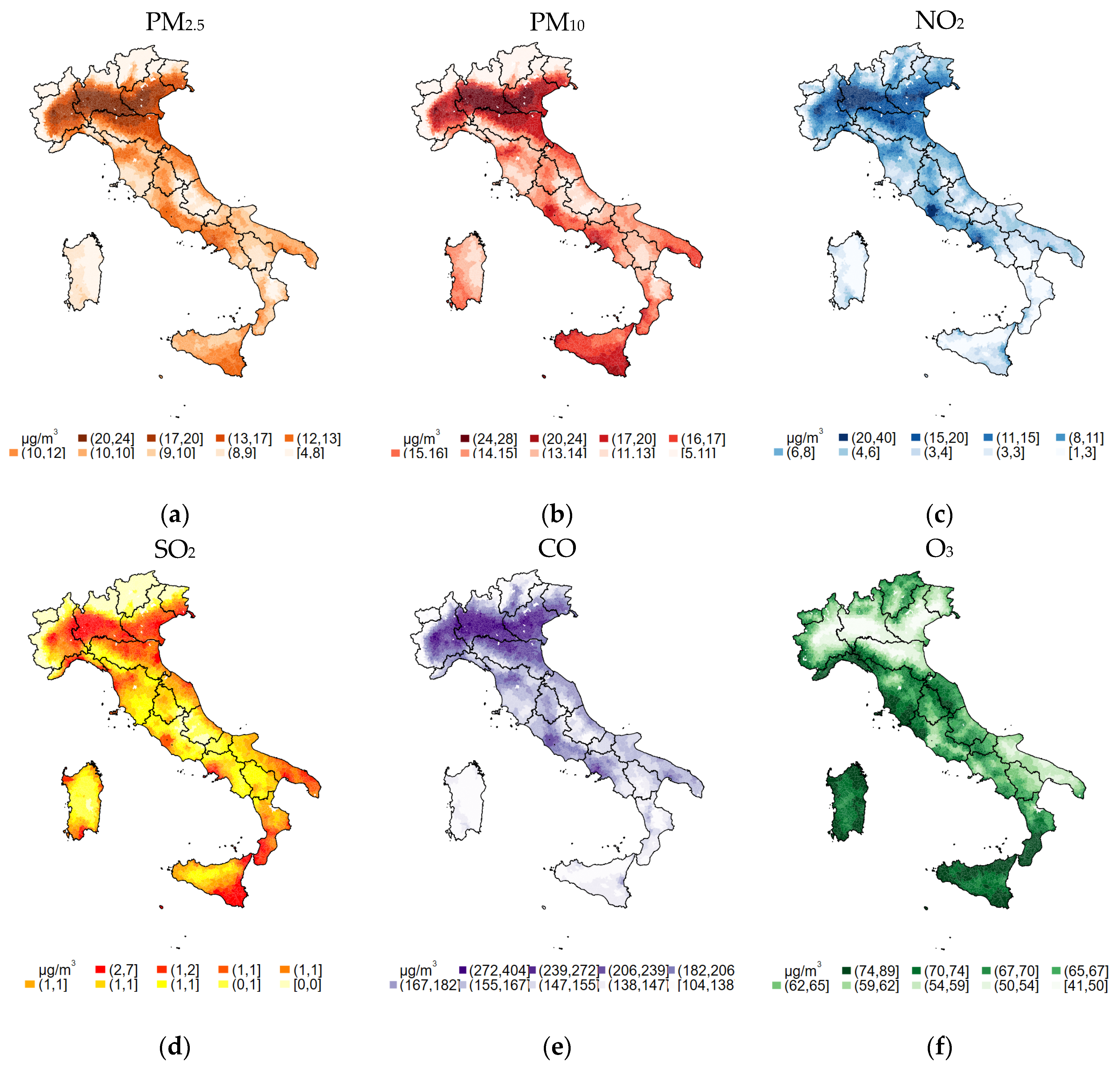
Figure 2.
The geographical distribution of national parks in Italy (as of 2020). Red dots indicate municipalities located in national parks.
Figure 2.
The geographical distribution of national parks in Italy (as of 2020). Red dots indicate municipalities located in national parks.
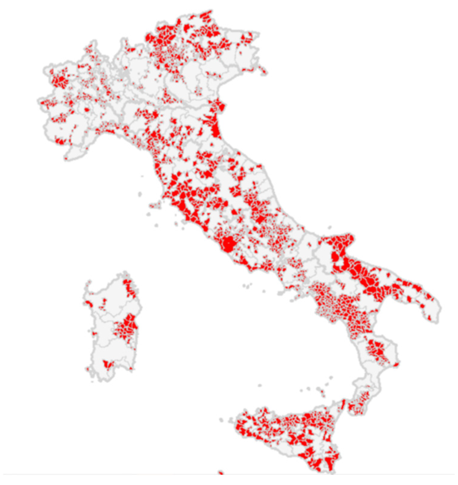
Figure 3.
The 95% confidence intervals of pollution levels in park vs. non-park municipalities. Note: the horizontal red line shows the average level of PM2.5 concentration advised by the WHO.
Figure 3.
The 95% confidence intervals of pollution levels in park vs. non-park municipalities. Note: the horizontal red line shows the average level of PM2.5 concentration advised by the WHO.

Figure 4.
Air quality in the 12 main Italian national parks—PM2.5. (a) Gargano and Alta Murgia; (b) Appennino Tosco Emiliano and Cinque Terre; (c) Aspromonte; (d) Foreste Casentinesi and Monte Falterona; (e) Cilento, Val d’Agri, Pollino and Sila; subfigure (f) Circeo; (g) Gran Paradiso; (h) Sibililini Gran Sasso Abbruzzi; subfigure (i) Stelvio; subfigure (j) Val Grande; (k) Dolomiti Bellunesi; subfigure (l) Gulf of Orosei and Gennergentu.

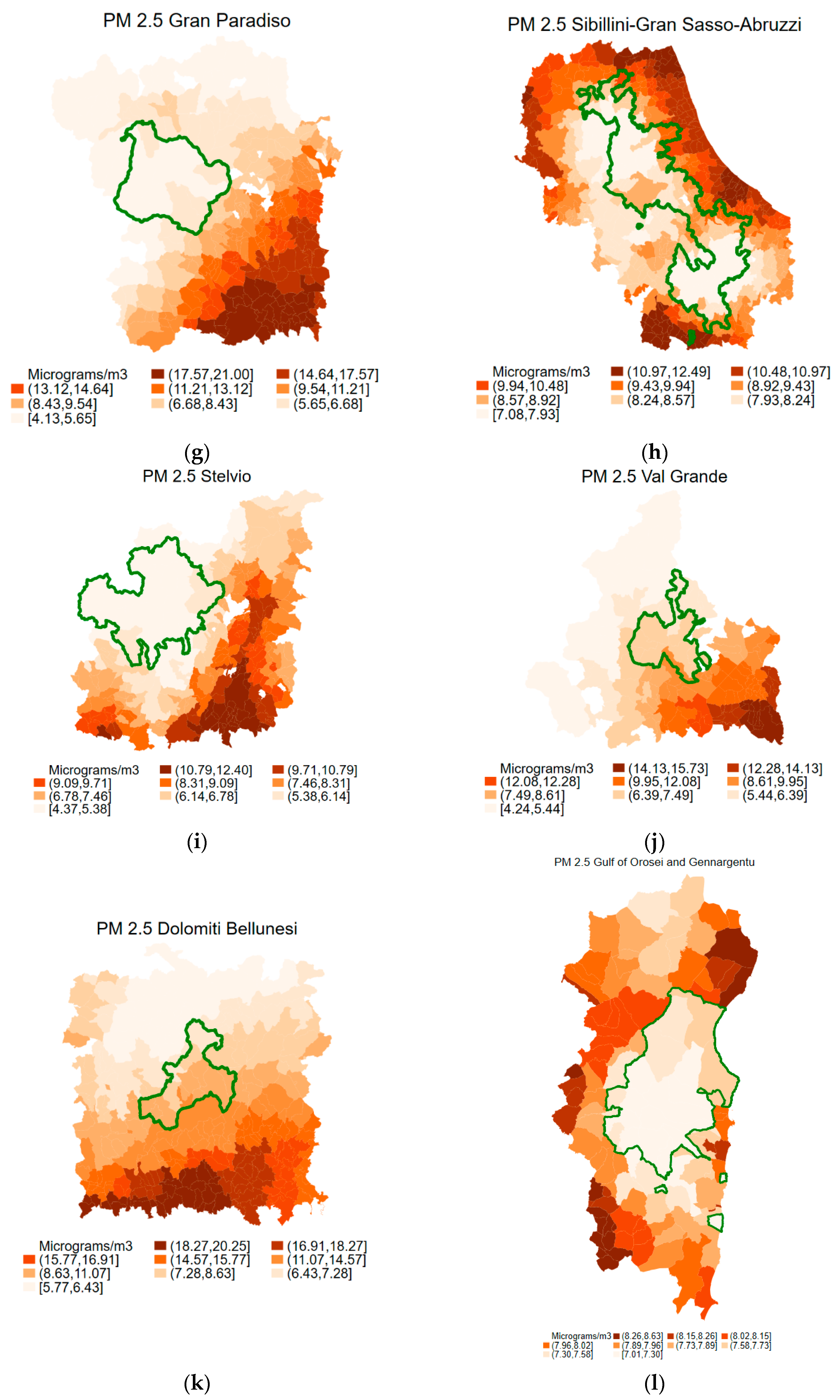
Table 1.
Variable legend.
| Variable | Description | Source |
|---|---|---|
| PM2.5 | Particulate matter with diameter < 2.5 µm (µg/m3). | Copernicus Atmospheric Monitoring Service |
| PM10 | Particulate matter with diameter < 10 µm (µg/m3). | Copernicus Atmospheric Monitoring Service |
| Nitrogen dioxide (NO2) | µg/m3 | Copernicus Atmospheric Monitoring Service |
| Sulphur dioxide (SO2) | µg/m3 | Copernicus Atmospheric Monitoring Service |
| Carbon monoxide (CO) | µg/m3 | Copernicus Atmospheric Monitoring Service |
| Ozone (O3) | µg/m3 | Copernicus Atmospheric Monitoring Service |
| Population | Number of residents in 2011 at the municipality level. | Italian National Statistical Institute |
| Employees | Number of employees operating in all economic sectors at the municipality level. | Italian National Statistical Institute |
| Density | Population per municipality area. | Italian National Statistical Institute |
| Over 65 | Share of people aged 65 or above. | Italian National Statistical Institute |
| Income | Total municipality gross income (million euros). | Italian National Statistical Institute |
| Precipitation | 11-day (from t−10 to t) moving average of total precipitation in mm at the municipality level. | Copernicus Climate Change Service |
| Wind | Wind intensity at 10 m from the ground (km/h). | Copernicus Climate Change Service |
| Radiation | Daily solar radiation (W/m2). | Copernicus Climate Change Service |
| Temperature | Air temperature measure at the height of 2 m above ground, at the municipality level. | Copernicus Climate Change Service |
| Park age | Distance from the year of park creation in years. | |
| Distance from park municipality | Distance between the given non-park municipality and the closest park municipality centroid. | |
| Region | Italian regions. | |
| Days since lockdown | Days since the start of the national lockdown, officially began on 10 March 2020. |
Table 2.
Descriptive statistics.
| Park Municipalities | Non-Park Municipalities | |||||
|---|---|---|---|---|---|---|
| Mean | 95% CI | Mean | 95% CI | |||
| PM2.5 # (µg/m3) | 8.709 | 8.692 | 8.727 | 12.818 | 12.811 | 12.825 |
| PM10 # (µg/m3) | 12.808 | 12.777 | 12.839 | 16.677 | 16.668 | 16.686 |
| NO2 # (µg/m3) | 3.252 | 3.243 | 3.262 | 9.788 | 9.780 | 9.795 |
| SO2 # (µg/m3) | 0.718 | 0.716 | 0.720 | 1.092 | 1.091 | 1.093 |
| CO # (µg/m3) | 145.898 | 145.798 | 145.997 | 196.962 | 196.894 | 197.031 |
| O3 # (µg/m3) | 68.423 | 68.381 | 68.465 | 62.277 | 62.260 | 62.294 |
| Population | 5514.589 | 5469.919 | 5559.259 | 7704.919 | 7672.863 | 7736.976 |
| Employees | 1065.349 | 1054.894 | 1075.805 | 2249.260 | 2235.537 | 2262.982 |
| Density | 112.518 | 111.557 | 113.479 | 316.219 | 315.710 | 316.728 |
| Days since lockdown | 3.952 | 3.910 | 3.995 | 3.952 | 3.941 | 3.963 |
| Precipitation * | 3.252 | 3.233 | 3.272 | 3.305 | 3.299 | 3.310 |
| Wind * | 6.291 | 6.277 | 6.304 | 6.300 | 6.297 | 6.303 |
| Radiation * | 178.413 | 5.14 | 359.985 | 168.404 | 2.985 | 369.60 |
| Park age | 34.44 | 11 | 98 | |||
| Distance from park municipality | 0.00719 | 0.00013 | 0.02341 | 0.00101 | 0.00012 | 0.01784 |
| Temperature * | 11.888 | 11.864 | 11.911 | 12.720 | 12.714 | 12.726 |
| Income | 57.444 | 56.899 | 57.989 | 108.921 | 108.319 | 109.523 |
* Contains modified Copernicus Climate Change Service Information (2017–2020), DOI: 10.24381/cds.e2161bac’. # Contains modified Copernicus Atmospheric Monitoring Service Information (2017–2020).
Table 3.
Correlation matrix of the variables used in the multivariate analysis (pairwise c+orrelation coefficients).
Table 3.
Correlation matrix of the variables used in the multivariate analysis (pairwise c+orrelation coefficients).
| PM2.5 | PM10 | NO2 | O3 | CO | SO2 | Population | Empl. | Density | Days | N.Park | Prec. | Wind | Temper. | Radiation | |
|---|---|---|---|---|---|---|---|---|---|---|---|---|---|---|---|
| PM2.5 | 1 | ||||||||||||||
| PM10 | 0.9193 | 1 | |||||||||||||
| NO2 | 0.6247 | 0.4639 | 1 | ||||||||||||
| O3 | −0.2547 | −0.1486 | −0.6405 | 1 | |||||||||||
| CO | 0.6926 | 0.5133 | 0.8966 | −0.5828 | 1 | ||||||||||
| SO2 | 0.5353 | 0.4563 | 0.5882 | −0.2470 | 0.5605 | 1 | |||||||||
| Population | 0.0295 | 0.0330 | 0.0749 | −0.0216 | 0.0463 | 0.0794 | 1 | ||||||||
| Employees | 0.0343 | 0.0311 | 0.0823 | −0.0280 | 0.0560 | 0.0705 | 0.9514 | 1 | |||||||
| Density | 0.1629 | 0.1418 | 0.3475 | −0.1026 | 0.2625 | 0.2914 | 0.2848 | 0.2449 | 1 | ||||||
| Days since lockdown | −0.0378 | 0.0010 | −0.1088 | 0.1643 | −0.0325 | −0.0243 | −0.0000 | −0.0000 | −0.0000 | 1 | |||||
| National Park | −0.1145 | −0.0831 | −0.1676 | 0.0694 | −0.1436 | −0.0956 | −0.0133 | −0.0168 | −0.0772 | −0.0000 | 1 | ||||
| Precipitation | −0.2174 | −0.2216 | −0.0583 | −0.0633 | −0.0827 | −0.1347 | −0.0074 | −0.0037 | 0.0018 | −0.0156 | −0.0017 | 1 | |||
| Wind | −0.2072 | −0.0909 | −0.1865 | 0.1400 | −0.1743 | 0.0335 | 0.0494 | 0.0227 | 0.0441 | 0.0122 | −0.0005 | 0.0437 | 1 | ||
| Temperature | 0.0624 | 0.1707 | −0.2554 | 0.4913 | −0.3544 | 0.0042 | 0.0347 | 0.0189 | 0.0637 | 0.0684 | −0.0258 | −0.0686 | 0.0569 | 1 | |
| Radiation | 0.0853 | 0.1603 | −0.3202 | 0.6707 | −0.3208 | −0.0301 | 0.0057 | −0.0009 | −0.0082 | 0.2209 | 0.0280 | −0.3118 | −0.0656 | 0.6754 | 1 |
Table 4.
The park municipality effect on air quality (OLS regressions: pollutant-dependent variables are the column headers).
Table 4.
The park municipality effect on air quality (OLS regressions: pollutant-dependent variables are the column headers).
| (1) | (2) | (3) | (4) | (5) | (6) | |
|---|---|---|---|---|---|---|
| PM2.5 | PM10 | NO2 | O3 | CO | SO2 | |
| Population | −8.45 × 10⁻⁶ *** | −8.62 × 10⁻⁶ *** | −2.22 × 10⁻⁵ *** | 4.33 × 10⁻⁶ | −0.000205 *** | −1.91 × 10⁻⁶ *** |
| (2.71 × 10⁻⁶) | (2.45 × 10⁻⁶) | (4.77 × 10⁻⁶) | (1.14 × 10⁻⁵) | (4.12 × 10⁻⁵) | (6.26 × 10⁻⁷) | |
| Employees | −3.88 × 10⁻⁵ ** | −3.40 × 10⁻⁵ ** | −0.000115 *** | 7.29 × 10⁻⁵ * | −0.000866 *** | −1.28 × 10⁻⁵ ** |
| (1.62 × 10⁻⁵) | (1.55 × 10⁻⁵) | (3.17 × 10⁻⁵) | (4.43 × 10⁻⁵) | (0.000253) | (5.59 × 10⁻⁶) | |
| Density | 0.00113 *** | 0.00115 *** | 0.00387 *** | −0.00265 *** | 0.0258 *** | 0.000340 *** |
| (0.000109) | (0.000108) | (0.000289) | (0.000223) | (0.00219) | (2.76 × 10⁻⁵) | |
| Day since lockdown | −0.0508 *** | −0.0406 *** | −0.0388 *** | 0.0137 *** | 0.0249 *** | −0.00139 *** |
| (0.000456) | (0.000553) | (0.000557) | (0.00143) | (0.00578) | (0.000105) | |
| Park municipality | −1.009 *** | −0.671 *** | −1.807 *** | 3.255 *** | −17.54 *** | −0.0918 *** |
| (0.133) | (0.137) | (0.182) | (0.234) | (1.614) | (0.0183) | |
| Rain | −0.154 *** | −0.192 *** | −0.0989 *** | 0.191 *** | −1.016 *** | −0.0103 *** |
| (0.00144) | (0.00189) | (0.00145) | (0.00234) | (0.0139) | (0.000129) | |
| Wind | −0.477 *** | −0.400 *** | −0.312 *** | 0.877 *** | −3.430 *** | −0.000917 |
| (0.00894) | (0.0107) | (0.00879) | (0.0114) | (0.0889) | (0.000968) | |
| Temperature | 0.699 *** | 1.021 *** | 0.399 *** | 0.0429 * | 2.494 *** | 0.0397 *** |
| (0.0108) | (0.0104) | (0.0176) | (0.0248) | (0.174) | (0.00167) | |
| Radiation | 0.0143 *** | 0.0181 *** | −0.0103 *** | 0.0848 *** | −0.0821 *** | 0.00129 *** |
| (0.000239) | (0.000222) | (0.000348) | (0.000730) | (0.00378) | (3.83 × 10⁻⁵) | |
| Income | 0.00136 *** | 0.00126 *** | 0.00391 *** | −0.00214 | 0.0308 *** | 0.000408 ** |
| (0.000474) | (0.000433) | (0.000905) | (0.00148) | (0.00729) | (0.000159) | |
| Valle d’Aosta | −2.264 *** | −0.957 *** | −3.472 *** | 4.803 *** | −56.31 *** | −0.387 *** |
| (0.218) | (0.247) | (0.305) | (0.546) | (2.838) | (0.0267) | |
| Lombardia | 3.399 *** | 3.559 *** | 5.734 *** | −4.112 *** | 50.23 *** | 0.435 *** |
| (0.214) | (0.214) | (0.347) | (0.401) | (2.909) | (0.0377) | |
| Trentino Alto-Adige | −2.651 *** | −1.980 *** | −3.580 *** | 6.584 *** | −38.37 *** | −0.500 *** |
| 3 | (0.160) | (0.196) | (0.236) | (0.422) | (2.286) | (0.0201) |
| Veneto | 2.870 *** | 3.089 *** | 2.540 *** | −4.272 *** | 24.92 *** | 0.0488 ** |
| (0.206) | (0.210) | (0.305) | (0.458) | (2.507) | (0.0248) | |
| Friuli-Venezia Giulia | −1.550 *** | −1.955 *** | −2.162 *** | −2.083 *** | −20.20 *** | −0.0619 * |
| (0.164) | (0.143) | (0.285) | (0.624) | (2.361) | (0.0346) | |
| Liguria | −3.654 *** | −4.159 *** | −4.660 *** | 12.09 *** | −34.19 *** | −0.0913 * |
| (0.211) | (0.232) | (0.278) | (0.294) | (2.172) | (0.0515) | |
| Emilia-Romagna | −0.194 | 0.00534 | −0.208 | −1.937 *** | −5.215 * | −0.0775 *** |
| (0.242) | (0.233) | (0.394) | (0.751) | (2.980) | (0.0263) | |
| Toscana | −4.207 *** | −3.961 *** | −4.988 *** | 7.318 *** | −35.48 *** | −0.264 *** |
| (0.130) | (0.138) | (0.244) | (0.361) | (1.933) | (0.0265) | |
| Umbria | −4.160 *** | −3.781 *** | −5.037 *** | 6.192 *** | −41.81 *** | −0.417 *** |
| (0.136) | (0.134) | (0.244) | (0.442) | (1.911) | (0.0216) | |
| Marche | −3.324 *** | −3.132 *** | −5.234 *** | 7.030 *** | −36.56 *** | −0.239 *** |
| (0.155) | (0.159) | (0.217) | (0.379) | (1.782) | (0.0226) | |
| Lazio | −4.670 *** | −4.322 *** | −4.427 *** | 4.525 *** | −37.12 *** | −0.550 *** |
| (0.113) | (0.107) | (0.226) | (0.327) | (1.759) | (0.0192) | |
| Abruzzo | −4.746 *** | −4.382 *** | −5.715 *** | 4.561 *** | −45.65 *** | −0.436 *** |
| (0.121) | (0.118) | (0.204) | (0.302) | (1.783) | (0.0202) | |
| Molise | −4.401 *** | −4.082 *** | −6.717 *** | 4.753 *** | −47.74 *** | −0.496 *** |
| (0.114) | (0.114) | (0.195) | (0.474) | (1.666) | (0.0187) | |
| Campania | −3.952 *** | −3.214 *** | −5.193 *** | 3.676 *** | −38.41 *** | −0.458 *** |
| (0.131) | (0.129) | (0.249) | (0.304) | (1.925) | (0.0231) | |
| Puglia | −4.162 *** | −4.209 *** | −6.561 *** | −8.733 *** | −32.08 *** | −0.154 *** |
| (0.143) | (0.153) | (0.226) | (0.486) | (1.911) | (0.0293) | |
| Basilicata | −5.259 *** | −4.987 *** | −7.374 *** | −0.979 ** | −50.04 *** | −0.418 *** |
| (0.153) | (0.187) | (0.217) | (0.450) | (1.742) | (0.0250) | |
| Calabria | −5.228 *** | −4.300 *** | −7.969 *** | 6.286 *** | −52.65 *** | 0.138 *** |
| (0.125) | (0.133) | (0.206) | (0.355) | (1.631) | (0.0402) | |
| Sicilia | −5.326 *** | −3.451 *** | −8.634 *** | 9.605 *** | −67.86 *** | 0.117 * |
| (0.128) | (0.132) | (0.241) | (0.342) | (1.883) | (0.0700) | |
| Sardegna | −6.386 *** | −5.359 *** | −7.848 *** | 6.401 *** | −60.45 *** | −0.521 *** |
| (0.121) | (0.123) | (0.207) | (0.301) | (1.672) | (0.0272) | |
| Monday | −0.0745 *** | 0.146 *** | 0.790 *** | −1.545 *** | 2.630 *** | 0.0165 *** |
| (0.0124) | (0.0168) | (0.0120) | (0.0161) | (0.0840) | (0.00134) | |
| Tuesday | −0.219 *** | −0.0389 ** | 1.030 *** | −1.929 *** | 2.782 *** | 0.0588 *** |
| (0.0142) | (0.0168) | (0.0139) | (0.0244) | (0.0895) | (0.00156) | |
| Wednesday | −0.119 *** | −0.0999 *** | 1.449 *** | −1.614 *** | 4.337 *** | 0.0777 *** |
| (0.0106) | (0.0126) | (0.0182) | (0.0212) | (0.0851) | (0.00174) | |
| Thursday | 0.227 *** | 0.349 *** | 1.826 *** | −1.777 *** | 6.640 *** | 0.109 *** |
| (0.00909) | (0.0114) | (0.0258) | (0.0238) | (0.123) | (0.00216) | |
| Friday | 0.542 *** | 0.747 *** | 1.992 *** | −1.992 *** | 8.526 *** | 0.114 *** |
| (0.00994) | (0.0131) | (0.0290) | (0.0234) | (0.155) | (0.00225) | |
| Saturday | 0.209 *** | 0.224 *** | 0.970 *** | −1.276 *** | 3.068 *** | 0.0496 *** |
| (0.00637) | (0.00742) | (0.0161) | (0.0190) | (0.0785) | (0.000962) | |
| February | 0.692 *** | −0.0135 | −1.868 *** | 6.206 *** | 4.793 *** | −0.0903 *** |
| (0.0182) | (0.0222) | (0.0359) | (0.0548) | (0.304) | (0.00190) | |
| March | −2.391 *** | −3.308 *** | −5.408 *** | 11.46 *** | −23.09 *** | −0.395 *** |
| (0.0590) | (0.0605) | (0.0804) | (0.0903) | (0.741) | (0.00645) | |
| April | −3.600 *** | −4.898 *** | −9.075 *** | 18.51 *** | −59.50 *** | −0.569 *** |
| (0.101) | (0.108) | (0.140) | (0.151) | (1.235) | (0.0113) | |
| May | −11.43 *** | −14.89 *** | −10.89 *** | 14.24 *** | −91.93 *** | −1.023 *** |
| (0.140) | (0.144) | (0.179) | (0.192) | (1.581) | (0.0142) | |
| June | −14.83 *** | −18.42 *** | −13.96 *** | 17.46 *** | −129.0 *** | −1.213 *** |
| (0.189) | (0.183) | (0.259) | (0.325) | (2.339) | (0.0241) | |
| July | −17.79 *** | −23.02 *** | −15.44 *** | 23.74 *** | −144.7 *** | −1.428 *** |
| (0.215) | (0.210) | (0.297) | (0.378) | (2.694) | (0.0282) | |
| August | −17.70 *** | −23.21 *** | −15.87 *** | 17.04 *** | −137.0 *** | −1.354 *** |
| (0.213) | (0.204) | (0.304) | (0.356) | (2.797) | (0.0275) | |
| September | −13.49 *** | −17.69 *** | −13.24 *** | 9.692 *** | −106.6 *** | −1.009 *** |
| (0.157) | (0.147) | (0.245) | (0.278) | (2.245) | (0.0218) | |
| October | −8.668 *** | −11.48 *** | −9.739 *** | −0.357 * | −96.37 *** | −0.592 *** |
| (0.119) | (0.111) | (0.187) | (0.205) | (1.745) | (0.0171) | |
| November | −5.894 *** | −7.680 *** | −5.459 *** | −5.441 *** | −65.13 *** | −0.402 *** |
| (0.0737) | (0.0706) | (0.107) | (0.121) | (0.980) | (0.00881) | |
| December | −0.989 *** | −1.060 *** | −0.950 *** | −6.117 *** | −14.83 *** | −0.132 *** |
| (0.0227) | (0.0264) | (0.0367) | (0.0529) | (0.337) | (0.00561) | |
| Constant | 13.43 *** | 13.95 *** | 16.24 *** | 33.10 *** | 269.2 *** | 0.947 *** |
| (0.169) | (0.177) | (0.236) | (0.352) | (2.243) | (0.0180) | |
| Observations | 6,899,886 | 6,899,886 | 6,899,886 | 6,899,886 | 6,899,886 | 6,899,886 |
| R-squared | 0.351 | 0.280 | 0.550 | 0.620 | 0.509 | 0.276 |
Robust standard errors are clustered at the municipality level. *** p < 0.01, ** p < 0.05, * p < 0.1.
Table 5.
Robustness checks.
| Panel A. National parks and air quality—monitoring points with distance from municipality centroid < 5 km. | ||||||
| (1) | (2) | (3) | (4) | (5) | (6) | |
| PM2.5 | PM10 | NO2 | O3 | CO | SO2 | |
| Park Municipality | −1.059 *** | −0.722 *** | −1.858 *** | 3.359 *** | −18.15 *** | −0.0965 *** |
| (0.149) | (0.153) | (0.201) | (0.259) | (1.792) | (0.0202) | |
| Observations | 5,275,242 | 5,275,242 | 5,275,242 | 5,275,242 | 5,275,242 | 5,275,242 |
| R-squared | 0.353 | 0.283 | 0.551 | 0.621 | 0.510 | 0.281 |
| *** p < 0.01. Full estimate results are omitted for reasons of space and available upon request. | ||||||
| Panel B. National parks and air quality, controlling for time trend. | ||||||
| (1) | (2) | (3) | (4) | (5) | (6) | |
| PM2.5 | PM10 | NO2 | O3 | CO | SO2 | |
| Park Municipality | −0.428 *** | −0.0195 | −2.063 *** | 2.638 *** | −12.44 *** | −0.223 *** |
| (0.145) | (0.153) | (0.183) | (0.244) | (1.678) | (0.0216) | |
| Park Age | −0.0013 *** | −0.0015 *** | 0.00059 *** | 0.00143 *** | −0.0116 *** | 0.000300 *** |
| (6.41 × 10⁻⁵) | (8.11 × 10⁻⁵) | (6.61 × 10⁻⁵) | (0.00034) | (0.000629) | (1.78 × 10⁻⁵) | |
| Time | 0.00158 *** | 0.00306 *** | −0.000999 *** | −0.00367 *** | 0.0101 *** | −0.000311 *** |
| (3.61 × 10⁻⁵) | (4.63 × 10⁻⁵) | (5.43 × 10⁻⁵) | (0.000124) | (0.000472) | (9.97 × 10⁻⁶) | |
| Observations | 5,275,242 | 5,275,242 | 5,275,242 | 5,275,242 | 5,275,242 | 5,275,242 |
| R-squared | 0.354 | 0.287 | 0.552 | 0.623 | 0.510 | 0.286 |
| *** p < 0.01. Full estimate results are omitted for reasons of space and available upon request. | ||||||
| Panel C. National parks and air quality, controlling for time trend—monitoring posts with distance from municipality centroid < 5 km | ||||||
| (1) | (2) | (3) | (4) | (5) | (6) | |
| PM2.5 | PM10 | NO2 | O3 | CO | SO2 | |
| Park Municipality | −0.467 *** | −0.0588 | −2.109 *** | 2.723 *** | −12.91 *** | −0.228 *** |
| (0.161) | (0.171) | (0.203) | (0.270) | (1.863) | (0.0238) | |
| Park Age | −0.0014 *** | −0.0015 *** | 0.000576 *** | 0.00147 *** | −0.0120 *** | 0.000301 *** |
| (7.12 × 10⁻⁵) | (8.99 × 10⁻⁵) | (7.29 × 10⁻⁵) | (0.000376) | (0.000699) | (1.95 × 10⁻⁵) | |
| Time | 0.00160 *** | 0.00309 *** | −0.00101 *** | −0.00369 *** | 0.0102 *** | −0.000314 *** |
| (4.02 × 10⁻⁵) | (5.14 × 10⁻⁵) | (6.04 × 10⁻⁵) | (0.000139) | (0.000526) | (1.11 × 10⁻⁵) | |
| Observations | 5,275,242 | 5,275,242 | 5,275,242 | 5,275,242 | 5,275,242 | 5,275,242 |
| R-squared | 0.354 | 0.287 | 0.552 | 0.623 | 0.510 | 0.286 |
| *** p < 0.01. Full estimate results are omitted for reasons of space and available upon request. | ||||||
| Panel D. National parks and air quality—excluding the lockdown period | ||||||
| (1) | (2) | (3) | (4) | (5) | (6) | |
| PM2.5 | PM10 | NO2 | O3 | CO | SO2 | |
| Park Municipality | −1.023 *** | −0.756 *** | −1.864 *** | 3.373 *** | −17.96 *** | −0.0905 *** |
| (0.137) | (0.142) | (0.189) | (0.239) | (1.679) | (0.0187) | |
| Observations | 6,250,577 | 6,250,577 | 6,250,577 | 6,250,577 | 6,250,577 | 6,250,577 |
| R-squared | 0.343 | 0.289 | 0.551 | 0.624 | 0.505 | 0.275 |
| *** p < 0.01. Full estimate results are omitted for reasons of space and available upon request. | ||||||
| Panel E. National parks and air quality—excluding the lockdown period, monitoring posts with distance from municipality centroid < 5 km | ||||||
| (1) | (2) | (3) | (4) | (5) | (6) | |
| PM2.5 | PM10 | NO2 | O3 | CO | SO2 | |
| Park Municipality | −1.075 *** | −0.808 *** | −1.918 *** | 3.478 *** | −18.60 *** | −0.0955 *** |
| (0.153) | (0.159) | (0.209) | (0.264) | (1.864) | (0.0206) | |
| Observations | 4,778,819 | 4,778,819 | 4,778,819 | 4,778,819 | 4,778,819 | 4,778,819 |
| R-squared | 0.345 | 0.292 | 0.553 | 0.624 | 0.506 | 0.280 |
| *** p < 0.01. Full estimate results are omitted for reasons of space and available upon request. | ||||||
| Panel F. National parks and air quality, controlling for the distance from park municipality—excluding park municipalities | ||||||
| (1) | (2) | (3) | (4) | (5) | (6) | |
| PM2.5 | PM10 | NO2 | O3 | CO | SO2 | |
| Distance from Park Municipality | −449.4 *** | −422.8 *** | −645.1 *** | 614.6 *** | −6051 *** | −41.28 *** |
| (37.23) | (37.05) | (64.57) | (85.22) | (545.5) | (6.253) | |
| Observations | 6,458,004 | 6,458,004 | 6,458,004 | 6,458,004 | 6,458,004 | 6,458,004 |
| R-squared | 0.351 | 0.281 | 0.550 | 0.632 | 0.512 | 0.273 |
| *** p < 0.01. Full estimate results are omitted for reasons of space and available upon request | ||||||
| Panel G. National parks and air quality, controlling for the distance from park municipality—excluding park municipalities, monitoring posts with distance from municipality centroid < 5 km | ||||||
| (1) | (2) | (3) | (4) | (5) | (6) | |
| PM2.5 | PM10 | NO2 | O3 | CO | SO2 | |
| Distance from Park Municipality | −470.6 *** | −445.7 *** | −681.1 *** | 626.8 *** | −6369 *** | −45.38 *** |
| (43.52) | (43.41) | (75.37) | (97.71) | (636.7) | (7.211) | |
| Observations | 4,940,964 | 4,940,964 | 4,940,964 | 4,940,964 | 4,940,964 | 4,940,964 |
| R-squared | 0.353 | 0.284 | 0.553 | 0.632 | 0.513 | 0.279 |
| *** p < 0.01. Full estimate results are omitted for reasons of space and available upon request | ||||||
| Panel H. National parks and air quality, controlling for time trend and the distance from park municipality—excluding park municipalities | ||||||
| (1) | (2) | (3) | (4) | (5) | (6) | |
| PM2.5 | PM10 | NO2 | O3 | CO | SO2 | |
| Distance from Park Municipality | −317.5 *** | −277.1 *** | −732.1 *** | 480.6 *** | −4242 *** | −83.40 *** |
| (33.64) | (32.90) | (68.78) | (79.76) | (484.2) | (7.723) | |
| Distance × Time | −0.303 *** | −0.337 *** | 0.200 *** | 0.312 *** | −4.130 *** | 0.0963 *** |
| (0.0233) | (0.0265) | (0.0253) | (0.0807) | (0.358) | (0.00784) | |
| Time | 0.00189 *** | 0.00345 *** | −0.00118 *** | −0.00394 *** | 0.0141 *** | −0.000409 *** |
| (4.84 × 10⁻⁵) | (5.97 × 10⁻⁵) | (6.91 × 10⁻⁵) | (0.000160) | (0.000684) | (1.19 × 10⁻⁵) | |
| Observations | 6,458,004 | 6,458,004 | 6,458,004 | 6,458,004 | 6,458,004 | 6,458,004 |
| R-squared | 0.353 | 0.284 | 0.551 | 0.633 | 0.513 | 0.279 |
| *** p < 0.01. Full estimate results are omitted for reasons of space and available upon request | ||||||
| Panel I. National parks and air quality, controlling for time trend and the distance from park municipality—excluding park municipalities, monitoring points with distance from municipality centroid < 5 km | ||||||
| (1) | (2) | (3) | (4) | (5) | (6) | |
| PM2.5 | PM10 | NO2 | O3 | CO | SO2 | |
| Distance from Park Municipality | −336.3 *** | −295.3 *** | −769.5 *** | 490.8 *** | −4525 *** | −87.61 *** |
| (39.29) | (38.40) | (80.18) | (91.41) | (563.4) | (8.915) | |
| Distance × Park Municipality × Time | −0.309 *** | −0.348 *** | 0.203 *** | 0.317 *** | −4.211 *** | 0.0966 *** |
| (0.0263) | (0.0301) | (0.0286) | (0.0916) | (0.407) | (0.00883) | |
| Time | 0.00192 *** | 0.00349 *** | −0.00119 *** | −0.00396 *** | 0.0143 *** | −0.000412 *** |
| (5.40 × 10⁻⁵) | (6.65 × 10⁻⁵) | (7.70 × 10⁻⁵) | (0.000178) | (0.000765) | (1.32 × 10⁻⁵) | |
| Observations | 4,940,964 | 4,940,964 | 4,940,964 | 4,940,964 | 4,940,964 | 4,940,964 |
| R-squared | 0.355 | 0.288 | 0.553 | 0.634 | 0.514 | 0.285 |
| *** p < 0.01. Full estimate results are omitted for reasons of space and available upon request | ||||||
| Panel J. National parks and air quality, controlling for time trend and the distance from park municipality—excluding park municipalities and distances above the 40th centile | ||||||
| (1) | (2) | (3) | (4) | (5) | (6) | |
| PM2.5 | PM10 | NO2 | O3 | CO | SO2 | |
| Distance from Park Municipality | −123.1 *** | −73.82 *** | −73.82 *** | 259.5 *** | −2622 *** | −20.03 *** |
| (17.25) | (20.23) | (20.23) | (56.45) | (257.1) | (5.883) | |
| Distance × Time | −0.0365 ** | −0.0551 *** | −0.0551 *** | −0.113 | 0.717 *** | 0.0236 *** |
| (0.0149) | (0.0186) | (0.0186) | (0.0790) | (0.156) | (0.00716) | |
| Time | 0.000996 *** | 0.00219 *** | 0.00219 *** | −0.00166 *** | −0.000876 * | −4.17 × 10⁻⁵ ** |
| (5.53 × 10⁻⁵) | (7.09 × 10⁻⁵) | (7.09 × 10⁻⁵) | (0.000206) | (0.000504) | (1.81 × 10⁻⁵) | |
| Observations | 2,205,000 | 2,205,000 | 2,205,000 | 2,205,000 | 2,205,000 | 2,205,000 |
| R-squared | 0.343 | 0.283 | 0.283 | 0.588 | 0.510 | 0.327 |
| *** p < 0.01, ** p < 0.05, * p < 0.1. Full estimate results are omitted for reasons of space and available upon request | ||||||
Table 6.
Average impact on mortality of pollutants considered in our study.
| Pollutant | % Change in Risk (95% CI) in Mortality Associated with a 10 μg/m3 Increase | |
|---|---|---|
| (1) | (2) | |
| Mean of the Appendix Studies | Mean of the Appendix Studies (Excluding the Minimum and Maximum Value) | |
| PM2.5 | 9.67 (0.6, 20) | 10.23 (2.7, 18.8) |
| PM10 | 17.17 (7.1, 28.5) | 13 (0.2, 27.7) |
| NO2 | 6.30 (0.5, 12) | 6.5 (1.3, 11.3) |
| SO2 | 1.45 (1, 1.73) | 1.01 (0.7, 1.2) |
| O3 | 1.09 (0.5, 1.6) | 1.07 (0.5, 1.7) |
| CM | 28.23 (17.7, 38.7) | 20.45 (11.5, 29.4) |
Empirical studies are those listed in Appendix A. The column (1) is the simple mean, while the column (2) is the mean dropping the two extreme values (the minimum and the maximum, respectively).
Disclaimer/Publisher’s Note: The statements, opinions and data contained in all publications are solely those of the individual author(s) and contributor(s) and not of MDPI and/or the editor(s). MDPI and/or the editor(s) disclaim responsibility for any injury to people or property resulting from any ideas, methods, instructions or products referred to in the content. |
© 2023 by the authors. Licensee MDPI, Basel, Switzerland. This article is an open access article distributed under the terms and conditions of the Creative Commons Attribution (CC BY) license (https://creativecommons.org/licenses/by/4.0/).
Share and Cite
MDPI and ACS Style
Becchetti, L.; Beccari, G.; Conzo, G.; De Santis, D.; Conzo, P.; Salustri, F. The Green Lung: National Parks and Air Quality in Italian Municipalities. Sustainability 2023, 15, 7802. https://doi.org/10.3390/su15107802
AMA Style
Becchetti L, Beccari G, Conzo G, De Santis D, Conzo P, Salustri F. The Green Lung: National Parks and Air Quality in Italian Municipalities. Sustainability. 2023; 15(10):7802. https://doi.org/10.3390/su15107802
Chicago/Turabian StyleBecchetti, Leonardo, Gabriele Beccari, Gianluigi Conzo, Davide De Santis, Pierluigi Conzo, and Francesco Salustri. 2023. "The Green Lung: National Parks and Air Quality in Italian Municipalities" Sustainability 15, no. 10: 7802. https://doi.org/10.3390/su15107802
Note that from the first issue of 2016, this journal uses article numbers instead of page numbers. See further details here.