
Green Space Quality Analysis Using Machine Learning Approaches


Abstract
1. Introduction
1.1. Research Motivation
1.2. Research Contributions
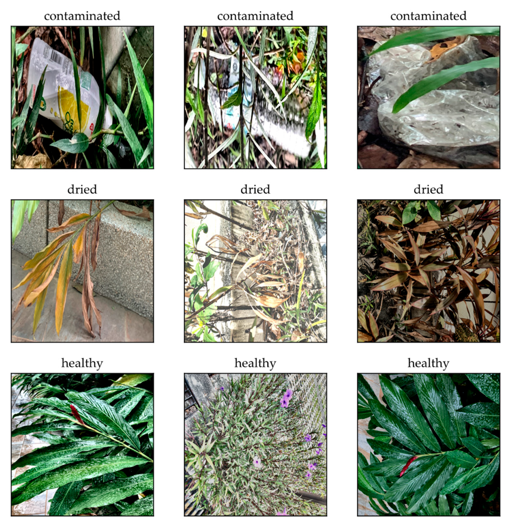
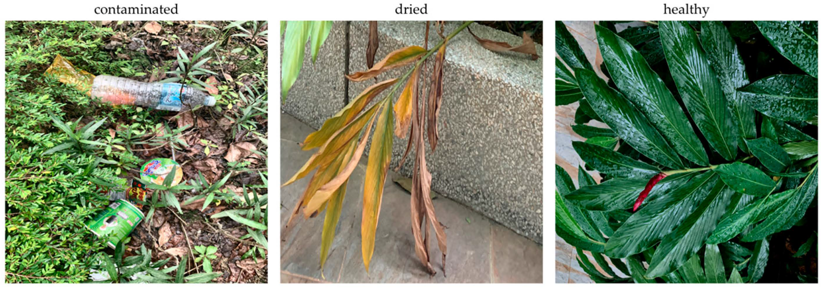
- Construct a green space image dataset comprising three classes: contaminated, healthy, and dried.
- Perform image augmentation techniques to balance the green space image dataset.
- Develop nine image classification models using transfer learning to classify green space images.
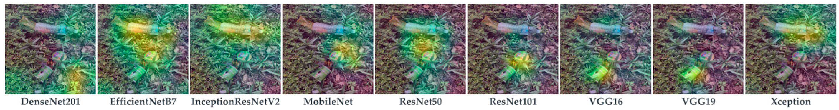
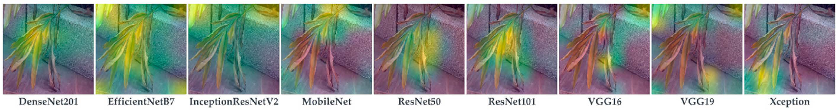
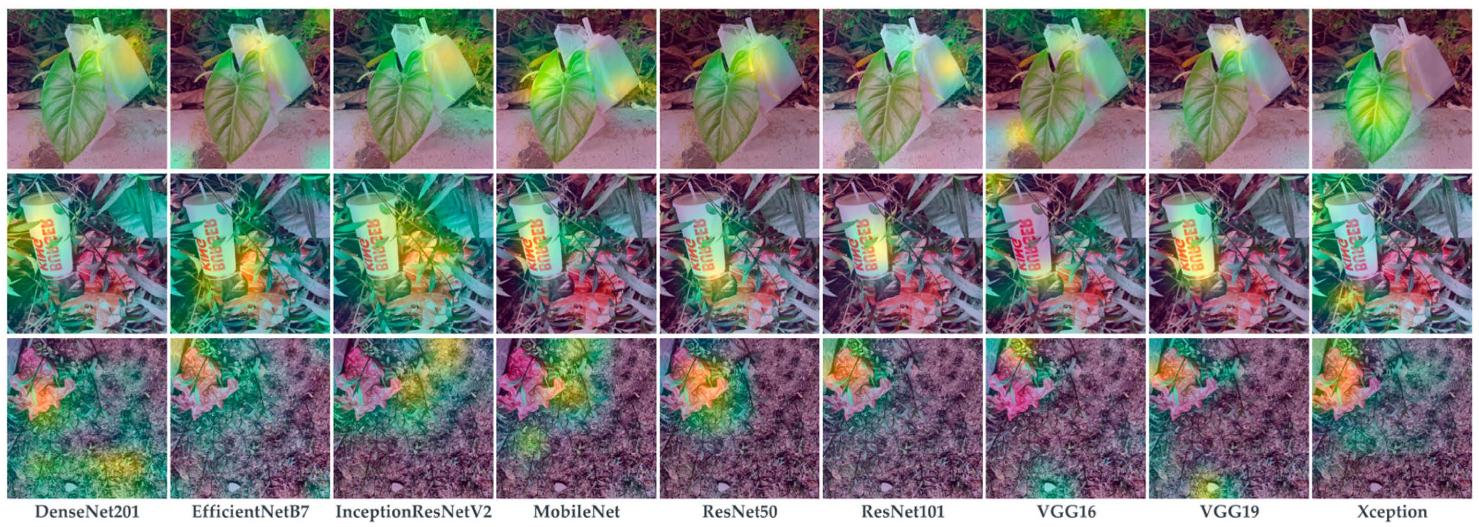
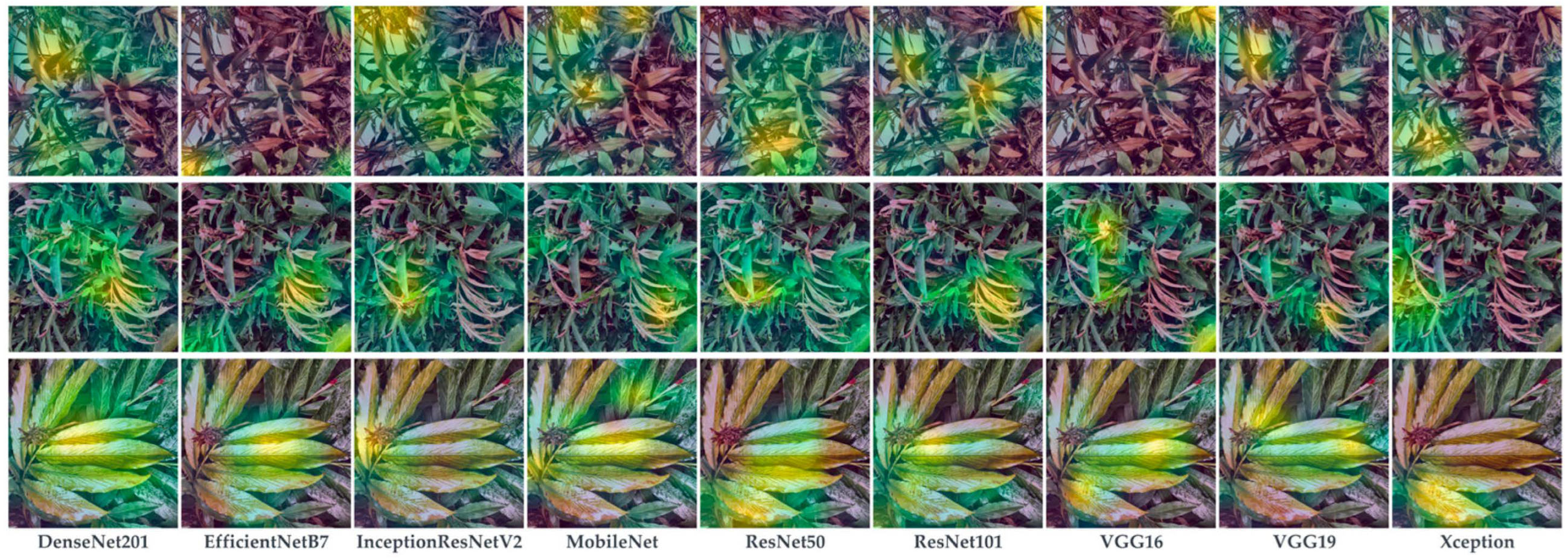
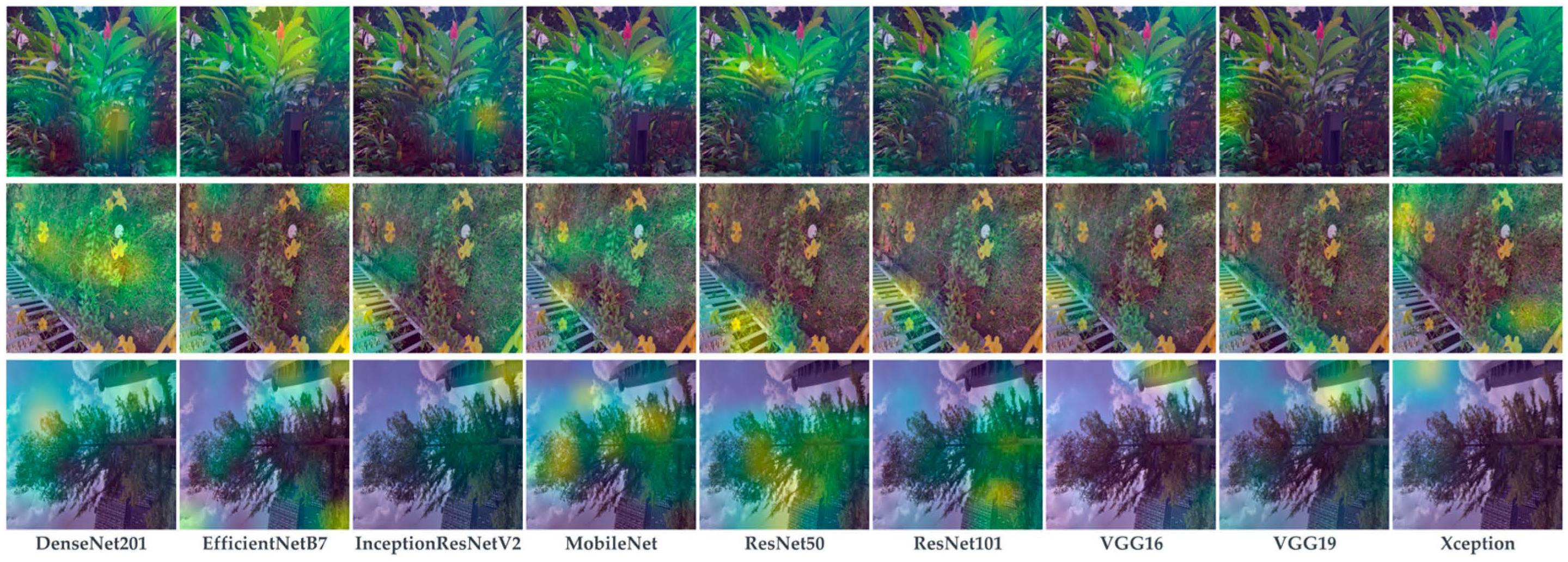
- Evaluate the learning performance of developed models using Grad-CAM.
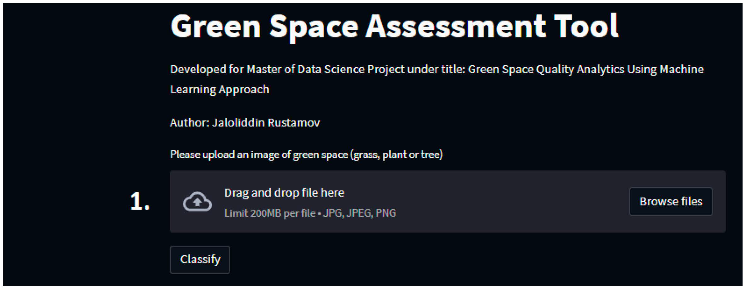
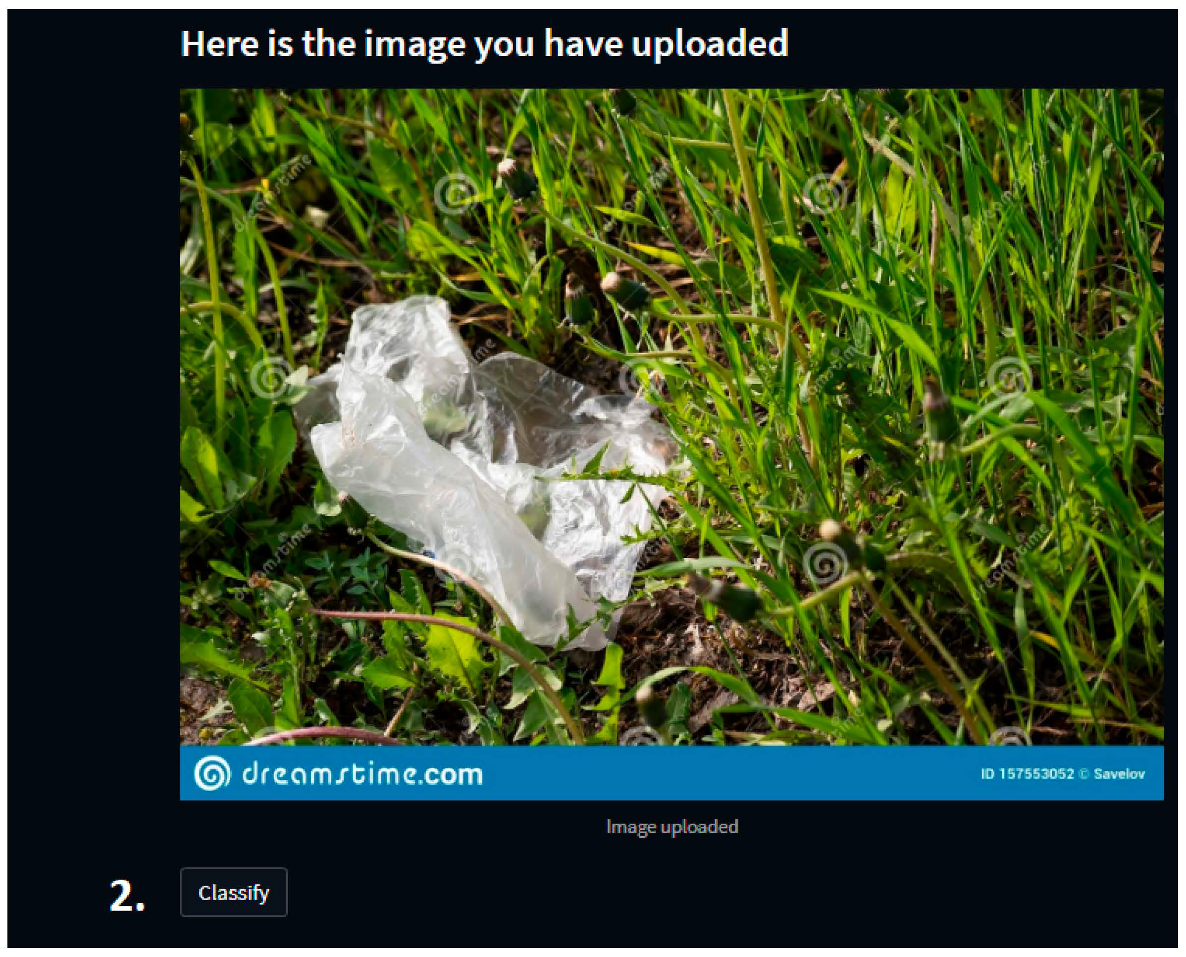
- Deploy the best-performing image classification model on the Streamlit cloud-based framework for public use.
1.3. Section Organization
2. Literature Review
2.1. Green Space Quality Analysis Using Traditional Methods
2.2. Green Space Quality Analysis Using Machine Learning
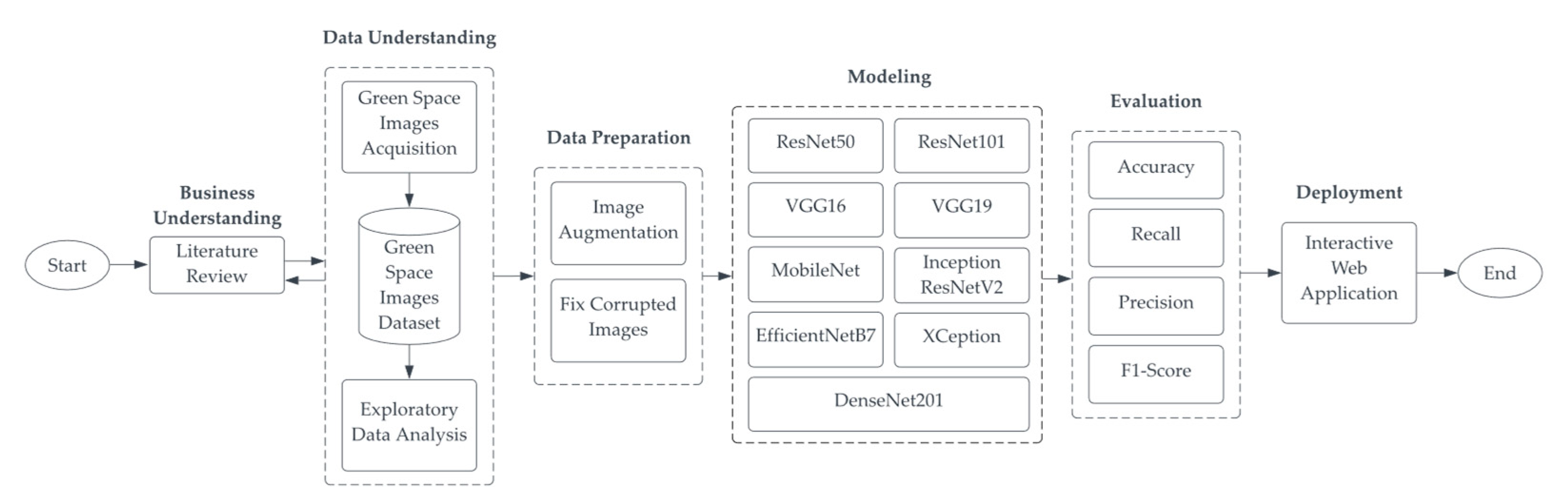
3. Methodology
3.1. Description of Dataset
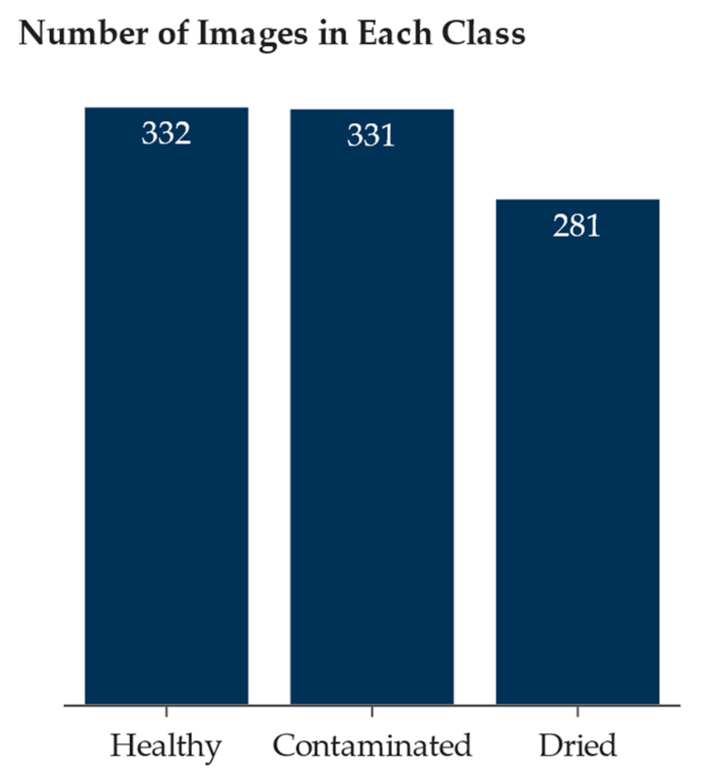
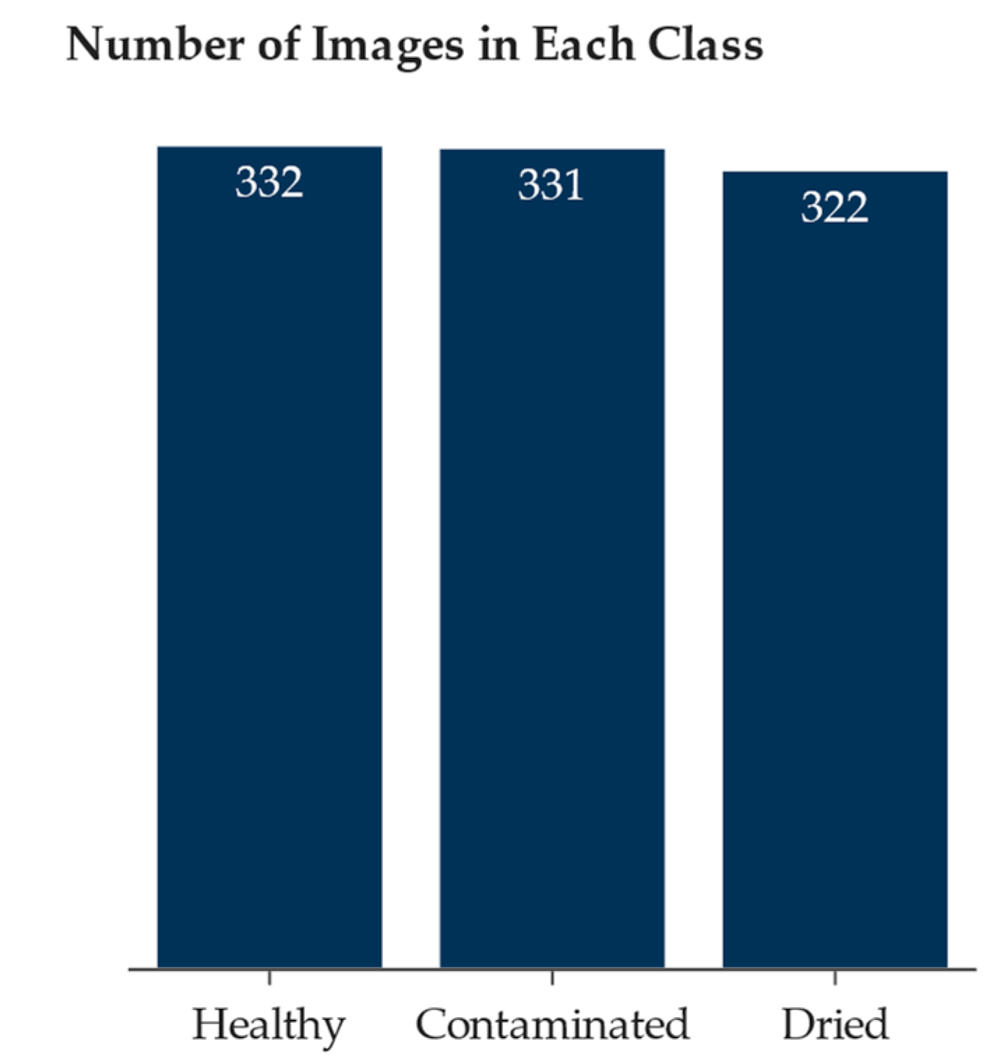
3.2. Exploratory Data Analysis
3.3. Data Pre-Processing
3.4. Model Training
3.5. Transfer Learning
3.6. Classification Models
3.7. Evaluation Metrics
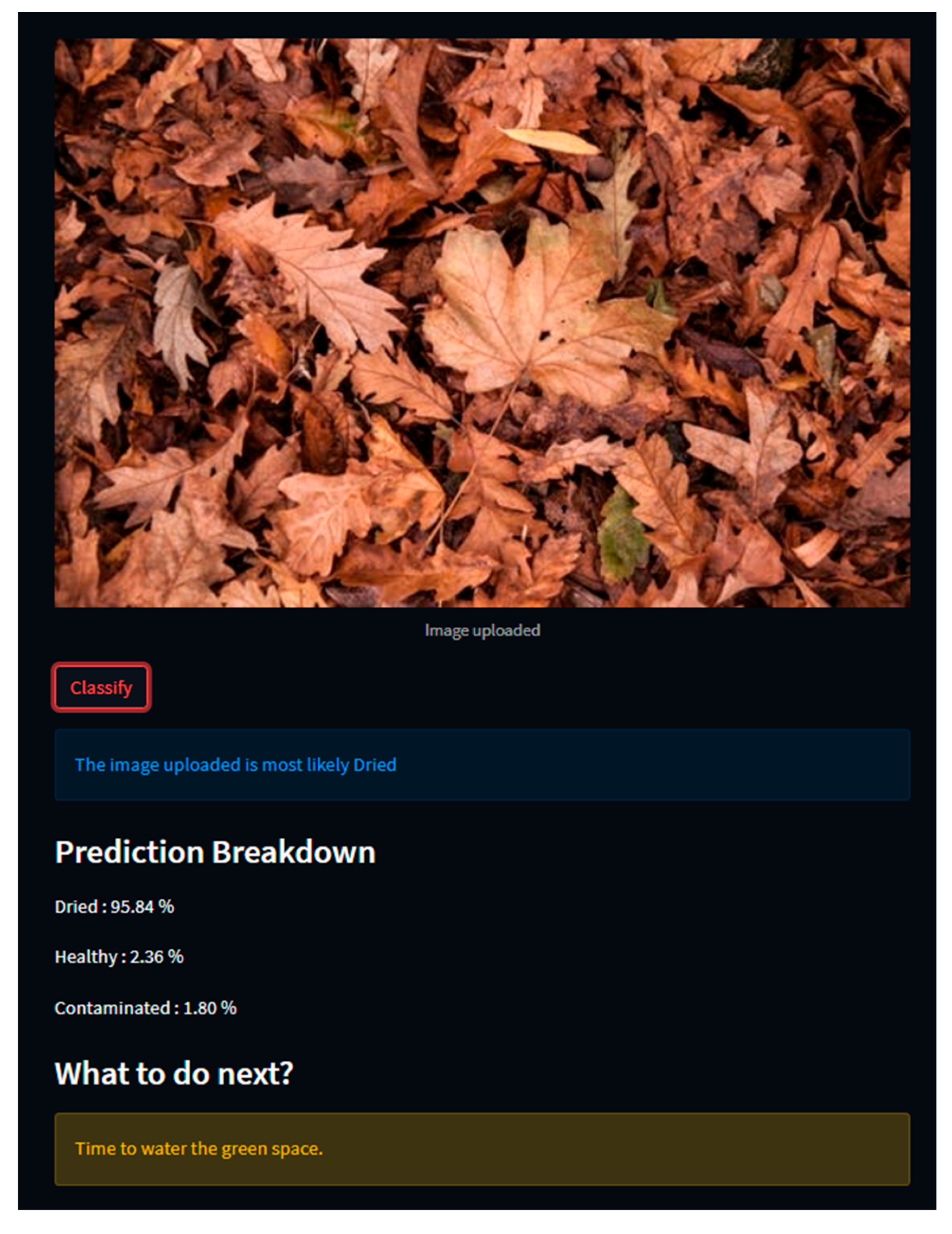
3.8. Deployment
3.9. Tools
4. Results and Discussion
4.1. Deployment
4.2. Challenges and Limitations
5. Conclusions
Author Contributions
Funding
Institutional Review Board Statement
Informed Consent Statement
Data Availability Statement
Acknowledgments
Conflicts of Interest
Appendix A

| Image Properties | Value |
|---|---|
| Dimensions | 3024 × 4032 pixels |
| Device Manufacturer & Model | Apple iPhone XR |
| Focal Length | 4.25 mm |
| F-Stop | f/1.8 |
| Exposure Time | 1/500 s |
| ISO | ISO 25 |
| Exposure Bias | 0 |
| Flash Status | No Flash |
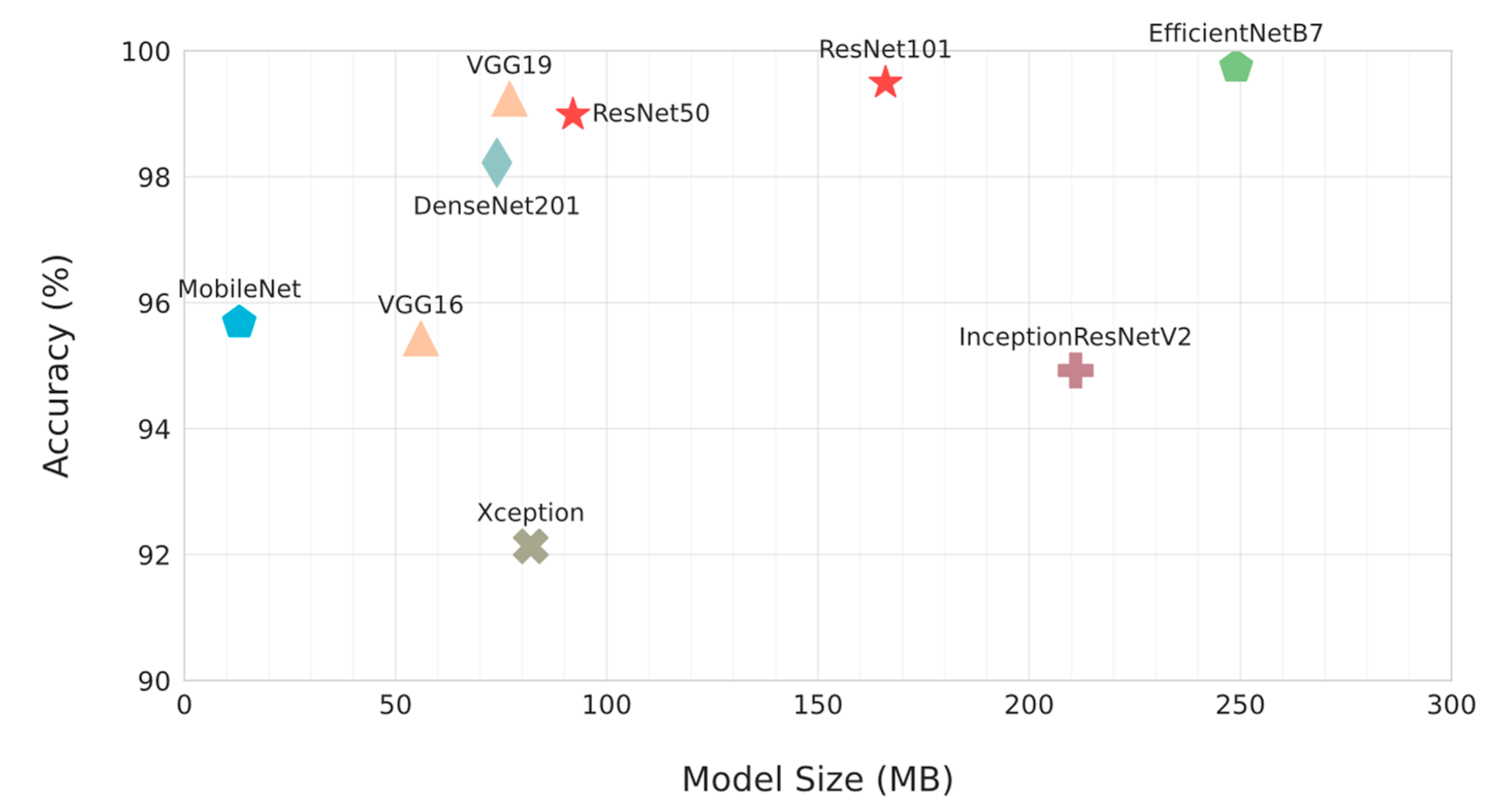
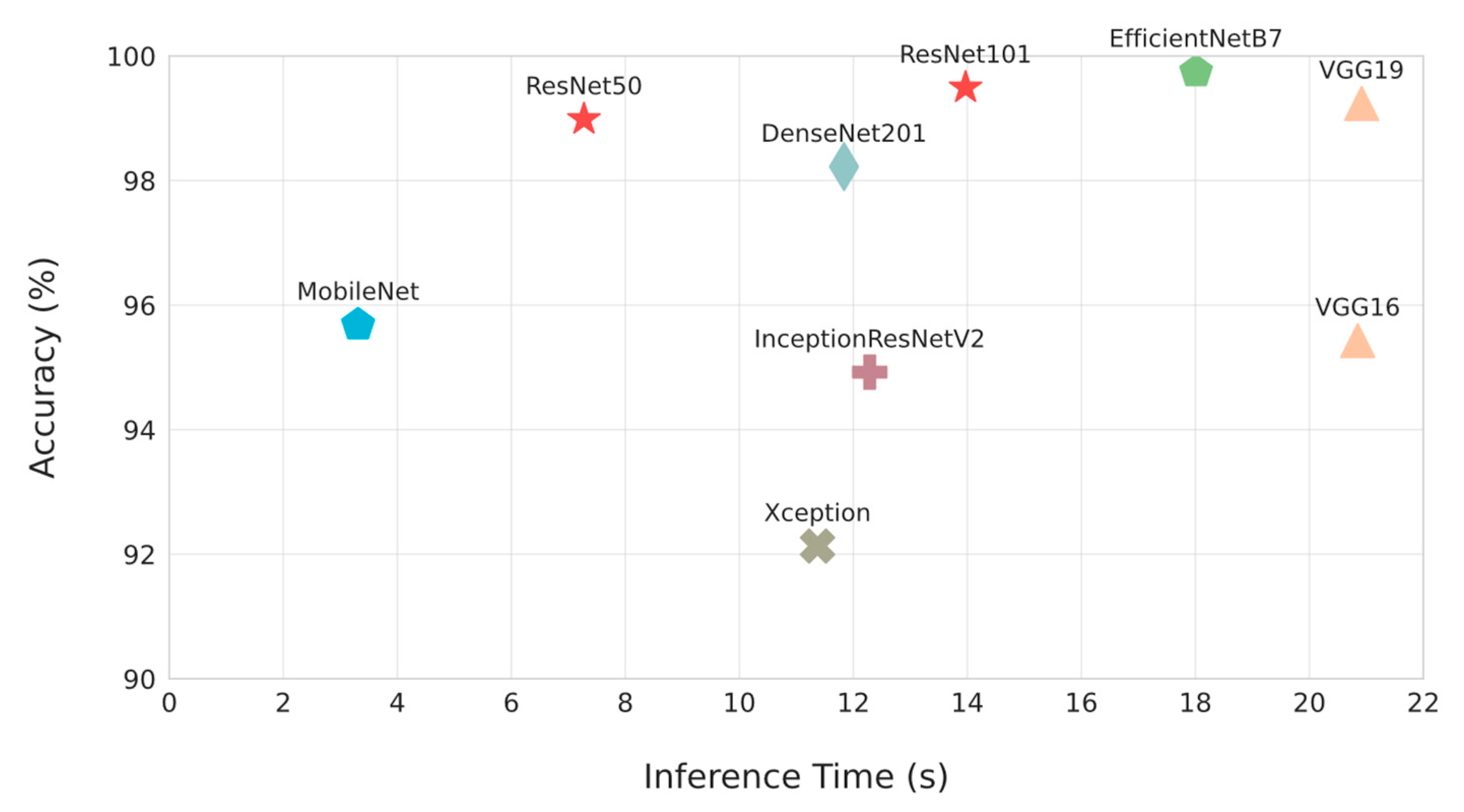
| Model | Avg. Inference Time (s) | File Size (MB) |
|---|---|---|
| DenseNet201 | 11.84 | 74 |
| EfficientNetB7 | 18.01 | 249 |
| InceptionResNetV2 | 12.29 | 211 |
| MobileNet | 3.31 | 13 |
| ResNet50 | 7.28 | 92 |
| ResNet101 | 13.97 | 166 |
| VGG-16 | 20.85 | 56 |
| VGG-19 | 20.92 | 77 |
| XCeption | 11.37 | 82 |
Appendix B


Appendix C


- Select an image from the device’s storage or capture an image using the device’s camera.
- Press the Classify button and wait for the result.
References
- Hoang, N.-D.; Tran, X.-L. Remote Sensing–Based Urban Green Space Detection Using Marine Predators Algorithm Optimized Machine Learning Approach. Math. Probl. Eng. 2021, 2021, 5586913. [Google Scholar] [CrossRef]
- Ki, D.; Lee, S. Analyzing the effects of Green View Index of neighborhood streets on walking time using Google Street View and deep learning. Landsc. Urban Plan. 2021, 205, 103920. [Google Scholar] [CrossRef]
- Knobel, P.; Dadvand, P.; Alonso, L.; Costa, L.; Español, M.; Maneja, R. Development of the urban green space quality assessment tool (RECITAL). Urban For. Urban Green. 2021, 57, 126895. [Google Scholar] [CrossRef]
- Meng, L.; Wen, K.-H.; Zeng, Z.; Brewin, R.; Fan, X.; Wu, Q. The Impact of Street Space Perception Factors on Elderly Health in High-Density Cities in Macau—Analysis Based on Street View Images and Deep Learning Technology. Sustainability 2020, 12, 1799. [Google Scholar] [CrossRef]
- Nguyen, P.-Y.; Astell-Burt, T.; Rahimi-Ardabili, H.; Feng, X. Green Space Quality and Health: A Systematic Review. Int. J. Environ. Res. Public Health 2021, 18, 11028. [Google Scholar] [CrossRef]
- Ord, K.; Mitchell, R.; Pearce, J. Is level of neighbourhood green space associated with physical activity in green space? Int. J. Behav. Nutr. Phys. Act. 2013, 10, 127. [Google Scholar] [CrossRef] [PubMed]
- Wang, W.; Lin, Z.; Zhang, L.; Yu, T.; Ciren, P.; Zhu, Y. Building visual green index: A measure of visual green spaces for urban building. Urban For. Urban Green 2019, 40, 335–343. [Google Scholar] [CrossRef]
- Xia, Y.; Yabuki, N.; Fukuda, T. Development of a system for assessing the quality of urban street-level greenery using street view images and deep learning. Urban For. Urban Green. 2021, 59, 126995. [Google Scholar] [CrossRef]
- Kothencz, G.; Kolcsár, R.; Cabrera-Barona, P.; Szilassi, P. Urban Green Space Perception and Its Contribution to Well-Being. Int. J. Environ. Res. Public Health 2017, 14, 766. [Google Scholar] [CrossRef]
- E van Dillen, S.M.; de Vries, S.; Groenewegen, P.P.; Spreeuwenberg, P. Greenspace in urban neighbourhoods and residents’ health: Adding quality to quantity. J. Epidemiol. Community Health 2012, 66, e8. [Google Scholar] [CrossRef]
- Hands, A.; Stimpson, A.; Ridgley, H.; Petrokofsky, C. Improving Access to Greenspace a New Review for 2020; Public Health England: Nottingham, UK, 2020. [Google Scholar] [CrossRef]
- Stessens, P.; Canters, F.; Huysmans, M.; Khan, A.Z. Urban green space qualities: An integrated approach towards GIS-based assessment reflecting user perception. Land Use Policy 2020, 91, 104319. [Google Scholar] [CrossRef]
- Bertram, C.; Rehdanz, K. Preferences for cultural urban ecosystem services: Comparing attitudes, perception, and use. Ecosyst. Serv. 2015, 12, 187–199. [Google Scholar] [CrossRef]
- Jim, C.Y.; Chen, W.Y. Recreation–amenity use and contingent valuation of urban greenspaces in Guangzhou, China. Landsc. Urban Plan. 2006, 75, 81–96. [Google Scholar] [CrossRef]
- Madureira, H.; Nunes, F.; Oliveira, J.V.; Madureira, T. Preferences for Urban Green Space Characteristics: A Comparative Study in Three Portuguese Cities. Environments 2018, 5, 23. [Google Scholar] [CrossRef]
- Qureshi, S.; Breuste, J.H.; Jim, C.Y. Differential community and the perception of urban green spaces and their contents in the megacity of Karachi, Pakistan. Urban Ecosyst. 2013, 16, 853–870. [Google Scholar] [CrossRef]
- Lee, H.-Y.; Tseng, H.-H.; Zheng, M.-C.; Li, P.-Y. Decision support for the maintenance management of green areas. Expert Syst. Appl. 2010, 37, 4479–4487. [Google Scholar] [CrossRef]
- Conservancy, C.P. Central Park Conservancy Annual Report 2021. 2021. Available online: https://assets.centralparknyc.org/media/documents/AnnualReport_Digital_2021_FinalREV1.pdf (accessed on 14 January 2023).
- Brynjolfsson, E.; Mitchell, T. Technology and the Economy|What Can Machine Learning Do? Workforce Implic. 2017, 358, 1530. [Google Scholar]
- Sun, Y.; Wang, X.; Zhu, J.; Chen, L.; Jia, Y.; Lawrence, J.M.; Jiang, L.-H.; Xie, X.; Wu, J. Using machine learning to examine street green space types at a high spatial resolution: Application in Los Angeles County on socioeconomic disparities in exposure. Sci. Total. Environ. 2021, 787, 147653. [Google Scholar] [CrossRef]
- Knobel, P.; Dadvand, P.; Maneja-Zaragoza, R. A systematic review of multi-dimensional quality assessment tools for urban green spaces. Health Place 2019, 59, 102198. [Google Scholar] [CrossRef]
- Moreno-Armendáriz, M.A.; Calvo, H.; Duchanoy, C.A.; López-Juárez, A.P.; Vargas-Monroy, I.A.; Suarez-Castañon, M.S. Deep Green Diagnostics: Urban Green Space Analysis Using Deep Learning and Drone Images. Sensors 2019, 19, 5287. [Google Scholar] [CrossRef]
- Wang, R.; Feng, Z.; Pearce, J.; Yao, Y.; Li, X.; Liu, Y. The distribution of greenspace quantity and quality and their association with neighbourhood socioeconomic conditions in Guangzhou, China: A new approach using deep learning method and street view images. Sustain. Cities Soc. 2021, 66, 102664. [Google Scholar] [CrossRef]
- Dadvand, P.; Nieuwenhuijsen, M. Green Space and Health; Springer International Publishing: Cham, Switzerland, 2019; pp. 409–423. [Google Scholar] [CrossRef]
- Swanwick, C.; Dunnett, N.; Woolley, H. Nature, Role and Value of Green Space in Towns and Cities: An Overview. Built Environ. 2003, 29, 94–106. [Google Scholar] [CrossRef]
- Qiu, Y.; Zuo, S.; Yu, Z.; Zhan, Y.; Ren, Y. Discovering the effects of integrated green space air regulation on human health: A bibliometric and meta-analysis. Ecol. Indic. 2021, 132, 108292. [Google Scholar] [CrossRef]
- Bertram, C.; Rehdanz, K. The role of urban green space for human well-being. Ecol. Econ. 2015, 120, 139–152. [Google Scholar] [CrossRef]
- Holt, E.W.; Lombard, Q.K.; Best, N.; Smiley-Smith, S.; Quinn, J.E. Active and Passive Use of Green Space, Health, and Well-Being amongst University Students. Int. J. Environ. Res. Public Health 2019, 16, 424. [Google Scholar] [CrossRef]
- Kabisch, N.; Qureshi, S.; Haase, D. Human–environment interactions in urban green spaces—A systematic review of contemporary issues and prospects for future research. Environ. Impact Assess. Rev. 2015, 50, 25–34. [Google Scholar] [CrossRef]
- Jennings, V.; Bamkole, O. The Relationship between Social Cohesion and Urban Green Space: An Avenue for Health Promotion. Int. J. Environ. Res. Public Health 2019, 16, 452. [Google Scholar] [CrossRef]
- Perković, D.; Opačić, V.T. Methodological approaches in research on urban green spaces in the context of coastal tourism development. Geoadria 2020, 25, 53–89. [Google Scholar] [CrossRef]
- Lal, R. Carbon sequestration. Philos. Trans. R. Soc. B Biol. Sci. 2008, 363, 815–830. [Google Scholar] [CrossRef]
- Bowler, D.E.; Buyung-Ali, L.; Knight, T.M.; Pullin, A.S. Urban greening to cool towns and cities: A systematic review of the empirical evidence. Landsc. Urban Plan. 2010, 97, 147–155. [Google Scholar] [CrossRef]
- Akpinar, A. How is quality of urban green spaces associated with physical activity and health? Urban For. Urban Green. 2016, 16, 76–83. [Google Scholar] [CrossRef]
- Colesca, S.E.; Alpopi, C. The quality of bucharest’s green spaces. Theor. Empir. Res. Urban Manag. 2011, 6, 45–59. Available online: http://www.jstor.org/stable/24873301 (accessed on 25 January 2023).
- Zhang, Y.; Van den Berg, A.E.; Van Dijk, T.; Weitkamp, G. Quality over Quantity: Contribution of Urban Green Space to Neighborhood Satisfaction. Int. J. Environ. Res. Public Health 2017, 14, 535. [Google Scholar] [CrossRef]
- Lu, Y. Using Google Street View to investigate the association between street greenery and physical activity. Landsc. Urban Plan. 2019, 191, 103435. [Google Scholar] [CrossRef]
- Gidlow, C.J.; Ellis, N.J.; Bostock, S. Development of the Neighbourhood Green Space Tool (NGST). Landsc. Urban Plan. 2012, 106, 347–358. [Google Scholar] [CrossRef]
- Hillsdon, M.; Panter, J.; Foster, C.; Jones, A. The relationship between access and quality of urban green space with population physical activity. Public Health 2006, 120, 1127–1132. [Google Scholar] [CrossRef] [PubMed]
- Putra, I.G.N.E.; Astell-Burt, T.; Cliff, D.P.; Vella, S.A.; Feng, X. Association between green space quality and prosocial behaviour: A 10-year multilevel longitudinal analysis of Australian children. Environ. Res. 2021, 196, 110334. [Google Scholar] [CrossRef]
- Chen, B.; Adimo, O.A.; Bao, Z. Assessment of aesthetic quality and multiple functions of urban green space from the users’ perspective: The case of Hangzhou Flower Garden, China. Landsc. Urban Plan. 2009, 93, 76–82. [Google Scholar] [CrossRef]
- Helbich, M.; Yao, Y.; Liu, Y.; Zhang, J.; Liu, P.; Wang, R. Using deep learning to examine street view green and blue spaces and their associations with geriatric depression in Beijing, China. Environ. Int. 2019, 126, 107–117. [Google Scholar] [CrossRef]
- Ta, D.T.; Furuya, K. Google Street View and Machine Learning—Useful Tools for a Street-Level Remote Survey: A Case Study in Ho Chi Minh, Vietnam and Ichikawa, Japan. Land 2022, 11, 2254. [Google Scholar] [CrossRef]
- Phan, C.; Raheja, A.; Bhandari, S.; Green, R.L.; Do, D. A predictive model for turfgrass color and quality evaluation using deep learning and UAV imageries. SPIE 2017, 10218, 102180. [Google Scholar] [CrossRef]
- Larkin, A.; Krishna, A.; Chen, L.; Amram, O.; Avery, A.R.; Duncan, G.E.; Hystad, P. Measuring and modelling perceptions of the built environment for epidemiological research using crowd-sourcing and image-based deep learning models. J. Expo. Sci. Environ. Epidemiol. 2022, 32, 892–899. [Google Scholar] [CrossRef]
- Ghahramani, M.; Galle, N.J.; Duarte, F.; Ratti, C.; Pilla, F. Leveraging artificial intelligence to analyze citizens’ opinions on urban green space. City Environ. Interact. 2021, 10, 100058. [Google Scholar] [CrossRef]
- Ye, Y.; Richards, D.; Lu, Y.; Song, X.; Zhuang, Y.; Zeng, W.; Zhong, T. Measuring daily accessed street greenery: A human-scale approach for informing better urban planning practices. Landsc. Urban Plan. 2019, 191, 103434. [Google Scholar] [CrossRef]
- Bosnjak, Z.; Grljevic, O. CRISP-DM as a framework for discovering knowledge in small and medium sized enterprises’ data. In Proceedings of the 2009 5th International Symposium on Applied Computational Intelligence and Informatics, Timisoara, Romania, 28–29 May 2009; pp. 509–514. [Google Scholar] [CrossRef]
- Jaggia, S.; Kelly, A.; Lertwachara, K.; Chen, L. Applying the CRISP-DM Framework for Teaching Business Analytics. Decis. Sci. J. Innov. Educ. 2020, 18, 612–634. [Google Scholar] [CrossRef]
- Wirth, R.; Hipp, J. CRISP-DM: Towards a standard process model for data mining. In Proceedings of the Fourth International Conference on the Practical Application of Knowledge Discovery and Data Mining, Manchester, UK, 11–13 April 2000; pp. 29–39. Available online: https://www.researchgate.net/publication/239585378_CRISP-DM_Towards_a_standard_process_model_for_data_mining (accessed on 2 January 2023).
- Li, Z.; Kamnitsas, K.; Glocker, B. Analyzing Overfitting Under Class Imbalance in Neural Networks for Image Segmentation. IEEE Trans. Med. Imaging 2021, 40, 1065–1077. [Google Scholar] [CrossRef] [PubMed]
- Ferreira, C.A.; Melo, T.; Sousa, P.; Meyer, M.I.; Shakibapour, E.; Costa, P.; Campilho, A. Classification of Breast Cancer Histology Images Through Transfer Learning Using a Pre-trained Inception Resnet V2. In Image Analysis and Recognition, Proceedings of the 15th International Conference, ICIAR 2018, Póvoa de Varzim, Portugal, 27–29 June 2018; Springer International Publishing: Berlin/Heidelberg, Germany, 2018; pp. 763–770. [Google Scholar] [CrossRef]
- Yadav, G.; Maheshwari, S.; Agarwal, A. Contrast limited adaptive histogram equalization based enhancement for real time video system. In Proceedings of the 2014 International Conference on Advances in Computing, Communications and Informatics (ICACCI), Delhi, India, 24–27 September 2014; pp. 2392–2397. [Google Scholar] [CrossRef]
- Wong, L.J.; Michaels, A.J. Transfer Learning for Radio Frequency Machine Learning: A Taxonomy and Survey. Sensors 2022, 22, 1416. [Google Scholar] [CrossRef]
- Ayadi, S.; Lachiri, Z. Deep Neural Network for visual Emotion Recognition based on ResNet50 using Song-Speech characteristics. In Proceedings of the 2022 5th International Conference on Advanced Systems and Emergent Technologies (IC_ASET), Hammamet, Tunisia, 22–25 March 2022; pp. 363–368. [Google Scholar] [CrossRef]
- Jibhakate, A.; Parnerkar, P.; Mondal, S.; Bharambe, V.; Mantri, S. Skin Lesion Classification using Deep Learning and Image Processing. In Proceedings of the 2020 3rd International Conference on Intelligent Sustainable Systems (ICISS), Thoothukudi, India, 3–5 December 2020; pp. 333–340. [Google Scholar] [CrossRef]
- Raihan, M.; Suryanegara, M. Classification of COVID-19 Patients Using Deep Learning Architecture of InceptionV3 and ResNet50. In Proceedings of the 2021 4th International Conference of Computer and Informatics Engineering (IC2IE), Depok, Indonesia, 14–15 September 2021; pp. 46–50. [Google Scholar] [CrossRef]
- Tian, X.; Chen, C. Modulation Pattern Recognition Based on Resnet50 Neural Network. In Proceedings of the Modulation Pattern Recognition Based on Resnet50 Neural Network, Weihai, China, 28–30 September 2019; pp. 34–38. [Google Scholar] [CrossRef]
- Singh, P.; Verma, A.; Alex, J.S.R. Disease and pest infection detection in coconut tree through deep learning techniques. Comput. Electron. Agric. 2021, 182, 105986. [Google Scholar] [CrossRef]
- Mascarenhas, S.; Agarwal, M. A comparison between VGG16, VGG19 and ResNet50 architecture frameworks for Image Classification. In Proceedings of the 2021 International Conference on Disruptive Technologies for Multi-Disciplinary Research and Applications (CENTCON), Bengaluru, India, 19–21 November 2021; Volume 1, pp. 96–99. [Google Scholar] [CrossRef]
- Khade, S.; Gite, S.; Pradhan, B. Iris Liveness Detection Using Multiple Deep Convolution Networks. Big Data Cogn. Comput. 2022, 6, 67. [Google Scholar] [CrossRef]
- Gupta, R.K.; Kunhare, N.; Pathik, N.; Pathik, B. An AI-enabled pre-trained model-based Covid detection model using chest X-ray images. Multimed. Tools Appl. 2022, 81, 37351–37377. [Google Scholar] [CrossRef]
- Sutaji, D.; Yıldız, O. LEMOXINET: Lite ensemble MobileNetV2 and Xception models to predict plant disease. Ecol. Inform. 2022, 70, 101698. [Google Scholar] [CrossRef]
- Lo, W.W.; Yang, X.; Wang, Y. An Xception Convolutional Neural Network for Malware Classification with Transfer Learning. In Proceedings of the 2019 10th IFIP International Conference on New Technologies, Mobility and Security (NTMS), Canary Islands, Spain, 24–26 June 2019; pp. 1–5. [Google Scholar] [CrossRef]
- Jethwa, N.; Gabajiwala, H.; Mishra, A.; Joshi, P.; Natu, P. Comparative Analysis between InceptionResnetV2 and InceptionV3 for Attention based Image Captioning. In Proceedings of the 2021 2nd Global Conference for Advancement in Technology (GCAT), Bangalore, India, 1–3 October 2021; pp. 1–6. [Google Scholar] [CrossRef]
- Thomas, A.; Harikrishnan, P.M.; Palanisamy, P.; Gopi, V.P. Moving Vehicle Candidate Recognition and Classification Using Inception-ResNet-v2. In Proceedings of the 2020 IEEE 44th Annual Computers, Software, and Applications Conference (COMPSAC), Madrid, Spain, 13–17 July 2020; pp. 467–472. [Google Scholar] [CrossRef]
- Aslam, N.; Khan, I.U.; Albahussain, T.I.; Almousa, N.F.; Alolayan, M.O.; Almousa, S.A.; Alwhebi, M.E. MEDeep: A Deep Learning Based Model for Memotion Analysis. Math. Model. Eng. Probl. 2022, 9, 533–538. [Google Scholar] [CrossRef]
- Delgado, R.; Tibau, X.-A. Why Cohen’s Kappa should be avoided as performance measure in classification. PLoS ONE 2019, 14, e0222916. [Google Scholar] [CrossRef] [PubMed]
- Salminen, J.; Kandpal, C.; Kamel, A.M.; Jung, S.-G.; Jansen, B.J. Creating and detecting fake reviews of online products. J. Retail. Consum. Serv. 2022, 64, 102771. [Google Scholar] [CrossRef]
- Nafisah, S.I.; Muhammad, G. Tuberculosis detection in chest radiograph using convolutional neural network architecture and explainable artificial intelligence. Neural Comput. Appl. 2022, 6. [Google Scholar] [CrossRef]
- Lee, C.; Lin, J.; Prokop, A.; Gopalakrishnan, V.; Hanna, R.N.; Papa, E.; Freeman, A.; Patel, S.; Yu, W.; Huhn, M.; et al. StarGazer: A Hybrid Intelligence Platform for Drug Target Prioritization and Digital Drug Repositioning Using Streamlit. Front. Genet. 2022, 13, 868015. [Google Scholar] [CrossRef]
- Sun, D.; Xu, Y.; Shen, M. Efficient Models Selecting, 2018. Available online: https://digital.wpi.edu/concern/student_works/73666612z (accessed on 2 January 2023).
- Simonyan, K.; Zisserman, A. Very deep convolutional networks for large-scale image recognition. arXiv 2014, arXiv:1409.1556. [Google Scholar] [CrossRef]
- He, K.; Zhang, X.; Ren, S.; Sun, J. Deep residual learning for image recognition. In Proceedings of the IEEE Computer Society Conference on Computer Vision and Pattern Recognition (CVPR), Las Vegas, NV, USA, 27–30 June 2016; pp. 770–778. [Google Scholar] [CrossRef]
- Zhang, Z.; Sabuncu, M. Generalized cross entropy loss for training deep neural networks with noisy labels. Adv. Neural Inf. Process. Syst. 2018, 31, 8778–8788. [Google Scholar]
- Sandler, M.; Howard, A.; Zhu, M.; Zhmoginov, A.; Chen, L. MobileNetV2: Inverted residuals and linear bottlenecks. In Proceedings of the IEEE/CVF Conference on Computer Vision and Pattern Recognition (CVPR), Salt Lake City, UT, USA, 18–23 June 2018; pp. 4510–4520. [Google Scholar] [CrossRef]
- Howard, A.G.; Zhu, M.; Chen, B.; Kalenichenko, D.; Wang, W.; Weyand, T.; Andreetto, M.; Adam, H. MobileNets: Efficient Convolutional Neural Networks for Mobile Vision Applications. arXiv 2017, arXiv:1704.04861. [Google Scholar]


| Paper | Green Space Type | Quality Factors Assessed | Method of Assessment |
|---|---|---|---|
| [41] | Bonsais and flowers | Aesthetic quality | Quantitative holistic technique |
| [39] | Green space | Accessibility, maintenance, recreational facilities, amenity provision, signage and lighting, landscape, usage, and atmosphere. | Regression models |
| [12] | Green space, public areas | Nature and biodiversity, quietness, historical and cultural value, spaciousness, facilities, cleanliness and maintenance, safety. | Perception of green space users |
| [3] | Municipality and urban areas | Surroundings, access, facilities, amenities, aesthetics and attractions, incivilities, potential usage, land covers, animal biodiversity and birds’ biodiversity. | Five-point Likert scale |
| [36] | Neighborhood | Recreation facilities, amenities for a picnic, natural features, absence of incivilities, accessibility, maintenance. | Statistical analyses |
| [38] | Neighborhood | Appearance, maintenance, and the presence of quality of various features | - |
| [35] | Park | Green space placement, green space use, environment, biodiversity | Five-point Likert scale |
| [40] | Park, playground | Availability | Likert scale |
| [34] | Park, urban greenway | Distance to green space, aesthetic, cleanliness, largeness, maintenance, shaded areas, lights, openness/visibility | Series of multivariate linear regression analyses |
| [37] | Street | Greenery, absence of litter, maintenance, general condition | Five-point Likert scale |
| Paper | Green Space Type | Quality Factors Assessed | ML Model | Results |
|---|---|---|---|---|
| [45] | Forest, park, cityscape | - | DeepLabV3+ | Accuracy: 65% |
| [2] | Park | - | SVM | AUC: 97.2%, precision: 97.1%, recall: 99.7%, F1-score: 98.3% |
| [8] | Park, garden | Visibility of greenery | DeepLabV3+ | mIoU: 78.37%, RMSE: 2.75%, MAE: 2.28% |
| [23] | Street | Accessibility, maintenance, variation, naturalness, colorfulness, clear arrangement, shelter, absence of litter, safety, general impression | Random Forest | Pearson’s correlation coefficient: 0.90 |
| [42] | Street | Pedestrian and commuting accessibility, street greenery | SVM | Cohen’s Kappa coefficient: 0.925 |
| [43] | Street | Visibility of greenery | FCN-8s | Accuracy: 84.56% |
| [44] | Street | - | FCN-8s | Accuracy: 76.8% |
| [47] | Street | Nature quality, beauty, relaxation, safety | CNN | Accuracy: 70.53% |
| [22] | Terrain | Health, contamination | Deep Neural Network | Accuracy: 72%, precision: 72%, recall: 72%, F1-score: 71% |
| [46] | Turfgrass | Hue, texture, color, leaf blade width, uniformity | Inception-V3 | Accuracy: 73.35%, loss: 40.25% |
| Phase | Description |
|---|---|
| Business Understanding | The project objectives and requirements are defined in this stage, and a preliminary plan is developed to address the business problem. This stage involves understanding the goals and objectives of the project and how the data mining solution will be used to solve the business problem. |
| Data Understanding | In this stage, data sources are identified, and data is collected, explored, and described. This stage involves getting familiar with the available data, its quality, and its limitations, and identifying any data issues that need to be addressed. |
| Data Preparation | Data is cleansed, transformed, and pre-processed in this stage to prepare for modeling. This stage involves selecting the relevant data, creating new variables, handling missing values, and addressing other data quality issues. |
| Modelling | In this stage, various modeling techniques are applied to the prepared data. This stage involves selecting and applying appropriate modeling techniques, evaluating model performance, and selecting the best model. |
| Evaluation | In this stage, the model is evaluated to determine whether it meets the business objectives. This stage involves assessing the model’s performance, comparing it to other models, and assessing its generalizability and applicability. |
| Deployment | In this stage, the model is deployed into a production environment. This stage involves implementing the model, monitoring its performance, and making necessary adjustments. |
| Transformation Technique | Parameter | Description |
|---|---|---|
| HorizontalFlip | p = 0.5 | Flips the supplied image horizontally. |
| RandomBrightnessContrast | p = 0.5 | Randomly alters the brightness and contrast of the image supplied. |
| RandomRotate90 | p = 0.5 | Randomly rotates the image supplied by 90 degrees zero or more times. |
| CLAHE | p = 0.5 | Applies Contrast Limited Adaptive Histogram Equalisation (CLAHE) to the image, enhancing an image’s or video’s visibility level [52]. |
| Dataset Features | Value |
|---|---|
| Total observations | 986 |
| Total training data | 710 |
| Total validation data | 78 |
| Total testing data | 197 |
| Number of classes | 3 |
| Parameter | Value |
|---|---|
| Data split | Training: 70%, Testing: 20%, Validation Split: 10% |
| Image size | 224 × 224 × 3 |
| Weight | ImageNet |
| Epochs | 50 |
| Batch size | 32 |
| Optimization algorithm | Adam (learning rate: 0.001) |
| Regularization algorithm | ReduceLROnPlateau (patience: 2, factor: 0.1), Early Stopping (patience: 4) |
| Loss function | Categorical Cross-entropy |
| Model | Depth (no. of Layers) | Time Taken to Predict (ms) | Model File Size | Skip Connections | Architectural Complexity |
|---|---|---|---|---|---|
| MobileNet | 27 | 1–2 | Small | Yes | Simple |
| XCeption | 71 | 3–4 | Small | Yes | Simple |
| DenseNet201 | 201 | 10–11 | Small | Yes | Complex |
| ResNet50 | 50 | 2–3 | Medium | Yes | Simple |
| ResNet101 | 101 | 7–8 | Medium | Yes | Complex |
| InceptionResNetV2 | 164 | 8–9 | Medium | Yes | Complex |
| VGG-16 | 16 | 5–6 | Large | No | Simple |
| VGG-19 | 19 | 6–7 | Large | No | Simple |
| EfficientNetB7 | 813 | 25–30 | Large | Yes | Complex |
| Component | Brand and Model |
|---|---|
| Operating System (OS) | Windows 10 Professional Edition (Version 21H2, Build 19044.1826) |
| Central Processing Unit (CPU) | AMD Ryzen 7 5800X |
| Graphical Processing Unit (GPU) | Nvidia GTX 1080 Ti 11GB GDDR5 |
| Random Access Memory (RAM) | 32GB @ 3800 MHz |
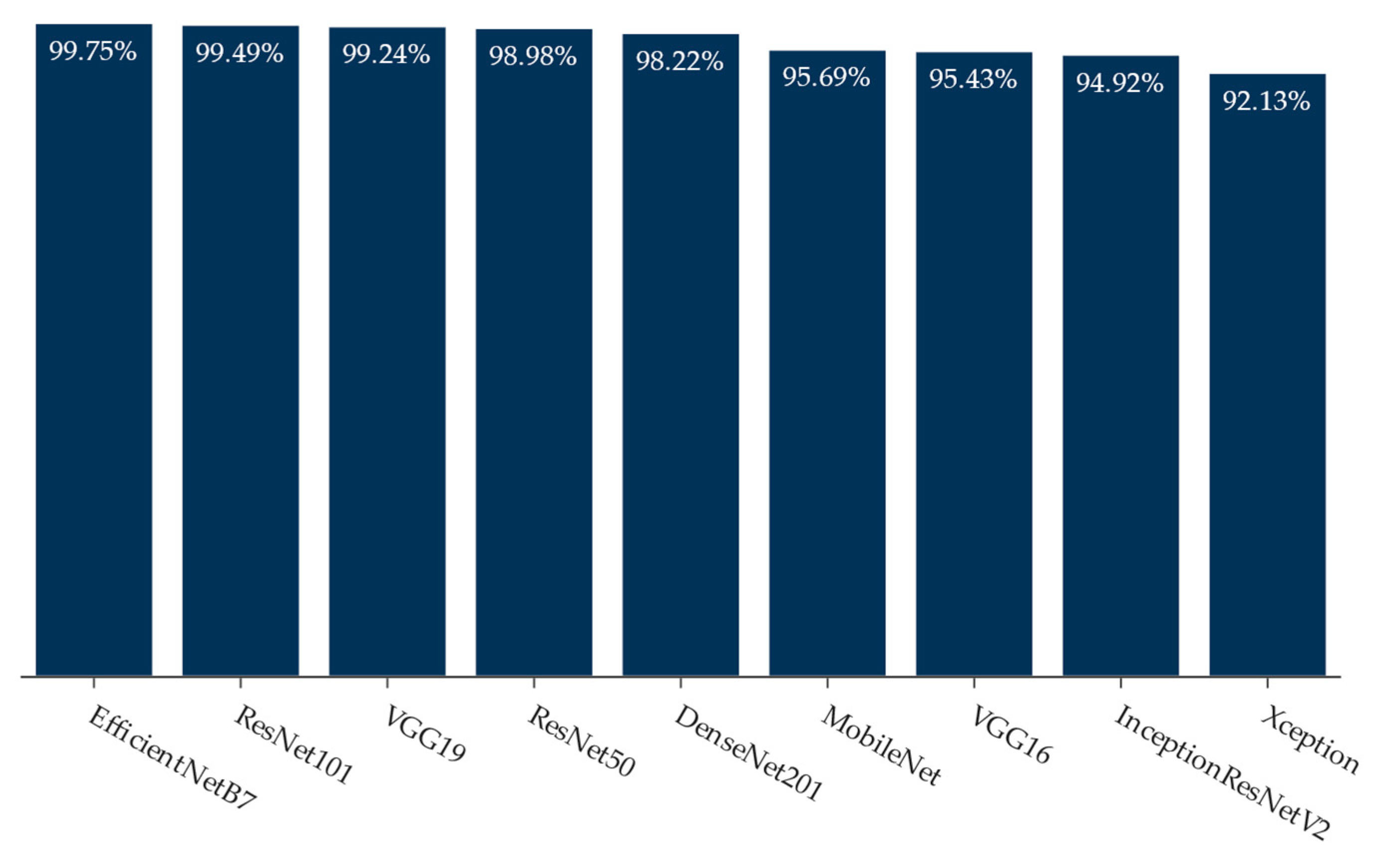
| Model | Accuracy (%) | Precision (%) | Recall (%) | F1-Score (%) | Kappa | ROC-AUC |
|---|---|---|---|---|---|---|
| XCeption | 92.13 | 92.13 | 92.13 | 92.12 | 0.88 | 0.98 |
| InceptionResNetV2 | 94.92 | 94.96 | 94.92 | 94.93 | 0.92 | 1.00 |
| VGG-16 | 95.43 | 95.43 | 95.43 | 95.43 | 0.93 | 0.99 |
| MobileNet | 95.69 | 95.81 | 95.69 | 95.70 | 0.94 | 0.99 |
| DenseNet201 | 98.22 | 98.24 | 98.22 | 98.23 | 0.97 | 1.00 |
| ResNet50 | 98.98 | 99.00 | 98.98 | 98.98 | 0.98 | 1.00 |
| ResNet101 | 99.49 | 99.49 | 99.49 | 99.49 | 0.99 | 1.00 |
| VGG-19 | 99.24 | 99.24 | 99.24 | 99.24 | 0.99 | 1.00 |
| EfficientNetB7 | 99.75 | 99.75 | 99.75 | 99.75 | 1.00 | 1.00 |
Disclaimer/Publisher’s Note: The statements, opinions and data contained in all publications are solely those of the individual author(s) and contributor(s) and not of MDPI and/or the editor(s). MDPI and/or the editor(s) disclaim responsibility for any injury to people or property resulting from any ideas, methods, instructions or products referred to in the content. |
© 2023 by the authors. Licensee MDPI, Basel, Switzerland. This article is an open access article distributed under the terms and conditions of the Creative Commons Attribution (CC BY) license (https://creativecommons.org/licenses/by/4.0/).
Share and Cite
Rustamov, J.; Rustamov, Z.; Zaki, N. Green Space Quality Analysis Using Machine Learning Approaches. Sustainability 2023, 15, 7782. https://doi.org/10.3390/su15107782
Rustamov J, Rustamov Z, Zaki N. Green Space Quality Analysis Using Machine Learning Approaches. Sustainability. 2023; 15(10):7782. https://doi.org/10.3390/su15107782
Chicago/Turabian StyleRustamov, Jaloliddin, Zahiriddin Rustamov, and Nazar Zaki. 2023. "Green Space Quality Analysis Using Machine Learning Approaches" Sustainability 15, no. 10: 7782. https://doi.org/10.3390/su15107782
APA StyleRustamov, J., Rustamov, Z., & Zaki, N. (2023). Green Space Quality Analysis Using Machine Learning Approaches. Sustainability, 15(10), 7782. https://doi.org/10.3390/su15107782