Abstract
In order to satisfy increasing energy demand and mitigate global warming worldwide, the implementation of photovoltaic (PV) clean energy installations needs to become common practice. However, solar energy is known to be dependent on several random factors, including climatic and geographic conditions. Prior to promoting PV systems, an assessment study of the potential of the considered location in terms of power yield should be conducted carefully. Manual assessment tools are unable to handle high amounts of data. In order to overcome this difficulty, this study aims to investigate various artificial intelligence (AI) models—with respect to various intuitive prediction benchmark models from the literature—for predicting solar energy yield in the Ha’il region of Saudi Arabia. Based on the daily data, seven seasonal models, namely, naïve (N), simple average (SA), simple moving average (SMA), nonlinear auto-regressive (NAR), support vector machine (SVM), Gaussian process regression (GPR) and neural network (NN), were investigated and compared based on the root mean square error (RMSE) and mean absolute percentage error (MAPE) performance metrics. The obtained results showed that all the models provided good forecasts over three years (2019, 2020, and 2021), with the naïve and simple moving average models showing small superiority. The results of this study can be used by decision-makers and solar energy specialists to analyze the power yield of solar systems and estimate the payback and efficiency of PV projects.
1. Introduction
Energy needs are constantly increasing worldwide due to intense industrial activities as well as population growth. Meanwhile, fossil fuel energy resources are extremely harmful to the environment and human health because of carbon dioxide emissions and global warming, inducing climate changes [1]. In order to overcome these issues and guarantee sufficient amounts of power, a new trend that appeared a few years ago is the massive investment in renewable clean energy, including wind and photovoltaic solar. The latter is expected to contribute 11% to global electricity consumption by the year 2050 [2]. However, the integration of solar energy with the currently existing grids may cause several problems, such as grid instability due to solar power’s intermittent and variable nature. In fact, solar energy is known to depend on several factors, including climatic conditions, which are completely uncontrollable [3]. Before any new investment in a solar energy project, the current and future potential of this source should be assessed carefully, taking into account the expected site parameters. Solar energy measurement devices are not available at every location. In addition, their accuracy remains questionable since they require frequent maintenance and calibration. In order to overcome these difficulties, solar energy practitioners resorted to assessing the current solar energy resources and forecasting future amounts using various techniques [4]. Solar radiation forecasting models can be mainly categorized into two families: empirical models [5,6] and machine learning (ML) models.
Based on a dataset collected from Najran University (Saudi Arabia) for the years 2017–2018, the author of [7] has investigated several machine and deep learning models, including a convolutional neural network (CNN) and a support vector machine (SVM) for predicting the daily global horizontal irradiation (GHI), as explained by climatic variables. The results were found to be satisfactory, with small merit given to the support vector classifier (SVC). SVCs also attracted the researchers of [8] to analyze and monitor a 270 Wp solar installation in Algeria. The authors assessed the performance of this station after seven months of operation/monitoring and found it continues functioning efficiently and that its original technical features remain consistent.
From an application perspective, the use of ML in solar power yield forecasting has also attracted the interest of researchers. One study [9] was dedicated to the prediction of output power from a small-scale residential system in Abha, Saudi Arabia, and another study [10] was allocated to an industrial experience conducted in Russia.
The prediction horizon was also an important factor in forecasting solar energy applications. For example, the very-short term horizon (10 min) [11], which may be used for efficient operation and control, and the short-term (daily) horizon [12], used for modeling the effect of pollution indicators on global and diffuse solar energy, as well as multistep ahead forecasting horizon [13].
Because temperature is the easiest climatic variable that can be measured, empirical models (commonly called temperature-based) based on temperature have been investigated for assessing the amount of solar energy power yielded at a given location [14,15]. These models have been shown to allow for spatial-temporal assessment with respectful accuracy.
The authors of [16] compared the performance of empirical and artificial neural networks (ANNs) in predicting daily solar radiation over 20 stations in Iran. An ANN coupled with a genetic algorithm (GA), referred to as ANN-GA, was found to outperform the other models, although they can be considered quite accurate.
The work conducted in [17] focused on finding the optimal structure of multilayer perceptrons (MLPs), recurrent neural networks (RNNs), and CNNs via the help of hybrid optimization algorithms, such as wolf optimization (WO), which were used to optimally tune the structure of the artificial intelligence (AI) techniques investigated. In fact, finding such optimal structures is known to be problematic since this was usually conducted based on a trial-and-error method that was reported to be time-consuming.
Several ML techniques have been utilized to forecast the hourly power yielded by a photovoltaic installation under the climatic conditions in Rabat, Morocco. Bayesian regularized neural networks (BRNNs) have been found to outperform other ML techniques, such as random forest (RF) and support vector regression (SVR). A principal component analysis (PCA) procedure was used to select the most meaningful climatic parameters [18].
The hybridization of ML techniques with population-based optimization techniques has been tested in several papers, including [19,20], where a back-propagation NN was combined with particle swarm optimization (BP-PSO) and an artificial neural network that was hybridized with differential evolution (ANN-DE), respectively. Hybridization has been shown to be an efficient solution to increase the accuracy and reliability of forecasts.
In order to study the discrepancy in the forecasting results when using ML, several other studies have been conducted in different locations and under different conditions. Among those studies, the following can be shown to cite a few: data-driven methods for Queensland, Australia [21], publicly available data for Germany [22], and weather and location data in the USA [23].
Based on references [7,8,9,10,11,12,13,14,15,16,17,18,19,20,21,22,23], the research limitations faced when using AI techniques to forecast PV power installation yields can be summarized as follows. First, all the developed techniques required the use of trial-and-error procedures to identify the model’s parameters, which is known to be time-consuming. Until now, and to the best knowledge of the authors’ knowledge, there is no systematic procedure to set up such parameters. Second, AI techniques (particularly DL) are known to require high amounts of data which are not usually available, particularly for short-term horizons. Finally, clear sky issues represent the key parameters for predicting solar radiation. The majority of studies did not consider intermittent skies, which may affect the PV power yield. The unique studies that provided high accuracy were conducted in locations with a clear sky day percentage that was high over a year.
The main contributions of the current study can be summarized as follows:
- -
- To the best of the authors’ knowledge, this study is among only a few works that have assessed various state-of-the-art ML approaches for predicting solar energy yield in a desert climate (the Ha’il region, Saudi Arabia), with respect to various simple and intuitive prediction approaches. Through the conducted comparative study, the main features that may affect solar power yield in the considered location have been identified, and the best models that provided the best forecasts have been investigated;
- -
- Such a contribution will pave the way for promoting PV systems in a considered location potential in terms of power yield, which may allow for the assessment of the efficiency of solar projects prior to field implementation;
- -
- The results of the present study are of high importance for evaluating the contribution of PV solar systems to environmental sustainability and the fight against climate change.
The rest of the paper is organized as follows: materials and methods are provided in Section 2, including the dataset used in this study and the prediction methodology proposed in this work. Section 3 illustrates the obtained results with a deep discussion and comparative analysis. Finally, our conclusions and perspectives are presented in Section 4.
2. Materials and Methods
2.1. Dataset
The dataset collected in this work from the NASA repository (i.e., NASA/POWER CERES/MERRA2 Native Resolution Daily Data: https://power.larc.nasa.gov/data-access-viewer/(accessed on 23 September 2022)) comprises 21 parameters for which the physical meaning, abbreviations, and units are reported in Table 1.

Table 1.
Dataset description.
The first three parameters represent the chronological order (i.e., timestamps) of the collected data, i.e., year, month, and day counters, respectively. The following 17 parameters represent the predictors (i.e., the independent variable). Among these latter parameters, the following parameters have been excluded based on the recommendation from the application expert since they have no significant influence on the all-sky surface shortwave downward irradiance (the target parameter): T2MDEW, T2MWET, TS, QV2M, and PRECTOTCORR. The last parameter represents the response or the target (i.e., the dependent variable).
The case study investigated in this paper (the Ha’il region, Saudi Arabia) is located at 27°31′ N latitude and 41°41′ E longitude under an elevation of 921 m above sea level (https://globalsolaratlas.info/map?s=27.82895,40.818306,10 accessed on 18 December 2022). The climate in Ha’il is typically desert, for which the average temperature is around 22.3 °C and the precipitation is around 170 mm yearly. Direct normal, global horizontal, and diffuse horizontal irradiations are 2430.5 kWh/m2, 2280.7 kWh/m2, and 697.4 kWh/m2, respectively. Yearly diffuse normal irradiation (DNI) is around 2415.8 kWh/m2. Sunshine duration at the location varies between 11 and 12 h daily, with a maximum of direct normal irradiation of about 7765 kWh/m2 reached in July. Like other Saudi Provinces, Ha’il is thus considered to be situated in the so-called sun-belt region. Ha’il is known to be an agricultural region with moderate industrial activities. Sectors requiring energy are typically residential buildings (home use), as well as water pumping in remote farms.
The data were collected from 1 January 2001 to 31 December 2021 for a total of 21 years with a frequency of daily basis, = 1 day. A total of N = 7670 data points (i.e., days) were collected and appended to the matrix (i.e., a matrix that aggregates the data points that will be used for estimation purposes). For prediction purposes, the predictors and the timestamps were used as inputs for the investigated forecasting algorithms, whereas the ALLSKY_SFC_SW_DWN parameter (i.e., response) was used as a target.
It is worth mentioning that a preprocessing step was carried out in terms of filtering the values for the missing source data that could not be computed or were outside the source availability range (i.e., −999). In this regard, such values, solely appearing for the ALLSKY_SFC_UV_INDEX parameter, were replaced with NaN. Since this amounts to around 27% of the overall available data points (2055 out of 7670), this parameter has also been excluded from the analysis, leaving solely 14 parameters as predictors.
For clarification purposes, Table 2 reports the parameters’ statistical characteristics. At the same time, Figure 1 shows parameters’ evolutions of the inputs (excluding the timestamp parameters and the parameters already excluded by the experts) and their corresponding output (the year 2001 for illustration purposes).
Table 2.
Statistical characteristics of the kept parameters for the year 2021.
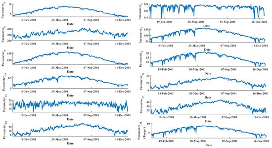
Figure 1.
Parameters evolution for 2001 (for illustration purposes).
Furthermore, to better understand the data available and effectively develop the considered prediction models while considering the seasonality inherent in the data, Table 3 clarifies the average statistical measure of the target irradiance for each month of each year. Looking at Table 3, one can recognize (i) the less variable nature of the target irradiance in each month across all of the years available and (ii) the relatively large irradiance, indeed, in the summer months to the other remaining months. This motivates the individual development of various prediction models for each month of the year to estimate the irradiance of the corresponding months of the following years (one-year ahead).
Table 3.
Statistical characteristics of the target irradiance of each month across the whole available years.
For the estimation task, the overall dataset () (N = 7670 data points/days) was divided into the following three different datasets:
- -
- Training dataset (): this is used for building the investigated prediction algorithms. It comprises 75% of the first = 6574 data points (i.e., of the first 18 years, starting from 2001 till 2018), following the Holdout validation procedure. Thus, consists of = 5752 data points;
- -
- Validation dataset (): this is used for optimizing the built-regression algorithms. It comprises 25% of the first = 6574 data points (i.e., of the first 18 years, starting from 2001 till 2018), following the Holdout validation procedure. Thus, consists of = 1918 data points;
- -
- Test dataset (): this is used for evaluating the built-optimized-regression algorithms. It comprises the latter = 1096 data points (i.e., the remaining 3 years, starting from 2019 till 2021). Thus, consists of = 1096 data points.
2.2. Prediction Methodology
Various linear and nonlinear, intuitive, and complex forecasting algorithms were studied in this work to effectively learn and accurately predict the response parameter (i.e., ALLSKY_SFC_SW_DWN) (Section 2.1). The prediction models were built while considering the available dataset’s inherent monthly seasonality (S-), as clarified in Section 1 (Table 3). Once the prediction models were developed, they were evaluated, and their predictability was compared by resorting to standard, well-known performance metrics (Section 2.3).
To achieve the aforementioned goal, the following prediction models were considered. It is worth mentioning that the former three intuitive prediction models (Section 2.2.1, Section 2.2.3 and Section 2.2.2) and the fourth prediction model (Section 2.2.4) were developed in-house and were optimized using the sole target/response parameters (ALLSKY_SFC_SW_DWN) using MATLAB®. In contrast, the latter prediction models (Section 2.2.5, Section 2.2.6 and Section 2.2.7) were developed and optimized using the Regression Learner toolbox available in MATLAB® [24]. To this end, the principal components (PCs) obtained from the 14 available parameters using the data dimensionality reduction technique and the principal component analysis (PCA) technique (for more details about the PCA, interested readers may refer to [25]) were used to develop the prediction models. The component reduction criterion followed in this work is based on the explained variance of 95% among the whole available inputs/parameters.
2.2.1. Seasonal Naïve (S-N) Prediction Model
This basically assumes that the target irradiance at day of month of year () will be the same (i.e., Naïve) as the irradiance collected on the same chronological day of the same month of the previous year () (i.e., seasonality: lag equals 1), and so on (Equation (1)):
Thus, as the name implies, this approach accounts for the daily, monthly, and yearly seasonality.
2.2.2. Seasonal Simple Average (S-SA) Prediction Model
This basically assumes that the target irradiance at day of month of year () will be the simple average value of the previous irradiances collected on the same chronological day of the same month of the whole previous years () (Equation (2)):
Thus, as the name implies, this approach still accounts for the daily, monthly, and yearly seasonality while considering the historical average values.
2.2.3. Seasonal Simple Moving Average (S-SMA) Prediction Model
It basically assumes that the target irradiance at day of month of year () will be the simple average value of the previous irradiances (i.e., a moving window of size of the -th month) collected on the same chronological day of the same month of the whole previous years (Equation (3)):
The value of each month is optimized by exploring the predictability obtained on the test dataset using various candidates of the value from 1 to 18 (i.e., the whole available training/validation datasets). Still, this approach accounts for the daily, monthly, and yearly seasonality while considering the historical average values computed on a window of size .
2.2.4. Seasonal Nonlinear Auto-Regressive (S-NAR) Prediction Model
Nonlinear Auto-Regressive (NAR) models are frequently used in modeling time series. In fact, this model describes the relationship between the forecasted value to its previous ones until a fixed number of lags [26,27]. Mathematically, it is described as follows:
is a nonlinear complex function, is the number of previous lags and is a modeling error term.
It is worth mentioning that the dataset being used in developing the NAR prediction model has been re-established on a daily basis for 1-day head prediction using the historical corresponding days of the same months (i.e., seasonality). For example, the NAR model has been built to estimate the irradiance at day of month of a year while using the historical time-series data of the previous irradiances collected on the same day of the same month of the previous years.
In this work, the NAR prediction model was optimized using the trial-and-error procedure in terms of the number of hidden neurons. Possible candidates for the number of hidden neurons that span the interval from 1 to 10 were explored. The other settings of the NAR model were kept as per the default settings (e.g., hidden neuron activation function, output activation function, feedback delays, etc.). The best NAR model that achieves the minimum mean squared error (MSE) on a validation dataset (i.e., default split of 15%) will be then selected to predict the irradiance on the test dataset () of the three years (2019–2021).
2.2.5. Seasonal Support Vector Machines (S-SVMs) Prediction Model
Support vector machine (SVM) is categorized under the machine learning (ML) field. The operation principle of SVM is to transform the available information from a nonlinear space into another space with high dimensions with the aim of finding hyper-planes using nonlinear maps [28]. In this work, the SVM prediction model has been optimized using the Bayesian optimization (BO) optimizer, with a default number of iterations (i.e., 30) in terms of:
- -
- Kernel function. Various candidates of the kernel functions were examined, such as Linear, Cubic, etc.;
- -
- Kernel scale. Various candidates of the kernel scale value were examined, such as the values from 0.001 to 1000;
- -
- Box constraint. Various candidates of the box constraint value were examined, such as the values from 0.001 to 1000;
- -
- Epsilon value. Various candidates of the epsilon values were examined, such as the values from 0.001 to 1000.
The best SVM model that achieves the minimum MSE on the validation dataset () will then be selected to predict the irradiance on the test dataset ().
2.2.6. Seasonal Gaussian Process Regression (S-GPR) Prediction Model
Gaussian process regression (GPR) is an almost nonparametric machine learning technique that is found to be powerful in solving prediction problems, such as in the solar energy domain [29]. The basic concept of GPR is built around the calculation of the Pearson correlation coefficient between two variables (explanatory and explained), involving their means and standard deviations (for more details, readers can refer to [29] and the references therein).
In this work, the GPR prediction model was optimized using the Bayesian optimization (BO) optimizer with the default number of iterations (i.e., 30) in terms of:
- -
- Basic function: Various candidates of the kernel functions were examined, such as Zero, Constant, etc.;
- -
- Kernel function: Various candidates of the kernel functions were examined, such as Non-isotropic Exponential, Isotropic Exponential, etc.;
- -
- Kernel scale: Various candidates of the kernel scale values were examined, such as the values from 0.001 to 1000;
- -
- Sigma value: Various candidates of the sigma values were examined, such as the values from 0.001 to 1000.
The best GPR model that achieves the minimum MSE on the validation dataset () will then be selected to predict the irradiance on the test dataset ().
2.2.7. Seasonal Neural Network (S-NN) Prediction Model
Neural networks (NNs) are machine learning techniques inspired by human neurons where information is processed progressively from input to output [30,31,32]. A basic NN is composed of interconnected neurons distributed through different layers. Training a NN involves optimizing the weights and biases in order to minimize the error between the measured observations and those generated by the network. To the best of the authors’ knowledge, the main drawback of a NN is that there is no straightforward procedure to set up the network structure in terms of the number of hidden layers, the number of neurons in each layer, as well as the training parameters (algorithm, epochs, …, etc.).
A trial-and-error procedure was adopted in this study to determine the NN parameters as follows:
- -
- The number of hidden layers: various candidates for the number of hidden layers were examined, such as the values from 1 to 3;
- -
- The number of the corresponding hidden neurons: various candidates for the number of hidden neurons were examined, such as the values from 1 to 300;
- -
- The hidden neuron activation function: various candidates for the activation function were examined, such as Sigmoid, ReLU, etc.;
- -
- Regularization strength: various candidates for regularization strength were examined, such as the values from 1 to 300.
The best NN model that achieves the minimum MSE on the validation dataset () will be then selected to predict the irradiance on the test dataset ().
2.3. Performance Metrics
Various performance metrics are available (in the literature) to evaluate the predictability of the investigated regression models on the test dataset. Among them, the following metrics were considered in this work:
- Root mean square error () [kW-h/m2/day]. It calculates the average difference between the true () and estimated () all-sky surface shortwave downward irradiance on the test dataset (Equation (5)). Thus, values close to 0 are indeed preferable;
- Mean absolute percentage error () [%]. It computes the average absolute percentage difference between the true () and estimated () all-sky surface shortwave downward irradiance on the test dataset (Equation (6)). Thus, values close to 0 are indeed preferable.
3. Results and Discussion
This section presents the application results of the considered prediction models. Firstly, the models were built using the training dataset, optimized using the validation dataset, and evaluated and compared using the test dataset for predicting the all-sky surface shortwave downward irradiance target parameter.
The default/optimal configurations used/identified for the built prediction models vary with the chronological order of the month. For instance, Table 4 reports the default/optimal settings of the built, optimized prediction models at an arbitrary month of a year. For example, the default setting of the S-N is that the lag equals 1 (as per Equation (1)), the default setting of the S-SN is that the window size equals 18 (as per Equation (2)), the optimal setting of the S-SMA is that the window size of the (i.e., January) particular month of 2019 is 13 historical irradiances (from 2018 back to 2006) (as per Equation (3)), and the optimal number of hidden neurons obtained for January of 2019 is two neurons using the time-series data established for the whole of the January months of all the historical years. On the other hand, the prediction models built using the Regression Learner toolbox of Matlab® have also been optimized in terms of data standardization (i.e., the mean = 0 and standard deviation = 1 for each of the extracted PC). Thus, the optimal parameters obtained for January using the S-SVM were linear (kernel function), 0.0050982 (box constraint), and 0.00050602 (Epsilon), with no data standardization; when using the S-GPR, they were linear (basic function), Nonisotropic Matern 5/2 (kernel function), 121.2384 (kernel scale), and 0.0001007 (sigma value), with no data standardization, and using the S-NN, were 2 (number of hidden layers), no hidden neuron activation function, 1.9829 × 10⁻⁷ (regularization strength), and with data standardization.
Table 4.
Default/optimal configurations of the built, optimized prediction models for the validation dataset.
It is worth mentioning that the number of the considered PCs also varies (from 2–4 PCs) for each of the prediction models developed and optimized for each month of the year.
Once the optimal configuration of each prediction model was defined, these were applied to the test “unseen” dataset (i.e., 2019–2021) (Table 5 and Figure 2). For comparison purposes, the reported performance metrics are the average values of the 12 months of each test year.
Table 5.
The average performance metrics obtained by the built, optimized prediction models for the test dataset (i.e., 2019–2021).
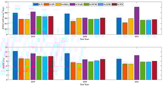
Figure 2.
Bar Chart of the average performance metrics obtained by the built, optimized prediction models for the test dataset (i.e., 2019–2021).
When looking at Table 5 and Figure 2, one can recognize that the performance of the simple, intuitive prediction models, the S-SMA and S-SN, are the best (as indicated in bold in Table 5) in terms of the and the (which takes into account the relative error with respect to the actual/true irradiance value of the target parameter) when compared to the other complex machine learning techniques. Specifically, the performance of the S-SMA seems competitive to the S-SN, as it considers the adaptivity of the window size () that changes/varies for each month of the year, as expected (i.e., of 8.9559% vs. 9.1279% for 2019, 7.0823% vs. 7.4176% for 2020, and 6.7720% vs. 6.8461% for 2021, respectively). In the following rank, the S-GPR achieves good predictability, for instance, when compared to the other nonlinear machine learning algorithms (i.e., S-NN) (i.e., of 9.9317% vs. 10.0809% for 2019, 8.1919% vs. 8.8226% for 2020, and 7.6402% vs. 8.0098% for 2021, respectively). They are followed by the S-SVM and then the S-NAR in terms of the . Last, as expected, the lowest performance was obtained by the traditional S-N prediction model. The justification of the superiority of the best S-SN and S-SMA compared to the S-GPR, for example, is the stable nature of the irradiance across the years that render the development of simple prediction techniques for estimating the irradiance of the upcoming years with negligible computational efforts and costs.
Figure 3 shows the predictions provided by the S-SN, S-SMA, and the S-GPR for the target irradiance of the test dataset, together with its true values; one can clearly notice the effectiveness of the simple, intuitive prediction techniques for predicting the true irradiance accurately compared to the S-GPR.
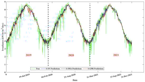
Figure 3.
S-SN, S-SMA, and S-GPR predictions for the test dataset for the irradiance target parameter.
As indicated in the dataset subsection above, the study location (Ha’il province, Saudi Arabia) is a desert region with 80–90% of clear sky days yearly. In order to compare the performance of the best models developed in this study, four references are selected from similar climatic conditions (desert climate) for conducting a comparative study (See Table 6).
Table 6.
Comparison of the results of this study with other studies in similar desert locations.
From the above table, it can be noticed that the results of the present study are comparable to those of other studies conducted in the same climatic conditions. In addition, the models developed in this study are simpler and more efficient since they did not require a lot of calibration or computational effort. Moreover, the algorithmic complexity can be considered to be low.
4. Conclusions
In this study, various naïve and machine learning (ML) approaches were investigated for assessing the potential of photovoltaic solar system yields in a desert climate location in terms of current and future solar irradiance. The obtained results show that the algorithms used were efficient in solving the related forecasting problem based on the daily datasets. In addition, the naïve and simple models slightly outperformed the other methods. Since accurate forecasts are highly desirable for solar energy projects, the results of this study may be used by decision-makers at the national and local energy levels to decide the efficiency of solar energy in replacing classical fossil fuel sources and contribute to environmental sustainability. Although we achieved relatively good results, the proposed approaches may suffer from several limitations, including (i) the difficulty faced when setting the hyperparameters of the algorithms, which is currently performed using time-consuming trial-and-error methods, (ii) the nonavailability of ground-station datasets, and (iii) a low level of generalization since PV yield is highly correlated with clear sky conditions. As such, future works may be devoted to the sizing and implementation of solar energy systems in the Ha’il region, Saudi Arabia, as well as their application in domestic use or for groundwater pumping and desalination.
Author Contributions
Conceptualization, S.B. and S.K.; Methodology, S.A.-D. and S.B.; software, validation, S.A.-D., S.B. and S.K.; formal analysis, W.A.; investigation, L.K.; writing—original draft preparation, S.A.-D. and S.B.; writing—review and editing, L.K., N.B.K., W.A., S.A.-D. and S.K.; visualization, S.A.-D.; supervision, L.K.; funding acquisition, L.K, W.A., S.K. and N.B.K. All authors have read and agreed to the published version of the manuscript.
Funding
This research has been funded by Scientific Research Deanship at University of Ha’il–Saudi Arabia through project number RD-21 024.
Institutional Review Board Statement
Not applicable.
Informed Consent Statement
Not applicable.
Data Availability Statement
The data presented in this study are available on request from the corresponding author. The data are not publicly available due to confidentiality reasons.
Conflicts of Interest
The authors declare no conflict of interest in this work.
Abbreviations
The symbols and acronyms used in this paper are summarized as follows:
| AI | Artificial Intelligence |
| ML | Machine Learning |
| CNN | Convolutional Neural Network |
| SVM | Support Vector Machine |
| GHI | Global Horizontal Irradiation |
| SVC | Support Vector Classifier |
| ANNs | Artificial Neural Networks |
| GA | Genetic Algorithm |
| MLP | Multilayer Perceptron |
| RNNs | Recurrent Neural Networks |
| WO | Wolf Optimization |
| BRNNs | Bayesian Regularized Neural Networks |
| RF | Random Forest |
| SVR | Support Vector Regression |
| PCA | Principal Component Analysis |
| PCs | Principal Components |
| BP | Back-Propagation |
| PSO | Particle Swarm Optimization |
| DE | Differential Evolution |
| DNI | Diffuse Normal Irradiation |
| S-N | Seasonal Naïve |
| S-SA | Seasonal Simple Average |
| S-SMA | Seasonal Simple Moving Average |
| S-NAR | Seasonal Nonlinear Auto-Regressive |
| NAR | Nonlinear Auto-Regressive |
| S-SVMs | Seasonal Support Vector Machines |
| BO | Bayesian Optimization |
| S-GPR | Seasonal Gaussian Process Regression |
| S-NN | Seasonal Neural Network |
| LR | Linear Regression |
| NARX | Nonlinear Auto-Regressive with Exogenous |
| MSE | Mean Squared Error |
| RMSE | Root Mean Square Error |
| MAPE | Mean Absolute Percentage Error |
| R2 | Coefficient of Determination |
| Frequency of data collection | |
| Number of available data points (i.e., days) | |
| Overall matrix | |
| Training dataset | |
| Validation dataset | |
| Test dataset | |
| Number of training data points (i.e., days) | |
| Number of validation data points (i.e., days) | |
| Number of test data points (i.e., days) | |
| Index of the day | |
| Index of the month | |
| Index of the year | |
| Target irradiance at day d of month m of year y | |
| Target irradiance at day d of month m of previous year y − 1 | |
| Number of available years | |
| Moving window size of the m-month | |
| Nonlinear complex function | |
| NAR modeling error term | |
| True irradiance value of the j-th test data point, j = 1, …, Ntest | |
| Estimated irradiance value of the j-th test data point, j = 1, …, Ntest |
References
- Amin, M.; Shah, H.H.; Fareed, A.G.; Khan, W.U.; Chung, E.; Zia, A.; Rahman Farooqi, Z.U.; Lee, C. Hydrogen production through renewable and non-renewable energy processes and their impact on climate change. Int. J. Hydrog. Energy 2022, 47, 33112–33134. [Google Scholar] [CrossRef]
- Lim, S.-C.; Huh, J.-H.; Hong, S.-H.; Park, C.-Y.; Kim, J.-C. Solar Power Forecasting Using CNN-LSTM Hybrid Model. Energies 2022, 15, 8233. [Google Scholar] [CrossRef]
- Theocharides, S.; Makrides, G.; Livera, A.; Theristis, M.; Kaimakis, P.; Georghiou, G.E. Day-ahead photovoltaic power production forecasting methodology based on machine learning and statistical post-processing. Appl. Energy 2020, 268, 115023. [Google Scholar] [CrossRef]
- Gutiérrez, L.; Patiño, J.; Duque-Grisales, E. A Comparison of the Performance of Supervised Learning Algorithms for Solar Power Prediction. Energies 2021, 14, 4424. [Google Scholar] [CrossRef]
- Mohammadi, K.; Shamshirband, S.; Danesh, A.S.; Abdullah, M.S.; Zamani, M. Temperature-based estimation of global solar radiation using soft computing methodologies. Theor. Appl. Climatol. 2016, 125, 101–112. [Google Scholar] [CrossRef]
- Ghazouani, N.; Bawadekji, A.; El-Bary, A.A.; Elewa, M.M.; Becheikh, N.; Alassaf, Y.; Hassan, G.E. Performance Evaluation of Temperature-Based Global Solar Radiation Models—Case Study: Arar City, KSA. Sustainability 2022, 14, 35. [Google Scholar]
- Alghamdi, H.A. A Time Series Forecasting of Global Horizontal Irradiance on Geographical Data of Najran Saudi Arabia. Energies 2022, 15, 928. [Google Scholar] [CrossRef]
- Hafdaoui, H.; Boudjelthia, E.A.K.; Chahtou, A.; Bouchakour, S.; Belhaouas, N. Analyzing the performance of photovoltaic systems using support vector machine classifier. Sustain. Energy Grids Netw. 2022, 29, 100592. [Google Scholar] [CrossRef]
- Mohana, M.; Saidi, A.S.; Alelyani, S.; Alshayeb, M.J.; Basha, S.; Anqi, A.E. Small-Scale Solar Photovoltaic Power Prediction for Residential Load in Saudi Arabia Using Machine Learning. Energies 2021, 14, 6759. [Google Scholar] [CrossRef]
- Khalyasmaa, A.I.; Eroshenko, S.A.; Tashchilin, V.A.; Ramachandran, H.; Piepur Chakravarthi, T.; Butusov, D.N. Industry Experience of Developing Day-Ahead Photovoltaic Plant Forecasting System Based on Machine Learning. Remote Sens. 2020, 12, 3420. [Google Scholar] [CrossRef]
- Rodríguez, F.; Martín, F.; Fontán, L.; Galarza, A. Ensemble of machine learning and spatiotemporal parameters to forecast very short-term solar irradiation to compute photovoltaic generators’ output power. Energy 2021, 229, 120647. [Google Scholar] [CrossRef]
- Jia, D.; Yang, L.; Lv, T.; Liu, W.; Gao, X.; Zhou, J. Evaluation of machine learning models for predicting daily global and diffuse solar radiation under different weather/pollution conditions. Renew. Energy 2022, 187, 896–906. [Google Scholar] [CrossRef]
- Rana, M.; Rahman, A. Multiple steps ahead solar photovoltaic power forecasting based on univariate machine learning models and data re-sampling. Sustain. Energy Grids Netw. 2020, 21, 100286. [Google Scholar] [CrossRef]
- Feng, Y.; Gong, D.; Zhang, Q.; Jiang, S.; Zhao, L.; Cui, N. Evaluation of temperature-based machine learning and empirical models for predicting daily global solar radiation. Energy Convers. Manag. 2019, 198, 111780. [Google Scholar] [CrossRef]
- Nourani, V.; Elkiran, G.; Abdullahi, J.; Tahsin, A. Multi-region Modeling of Daily Global Solar Radiation with Artificial Intelligence Ensemble. Nat. Resour. Res. 2019, 28, 1217–1238. [Google Scholar] [CrossRef]
- Jahani, B.; Mohammadi, B. A comparison between the application of empirical and ANN methods for estimation of daily global solar radiation in Iran. Theor. Appl. Climatol. 2019, 137, 1257–1269. [Google Scholar] [CrossRef]
- Vaisakh, T.; Jayabarathi, R. Analysis on intelligent machine learning enabled with meta-heuristic algorithms for solar irradiance prediction. Evol. Intell. 2022, 15, 235–254. [Google Scholar] [CrossRef]
- Chahboun, S.; Maaroufi, M. Principal Component Analysis and Machine Learning Approaches for Photovoltaic Power Prediction: A Comparative Study. Appl. Sci. 2021, 11, 7943. [Google Scholar] [CrossRef]
- Zhang, Y.; Cui, N.; Feng, Y.; Gong, D.; Hu, X. Comparison of BP, PSO-BP and statistical models for predicting daily global solar radiation in arid Northwest China. Comput. Electron. Agric. 2019, 164, 104905. [Google Scholar] [CrossRef]
- Babatunde, O.M.; Munda, J.L.; Hamam, Y. Exploring the Potentials of Artificial Neural Network Trained with Differential Evolution for Estimating Global Solar Radiation. Energies 2020, 13, 2488. [Google Scholar] [CrossRef]
- Ramos, L.; Colnago, M.; Casaca, W. Data-driven analysis and machine learning for energy prediction in distributed photovoltaic generation plants: A case study in Queensland, Australia. Energy Rep. 2022, 8, 745–751. [Google Scholar] [CrossRef]
- Maitanova, N.; Telle, J.-S.; Hanke, B.; Grottke, M.; Schmidt, T.; Maydell, K.V.; Agert, C. A Machine Learning Approach to Low-Cost Photovoltaic Power Prediction Based on Publicly Available Weather Reports. Energies 2020, 13, 735. [Google Scholar] [CrossRef]
- Pasion, C.; Wagner, T.; Koschnick, C.; Schuldt, S.; Williams, J.; Hallinan, K. Machine Learning Modeling of Horizontal Photovoltaics Using Weather and Location Data. Energies 2020, 13, 2570. [Google Scholar] [CrossRef]
- MATLAB Regression Learner App. Available online: https://www.mathworks.com/help/stats/regression-learner-app.html (accessed on 10 October 2022).
- Jolliffe, I.T. Principal Component Analysis. J. Am. Stat. Assoc. 2002, 98, 487. [Google Scholar]
- Louzazni, M.; Mosalam, H.; Khouya, A. A non-linear auto-regressive exogenous method to forecast the photovoltaic power output. Sustain. Energy Technol. Assess. 2020, 38, 100670. [Google Scholar] [CrossRef]
- Fentis, A.; Bahatti, L.; Tabaa, M.; Mestari, M. Short-term nonlinear autoregressive photovoltaic power forecasting using statistical learning approaches and in-situ observations. Int. J. Energy Environ. Eng. 2019, 10, 189–206. [Google Scholar] [CrossRef]
- Zendehboudi, A.; Baseer, M.A.; Saidur, R. Application of support vector machine models for forecasting solar and wind energy resources: A review. J. Clean. Prod. 2018, 199, 272–285. [Google Scholar] [CrossRef]
- Najibi, F.; Apostolopoulou, D.; Alonso, E. Enhanced performance Gaussian process regression for probabilistic short-term solar output forecast. Int. J. Electr. Power Energy Syst. 2021, 130, 106916. [Google Scholar] [CrossRef]
- Al-Dahidi, S.; Ayadi, O.; Adeeb, J.; Louzazni, M. Assessment of Artificial Neural Networks Learning Algorithms and Training Datasets for Solar Photovoltaic Power Production Prediction. Front. Energy Res. 2019, 7, 130. [Google Scholar] [CrossRef]
- Al-Dahidi, S.; Ayadi, O.; Alrbai, M.; Adeeb, J. Ensemble approach of optimized artificial neural networks for solar photovoltaic power prediction. IEEE Access 2019, 7, 81741–81758. [Google Scholar] [CrossRef]
- Al-Dahidi, S.; Louzazni, M.; Omran, N. A Local Training Strategy-based Artificial Neural Network for Predicting the Power Production of Solar Photovoltaic Systems. IEEE Access 2020, 8, 150262–150281. [Google Scholar] [CrossRef]
- Jebli, I.; Belouadha, F.-Z.; Kabbaji, M.I.; Tilioua, A. Prediction of solar energy guided by pearson correlation using machine learning. Energy 2021, 224, 120109. [Google Scholar] [CrossRef]
- Hassan, M.A.; Bailek, N.; Bouchouicha, K.; Nwokolo, S.C. Ultra-short-term exogenous forecasting of photovoltaic power production using genetically optimized non-linear auto-regressive recurrent neural networks. Renew. Energy 2021, 171, 191–209. [Google Scholar] [CrossRef]
- McCandless, T.; Dettling, S.; Haupt, S.E. Comparison of Implicit vs. Explicit Regime Identification in Machine Learning Methods for Solar Irradiance Prediction. Energies 2020, 13, 689. [Google Scholar] [CrossRef]
- Blal, M.; Khelifi, S.; Dabou, R.; Sahouane, N.; Slimani, A.; Rouabhia, A.; Ziane, A.; Neçaibia, A.; Bouraiou, A.; Tidjar, B. A prediction models for estimating global solar radiation and evaluation meteorological effect on solar radiation potential under several weather conditions at the surface of Adrar environment. Measurement 2020, 152, 107348. [Google Scholar] [CrossRef]
Disclaimer/Publisher’s Note: The statements, opinions and data contained in all publications are solely those of the individual author(s) and contributor(s) and not of MDPI and/or the editor(s). MDPI and/or the editor(s) disclaim responsibility for any injury to people or property resulting from any ideas, methods, instructions or products referred to in the content. |
© 2022 by the authors. Licensee MDPI, Basel, Switzerland. This article is an open access article distributed under the terms and conditions of the Creative Commons Attribution (CC BY) license (https://creativecommons.org/licenses/by/4.0/).