Article

Passenger Travel Path Selection Based on the Characteristic Value of Transport Services

1
School of Economics and Management, Civil Aviation Flight University of China, Guanghan 618307, China
2
School of Airport, Civil Aviation Flight University of China, Guanghan 618307, China
3
Scientific Research Department, Civil Aviation Flight University of China, Guanghan 618307, China
4
Scientific Base of Flying Technology and Safety, Civil Aviation Flight University of China, Guanghan 618307, China
*
Author to whom correspondence should be addressed.
Sustainability 2023, 15(1), 636; https://doi.org/10.3390/su15010636
Submission received: 19 November 2022 / Revised: 24 December 2022 / Accepted: 27 December 2022 / Published: 30 December 2022
(This article belongs to the Collection Sustainable Transport Economics, Behaviour and Policy)

Abstract

:
In this paper, we establish a generalized cost function for passenger travel based on the characteristic value of transportation services, and we select high-speed rail, air, and air–rail as the selection branches in order to build a passenger travel decision-making model combined with a logit model to analyze the preference for passenger travel choices. The results show that, within the transportation network of the Chengdu–Chongqing economic circle, passengers are more likely to take the high-speed rail option directly, followed by air–rail and air options, and these results are concentrated within a transportation distance range of less than 1000 km, 1000–1200 km, and more than 1200 km, respectively. Among them, the OD travel routes comprised Chengdu and Yibin as the transit nodes of the combined travel account for more than 50%, which exhibits the high strategic development potential of air–rail combined transportation. Ridge regression analyses show that ticket price, quickness, convenience, and comfort influence the probability related to travelers’ travel choice at varying degrees. The elasticity values of the fatigue recovery time, travel time, and time value per capita for high-speed rail are much greater than the other two travel modes, indicating that these three factors have a high impact on the travel choice behavior of high-speed rail.

1. Introduction

With the continuous improvement of the national economy and transportation system, the purpose of passengers’ travel is not only to work and return home. When basic travel needs are met, people are increasingly seeking social and spiritual satisfaction, resulting in a “qualitative” increase in travel demands such as vacation, visiting relatives, and friends [1]. Therefore, a single mode of transportation no longer satisfies the personalized travel of passengers. In the travel situation where passengers have multiple choices, there are fierce competitions among different transportation modes for the source of passengers. Within the range of 650–750 km, high-speed rail transport has a significant impact on the air passenger transport market, and with the increase in flight distance, the impact of high-speed rail on aviation gradually decreases [2]. However, in terms of transport structure, there are complementarities between the two. A large number of scholars started to study the air–rail intermodal component of the integrated transportation system [3,4]. Thus, it is important to study passenger travel choice behavior in terms of measuring the market advantages of different transportation modes and the rationality of resource allocation.
Currently, research on passenger travel behavior is mainly carried out from the following perspectives: the influence of price, time, and other attributes of transportation modes on selection behavior. Sun et al. studied competitive and cooperative effects between air transport and high-speed rail in different regions within ten countries and observed that the travel time is a key factor influencing travelers’ travel choices, and it is also an important driver of the success of high-speed rail and air travel [5]. In addition, Pagliara et al. [6] studied the travel behavior of Madrid and Barcelona passengers by establishing a competitive mode for travel choice models, and they observed that price is an important factor in passenger choice. The least-expected travel-time path on random and time-dependent networks is a problem that requires finding the path between the origin and destination to ensure the minimum expected travel time within a given departure time. Based on this, Yamín et al. [7] proposed an extension of the pulse algorithm to explore the path. From the perspective of complex systems, Hu et al. [8] divided the overall time series into time intervals and expressed the path cost as a time variable, and they applied the utility function to propose an efficient and robust solution for passenger travel path selection. Feng et al. [9] constructed a generalized cost function that considers factors such as travel time, fare, transfer penalties, comfort, and safety, providing academic support for future travel mode selections and improved travel planning. Wang et al. [10] used structural equations to explore the influence of potential factors on travelers’ travel mode choice, and the results showed that travel distances have a significant influence on path and travel mode choices. The influence of socio-economic levels and geographical conditions on selection behavior was examined. The research results showed that the higher the level of regional economic development, the more developed its air transport will be [2]. Moreover, the development of high-speed rails has a positive impact on air transport, and its substitution effect cannot be underestimated. Wang et al. [11] analyzed the impact of high-speed rail on civil aviation in the hinterland of the overlapping services of high-speed rail and civil aviation based on GIS, and they provided relevant suggestions for future construction. At the same time, relevant scholars further expanded their research to dynamically capture the travel behavior of passengers and make the corresponding market adjustments. In the consideration of the competition between airlines and high-speed railways under different modes, Cadarso et al. [12] used the integrated mixed integer nonlinear optimization model to generate airline schedules to analyze the impact of decision making on passenger demands, and they used a nested logit model to estimate the demand related to a given plan in order to change the flight schedules, fleet composition changes, and ticket price changes to effectively cope with the progression of high-speed railways. Su et al. used binary logit to explore the mode choice patterns in the Beijing–Shanghai corridor. The results reveal the travel characteristics of passengers between Beijing and Shanghai and provided information for policy design and infrastructure management [13]. Scholars analyzed the use of the high-speed rail in Taiwan and China in the past 8 years, and they developed ten graphical long-term use patterns with detailed use descriptions to capture the behavioral dynamics of some samples and to explain them to some extent [14]. The above research studies mainly focused on time, cost, and external environmental factors to study the travel behavior of passengers or the choice behavior of passengers for a certain transportation mode. Therefore, the current research on passenger travel behavior has the following gaps: the coordination between individual passengers and transport service attributes has not been taken into account, and the air–rail complementarity has not been taken into account to generate an air–rail intermodal transport choice.
In view of this, this paper provides the following innovations to address the gaps in the above research areas: (1) We combine the individual time value of passengers with transport service attributes, quantify it as the characteristic value that passengers need to pay for travel, and establish a generalized cost function. (2) The path under the scenario of using the air–rail combination (air and high-speed rail) as the travel tool is selected as the passenger travel decision-making limb. We analyze the preference of passengers for different travel paths in the context of having multiple choices in order to describe the travel behavior of passengers. Therefore, based on the perspective of passenger travel, we analyze passengers’ preference for travel paths comprising different transport modes, which, on the one hand, makes up for the current research situation that mainly focuses on the travel choice behavior given the air–rail competition while ignoring the complementarity between high-speed rail and aviation. On the other hand, we combine the generalized time cost generated by transport modes with the individual time value of passengers, and we convert it into specific monetary performance; this is the main consideration for passenger decision making. This action reasonably evaluated the preferences of passengers in the transport market for travel paths; effectively described whether the delivery of transport resources matched the utilization of market resources, reflecting the strategic position of transport modes in the passenger transport market; and provided strong guidance for the subsequent network construction and resource allocation of transport enterprises.
The paper is structured as follows: Section 1 is an introduction, which introduces the background and significance of the study and reviews the current status and shortcomings of the study. Section 2 presents the research methodology. Section 3 includes the passenger travel path, passenger travel preference analysis, ridge regression analysis, and the sensitivity analysis of influencing factors. Section 4 includes the conclusion and the study’s implications.

2. Methods

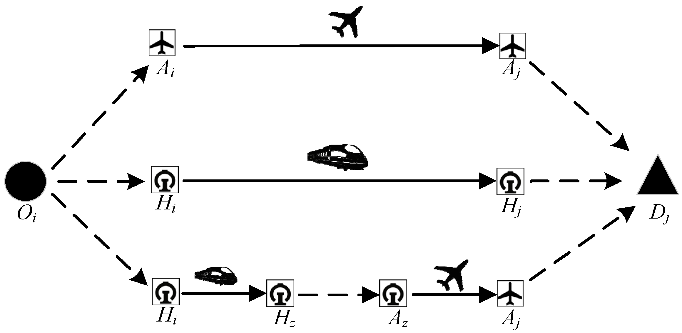
2.1. Path Scenario Setting

G = (N, M) represents the network of passenger travel, and N is the node set, including the high-speed railway stations, airports, and other transport hubs. M is the origin-destination (OD) travel route, representing the connecting line formed between the transportation nodes. On an OD travel route, L(OD) is the set of all possible paths from the starting point Oi to the ending point Dj, and Lmin is recorded as the path with the least amount of travel expenses paid by passengers. The connecting travel mode at both ends of OD is urban traffic. Then, the travel path between Oi and Dj exhibits the following situations, as shown in Figure 1.
(1) Air direct (A): Here, passengers directly choose air transport to travel between station Ai and station Aj.
(2) High-speed rail direct (H): Here, passengers directly choose high-speed rail to travel between station Hi and station Hj.
(3) Air–rail combination (HA): Passengers choose the high-speed rail to travel from station Hi to station Hz, transfer to station Az by means of urban transportation, and travel to station Aj by air. The travel sequence of the air–rail combination can be ordered as air travel first and then high-speed rail travel.

2.2. Generalized Cost Function

As economies develop dramatically faster, passengers often choose the travel path that can maximize their interests according to their own economic conditions, the attributes of transportation, and travel purposes when they have multiple paths to choose from. The generalized cost generated during the entire travel process refers to the total cost paid by passengers in the travel stage, including the ticket price and the characteristic cost generated by other attributes of the transport mode. That is, when passengers generate demands, the benefit increment obtained during travel times and the non-productive time consumed when traveling comprise monetary performance [15]. Given this, this paper introduces the concept of per capita time value. The per capita time value (A) is measured by the income method used in economics, which is the ratio of per capita GDP to the annual working time. For passengers, their travel comprises the process of maximizing their interests. Therefore, whether the unit time value and economic affordability of individual passengers can adapt to the time and monetary consumption generated in the actual travel process has become an important factor for passengers to consider.
With gradual improvements in high-speed rail and civil aviation transport networks, the strategic focus of the current transport system shifted from developing quantity to quality. To some extent, the characteristic costs incurred due to the attributes of transport modes have an important impact on the psychological satisfaction of passengers and their willingness to ride that particular transport mode again. From the perspective of passenger travel, the reasonable quantification of additional costs incurred by different transport attributes for passengers can effectively analyze the preferences of passengers for different travel modes, reflecting the transport status of different travel paths in the current passenger transport market. However, many factors affect passenger travel. According to existing research results, this chapter summarizes the attributes of transportation modes other than ticket price within the areas of quickness, convenience, comfort, and security.

2.2.1. Ticket Price (E)

Currently, the railway transport enterprises mainly formulate published fares according to the notice on reforming and improving the passenger fare policy of high-speed railway. The assignment methods of air fares are mainly divided into two categories: according to the notice on further improving the domestic air transport price policy of civil aviation. The measurement rules of domestic airline passenger transport fares that continue to implement the government’s suggested price in the document are shown in Equation (1). For domestic passenger transport fares with market-adjusted prices, the fares published on the official website are directly used as statistical indicators.
{ I c o m = L O G ( 150 , D I S i × 0.6 ) × D I S i × 1.1 I p l a = L O G ( 150 , D I S i × 0.6 ) × D I S i × 1.3
Icom and Ipla are the fares of ordinary routes and plateau routes, respectively, and DISi is the route’s distance.

2.2.2. Quickness (Q)

Speed is mainly measured by travel times, which mainly comprise two parts: the travel time of taking the main means of travel such as plane or high-speed rail (main time spent in travel) and the sum of the travel time and transfer time with respect to urban traffic at both ends of OD (travel time of connecting vehicles). In terms of the main time spent when traveling, due to the topography and scale of the transport network, the actual travel distance and time consumed with respect to high-speed rail passengers are somewhat different from those expected. Therefore, compared with air transport with super plane transport characteristics, high-speed rail transport takes longer on the same OD route. As for the travel time consumption of the connection mode, the layout of high-speed rail stations is mainly concentrated within urban areas. The connection between urban traffic and high-speed rail stations in most cities has been relatively perfect, providing high accessibility for passengers. However, air transport is affected by special factors such as safety management levels. Airports are mainly distributed in the suburbs, which are located at a certain distance from the city and have relatively poor connections with urban traffic. Therefore, the travel time of the air transport connection mode is longer than that of the high-speed rail.
Q k = ( T k + t ) × V
Tk is the travel time of the transportation mode K, t is the sum of the travel time and transfer time in the cities at both ends, and V is the per capita time value.

2.2.3. Convenience (F)

In the early stage of travel preparation, passengers consider the complexity of ticket purchase, transit, security check, waiting, and other processes, which determine the travel time reserved for passengers. Therefore, the time cost value generated at this stage is also an important part of the cost expenditure. It has a great impact on the travel journey of passengers with respect to high time sensitivity [16]. Intercity transportation with high-speed rail as the travel mode gradually tended to comprise “public transportation”; i.e., the interval between the departure stations is shortened. Although some stations are limited by the level of urbanization, the departure interval is still long, but time consumption is relatively short compared to the more complicated boarding processes air transportation.
F k = T y k × V
Tyk is the travel reservation time required for taking the transportation mode K.

2.2.4. Comfort (C)

Passengers are predisposed to fatigue to a certain extent when they travel, so the time spent by passengers to recover from fatigue represents the comfort level of the travel mode.
{ t k = 15 1 + a × e b × T k C k = t k × V
tk is the fatigue recovery time, and a and b are the retardation coefficients, respectively.

2.2.5. Security (S)

As the most basic and important criterion of transportation products, safety is the first travel factor that passengers consider in addition to other factors. With the implementation of security measures, the popularization of education, and the inspection of the authorities, the passenger travel safety factor is maintained at a high level. Therefore, the safety index is 1.
To summarize, if the expenditure cost of the k-th path selected on the OD travel route is Uk, then the generalized cost function of passenger travel can be expressed, as shown in Equation (5).
U k = ( θ 1 E + θ 2 Q + θ 3 F + θ 4 C ) × S
θi is the characteristic parameter corresponding to the service attribute of the transport mode, which measures the importance of different transport service characteristics in the process of passenger travel selection to some extent, and it is solved by the maximum likelihood estimation method.

2.3. Travel Path Selection Probability Model

When there are multiple selection limbs, the probability that the k-th travel path on the OD route is selected and is denoted as Pk. Since exponential growth can easily cause substantial difference in the results, the generalized cost is averaged. The maximum probability path may represent the optimal travel choice of the passenger.
{ p k = exp ( U k / U ¯ ) 1 k exp ( U k / U ¯ ) U ¯ = 1 k U k / k

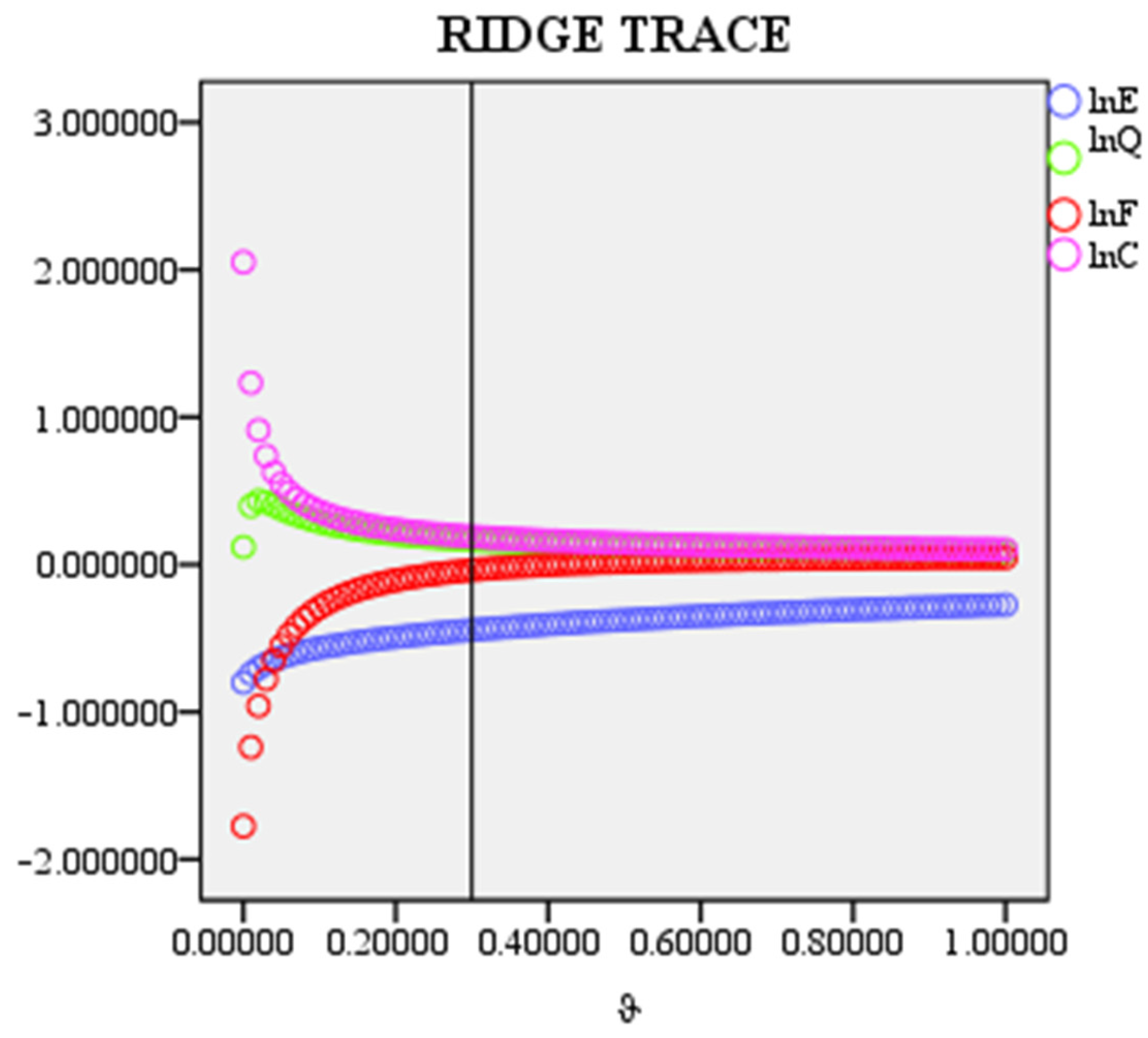
2.4. Ridge Regression Model

When there is a strong correlation between the explanatory variables, fitting using general regression methods can result in large errors. When passenger travel choices are analyzed, indicators such as ticket price (E), quickness (Q), convenience (F), and comfort (C) are often selected from the perspectives of the transport economy, travel fares, and travel distance. Most of these indicators have multicollinearity among them, which seriously affects the accuracy of the estimation’s results [17]. However, ridge regression has a unique advantage in dealing with multicollinearity problems [18].
Analyzing the linear regression equation from the point of view of the general form by = Y, we can obtain β = ( X X ) 1 X Y , where X′ is the transpose matrix of X. Due to the presence of multicollinearity, the X matrix is not of full rank (i.e., | X X | = 0 ). Therefore, error reductions are achieved by constructing the X X + ϑ I matrix, where I is the unit matrix. After completion, the ridge regression model is shown below:
β = ( X X + ϑ I ) 1 X Y ,
where ϑ is the ridge regression parameter, and ϑ > 0 .

3. Case Analysis

3.1. Travel Route Screening

In the “National Comprehensive Three-dimensional Transport Network Planning Outline”, it was proposed that the Chengdu–Chongqing economic circle, Beijing–Tianjin-Hebei economic circle, Yangtze River Delta city group, and Guangdong–Hong Kong–Macao bay area should be listed as “four poles” to build four comprehensive transport hub clusters. With the continuous improvement of the regional transportation network, the passenger’s choice of travel path gradually diversified. In order to attract customers, different transportation enterprises launched corresponding market competitions, which introduced changes in the structure of the transportation market to a certain extent.
In view of this, in this paper, we take Chengdu and Chongqing as the core areas; Yibin, Dazhou, Mianyang, Deyang, Leshan, Luzhou, and Nanchong as the regional centers; and the Chengdu–Chongqing economic circle as the study’s object. Prefecture-level cities comprise the basic research unit. Among them, the statistical scale of the high-speed railway data comprises G/D/C trains, which are derived from the train’s timetable. Aviation data are derived from the national flight schedule published by the civil aviation administration of China. The social data are mainly derived from the 2021 national statistical yearbook of China.
In order to study the selection probability of different paths for passengers in the context of diversified travel choices, the travel traffic network includes cities with high-speed rail stations and airports as nodes, and the OD routes with high-speed rail, air, and air–rail combined travel are taken as edges. If there are multiple high-speed railway stations or airports in the city, the data will be merged. For example, the Nanjing railway station and Nanjing south railway station will be merged into Nanjing; the Shanghai Hongqiao airport and Shanghai Pudong airport will be merged into Shanghai. Finally, 67 OD routes and 316 travel paths were obtained in 2021.
As shown in Figure 2, the spatial layout of the outbound travel routes of the passengers in the Chengdu–Chongqing economic circle is fan-shaped. With the urban nodes in the system as the starting points, the spatial distribution of the OD travel routes with three travel paths is mainly concentrated in the central region and coastal areas, which indicates that the construction of its comprehensive transportation system with the western region and the northeast region is not perfect. At the same time, as far as OD travel routes are concerned, the number of travel paths that passengers can choose from with respect to different routes varies to a certain extent. There are many 6–7 route choices for destinations in first tier cities such as Beijing, Guangzhou, and Shanghai, while there are only a few path choices for destinations in urban nodes located in marginal areas.

3.2. Analysis of Passenger Travel Preference

Based on the characteristic value generated by the attribute of the transportation mode, a passenger travel decision-making model of the Chengdu–Chongqing economic circle is constructed to analyze the travel preference of passengers on different travel paths.
As shown in Figure 3, the OD connection’s starting nodes with three travel scenarios are mainly distributed in Chongqing, Chengdu, Yibin, and Mianyang. Among them, the OD connections for which passengers can complete air–rail combined travel from Chengdu and Yibin account for 26.9% and 23.3% of the total, respectively, which confers high strategic development potential for this type of node for air–rail combined transport. In the entire travel transportation network, the probability of passengers choosing the first mode from high to low is high-speed rail, air–rail combined travel, and air. High-speed rail transportation occupies a large advantage in the regional market. From the perspective of distance distribution, direct travel by using high-speed rail, air direct, and air–rail combinations is mainly concentrated within a transport range of less than 1000 km, 1000–1200 km, and more than 1200 km, respectively, indicating that from the perspective of passenger travel, high-speed rail provides more service advantage in the medium- and short-range transport market, while air transport and air–rail combined transport occupy an important market position in the medium- and long-range transport market. At the same time, it explains the travel preference of passengers for different transportation modes in terms of transportation distances.
From the perspective of different transport modes, among the path samples of the overall OD travel routes, there are 67 travel paths comprising direct high-speed rail as the transport mode, and 32 are finally selected as the optimal travel paths by passengers. There are 67 travel paths with direct air transportation as the transport mode, and 13 are finally selected as the optimal travel paths by passengers. There are 316 travel paths in total with the air–rail combination as the transport mode, and 22 are finally selected as the optimal travel paths by passengers. The number of various travel paths is regarded as the market launch of transport products, and the final choice of passengers is regarded as the product usage of various travel paths. It was found that the market utilization rate of high-speed rail direct transportation is as high as 47.8%, the market utilization rate of air direct transportation is moderate, at 19.4%, and the utilization rate of air–rail combination travel paths is only 7%. However, according to the fact that there is only one optimal travel path for each OD route, among the 67 optimal travel paths, 47.8% of passengers finally decided to take high-speed rail for direct travel, 19.4% for air direct travel, and 32.8% for air–rail combination travel. It can be seen from this that in the passenger transport market with passengers as the main body, although the utilization rate of air–rail combination travel resources is low, it still plays an indispensable role in the overall passenger transport market.
To sum up, according to the characteristic costs generated by the vehicle’s attributes, passengers should combine their own unit time values to decide on travel behaviors that can maximize their interests. In the Chengdu–Chongqing economic circle, high-speed rail is directly connected to meet nearly half of the travel demands of the passenger transport market. At the same time, it is found that air–rail combination travel plays an important role in the daily travel of residents. This new travel mode, to a certain extent, integrates the transport advantages of high-speed rail and air, making it more popular with passengers within the medium and long travel distance range.

3.3. Regression Analysis

This section attempts to investigate the extent to which ticket price (E), quickness (Q), convenience (F), and comfort (C) affect the probability related to passenger travel choices under different travel modes (air direct, high-speed rail direct, air–rail combination direct) by using a ridge regression model, thus providing a theoretical as well as empirical basis for the design of different types of passenger service products by air and high-speed rail.

3.3.1. Multicollinearity Test

The variance inflation factor (VIF) is used to test for the presence of multicollinearity between variables in general, and it is an indicator of covariance between variables, essentially measuring the correlation between variables. The variance inflation factor is shown in Equation (8).
V I F i = 1 1 R i 2
R i 2 represents the square of the complex correlation coefficient obtained by regressing the independent variable Xi on all other independent variables. The criterion for judging multicollinearity, VIF > 5, is a very strict requirement; VIF > 10 is a more relaxed requirement. In this paper, VIF > 5 was chosen as the criterion for judging multicollinearity [18].
The results of the multicollinearity test are shown in Table 1. We used stata17.0 software to calculate VIF to test for multicollinearity. The results show that the VIF values of lnQ, lnF, and lnC are all greater than 5 under the three travel modes comprising air direct, high-speed rail direct, and air–rail combination direct, which indicates the existence of multicollinearity among the independent variables. Therefore, according to the basic theory of econometrics, the general econometric regression model is not applicable to the analysis of the impact factors in this study. We therefore considered using a ridge regression model.

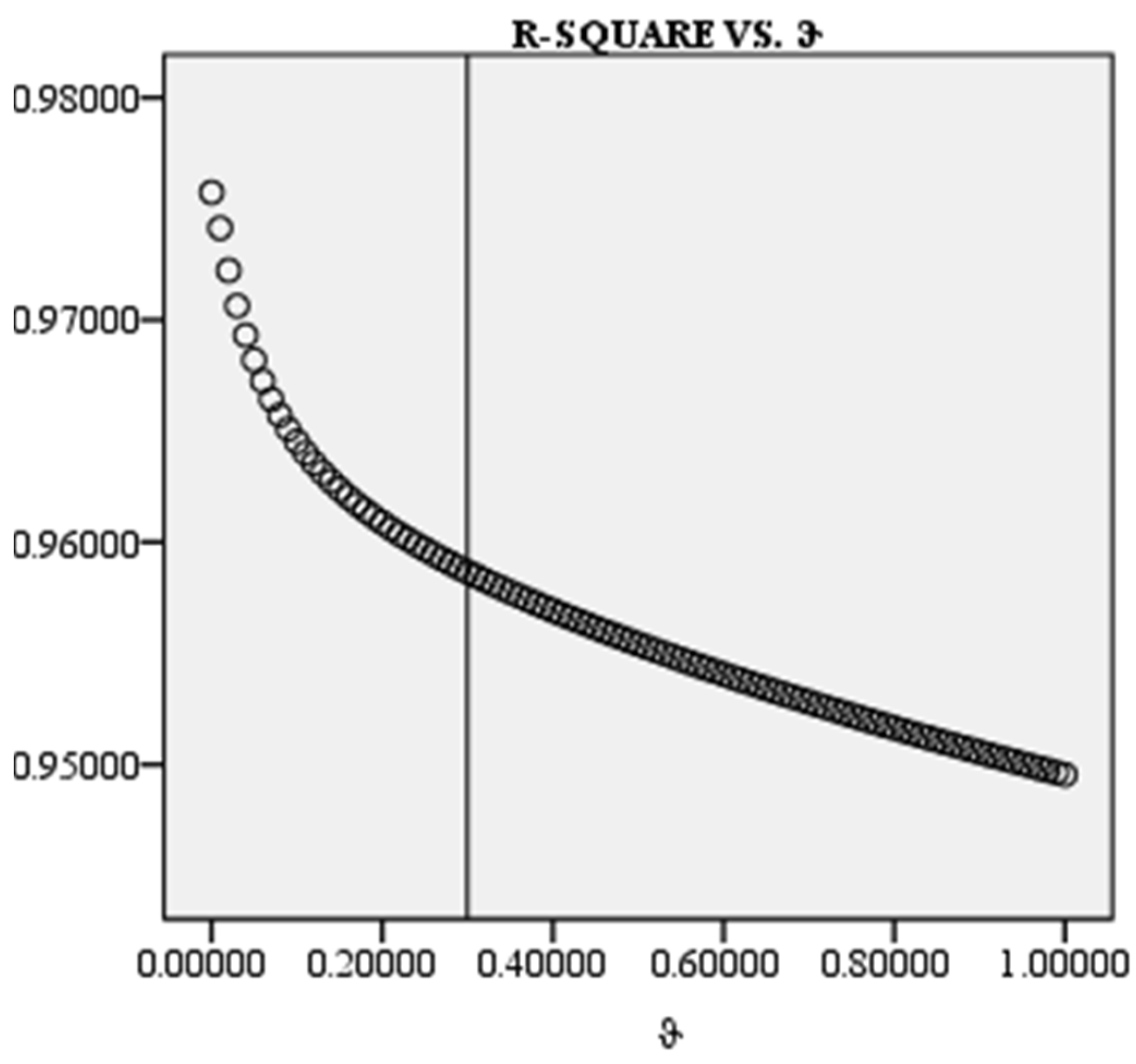
3.3.2. Ridge Regression Estimation

Since there is serious multicollinearity among the variables lnE, lnQ, lnF and lnC, and the variables have a non-negligible effect on the choice of travel routes of passengers, a ridge regression analysis was used to explain the influence of different variables on the travel choices of passengers. To a certain extent, it can eliminate the problems of unsatisfactory and insignificant regression results caused by multicollinearity. In order to reduce the effect of heteroskedasticity on the model and errors in data processing, we take logarithms for the independent variables in the model. The model is constructed as follows:
ln P h = β 0 + β 1 ln E h + β 2 ln Q h + β 3 ln F h + β 4 ln C h + ε ,
where Ph denotes the probability of choosing travel mode h; Eh, Qh, Fh, and Ch denote the attributes of ticket price, quickness, convenience, and comfort on travel mode h, respectively (h = A, H, HA); β0, β1, β2, β3, and β4 are coefficient estimates; ε is the random error term.
The study was first conducted to address the impact of air travel choices. In this study, a ridge regression analysis was carried out by writing a program using SPSS 20.0. Setting the ridge regression coefficient ϑ between (0, 1) and a step size of 0.01, a ridge plot is obtained (Figure 4) along with a trend plot of the change in the decidability coefficient, R2, with the value of ϑ (Figure 5). It can be observed from Figure 4 that the ridge-trace plot changes gradually and smoothly when ϑ ≥ 0.3 and that the regression coefficients and R2 of the respective variables tend to stabilize. Therefore, in this paper, k = 0.3 is taken as the fitting result of the ridge regression, and this is used to determine the ridge regression equation.
As can be seen in Figure 5, R2 is always greater than 0.95 when the value of ϑ is between 0 and 1. This indicates that the explanatory strength of the respective variable for the dependent variable is greater than 0.95 whenever ϑ takes values between 0 and 1, which has a good explanatory power. The details are shown in Table 2.
In addition, high-speed rail direct transport is judged in the same manner as HA direct; thus, it will not be repeated here. The final ridge regression results for A, HA, and H are summarized in Table 3.
As can be seen in Table 3, almost all parameters are significant for all three modes of travel. The corresponding ridge regression equation is presented as follows.
ln P A = 0.37 + 0.224 ln E A + 0.235 ln Q A + 0.239 ln F A + 0.243 ln C A ,
ln P H = 0.747 + 0.23 ln E H + 0.233 ln Q H + 0.242 ln F H + 0.24 ln C H ,
ln P H A = 0.312 ln E H A + 0.061 ln Q H A 0.036 ln F H A + 0.095 ln C H A .

3.3.3. Results Analysis of Ridge Regression

As shown in Table 3 and Equations (10)–(12), the results of the ridge regression show the following: (1) Comfort (lnC) has the greatest impact on the probability of passengers in choosing air direct, and it is slightly higher than the impact on the probability of choosing high-speed rail direct. Specifically, a 1% increase in lnC increases the probability of choosing air direct access by 0.243% and the probability of choosing high-speed rail direct access by 0.240%. The reason for this phenomenon is mainly due to the fact that as people’s living standards improve, the focus of travel concerns gradually shifts to the comfort of the travel transportation mode, and comfort with respect to air transportation is particularly important. This finding echoes the study of İmre et al. [19]. (2) Convenience (lnF) had the largest effect on the probability of choosing direct access by high-Speed rail, which is slightly higher than the effect on the probability of choosing direct access by air, but it was not significant for the probability of choosing HA. Specifically, a 1% increase in lnF increases the probability of travelers choosing direct high-speed rail travel by 0.242%, while the probability of choosing direct air travel increases by 0.239%. The main reason for this phenomenon is that airports are often located far away from urban areas, requiring early departure for air travel, long pre-trip preparation times, and easy delays. Thus, the convenience of air direct travel is to some extent lower than that of HSR direct. the convenience of HA is the lowest, so the effect of lnF on HA is not significant. (3) Quickness (lnQ) has the greatest effect on the probability of a traveler choosing air direct, while it hardly affects the probability of choosing HA travel. Specifically, when lnQ increased by 1%, the probability of choosing air direct increased by 0.235%, while the probability of choosing HA travel increased by 0.061%. (4) The effect of ticket price (lnE) on the probability of the travel choice of passengers is observed when ticket prices increase. Passengers are least inclined to choose HA travel. In contrast, the effect on the choice of air direct travel is relatively small. Specifically, when lnE increases by 1%, the probability of passengers choosing HA decreases by 0.312%, while the probability of choosing air direct decreases by 0.224%. 3.4. Sensitivity Analysis
In order to analyze the relationship between each generalized cost component and the travel preference of passengers, sensitivity analyses were used to describe the impact on the final result when a certain element changes [20]. The elastic value of the probability of selecting travel path K to its m-th variable can be expressed as follows.
W = | θ m Ψ k m ( 1 P k ) |
θm is the characteristic parameter corresponding to the variable m, and Ψkm is the m-th variable of the selected path K.
In view of this, the parameter values including the fatigue recovery time, urban traffic travel time at both ends of OD, travel time of main traffic, per capita time value for different travel path selection probabilities, average value of statistical results, t, and elastic value were obtained. The absolute value of the t of the urban travel time of passengers at both ends of OD is less than 1.96, while the absolute value of the t of other variables is greater than 1.96. Therefore, under the 95% confidence level, the parameter symbols are correct, and this shows that the other three variables have a significant impact on passenger travel choices.

3.3.4. Influence of Fatigue Recovery Time on the Travel Choice of Passengers

In Table 4, the calculated elastic values of the fatigue recovery time are all less than 1, indicating that they lack elasticity in the selection of three travel paths. However, from the average value, the recovery time required for passengers to take the high-speed rail is significantly higher than the other two modes, and air–rail combination travel is only 0.073 higher than air travel. Therefore, when other conditions are relatively fixed, passengers choose to travel by air due to its higher comfort levels resulting from shorter fatigue recovery times, and this is closely related to riding experiences, travel time, and other factors of air transport.

3.3.5. Influence of Travel Time on the Travel Choice of Passengers

In Table 5, the elastic values comprising travel time calculation (except air travel) are all greater than 1, which indicates that the choice of high-speed rail and air–rail combination travel is flexible, and the corresponding mean values of the three are substantially different. It can be seen that travel times have a great impact on the choice of high-speed rail travel. Due to the characteristics of air transport modes, such as super planes and their ability to cross space, the time required for taking a flight within a certain travel range is relatively short, while high-speed rail transport is limited by ground facilities, railway operation diagrams, and other factors, which greatly improves the operation times of medium- and long-distance transport and makes it highly time sensitive for passengers who choose to use high-speed rail.

3.3.6. The Influence of Per Capita Time Value on the Travel Choice of Passengers

In Table 6, the elasticity of per capita time value calculations is far greater than 1, indicating that the per capita time value is flexible for the selection of two travel paths. The average value of high-speed rail direct travel is far greater than that of air travel and air–rail combined travel, which indicates that passengers who choose high-speed rail pay more attention to matching the transport’s attributes and their economic conditions.
To sum up, travel time and per capita time value have an important impact on the travel choice of passengers, and they are the primary considerations for passengers, while the fluctuation in fatigue recovery times has a relatively small impact on the selected behavior and is a secondary consideration. Therefore, appropriately compressing the overall travel time and designing transport products in combination with the characteristics of passengers are conducive for improving the market share of transport products to a certain extent.

4. Conclusions

The travel decision-making process of passengers is often a systematic, complex, and comprehensive process. In this paper, the effective OD travel routes and the paths formed by different arc modes were screened under the set constraints, and the OD travel network with the choice opportunities of three transportation modes was constructed. At the same time, transport attributes, such as travel time on the way, transit time, fatigue recovery time, waiting time, and security check time, were combined with the per capita time value and finally quantified into factors such as economy, quickness, convenience, comfort, and security, and these examine specific monetary value performances. Thus, a generalized cost function was constructed to weight each path for calculating the OD passenger preferences of the optimal travel path of high-speed rail, the optimal travel path of aviation, and the optimal travel path of air–rail combinations. From the case analysis, we observed the following:
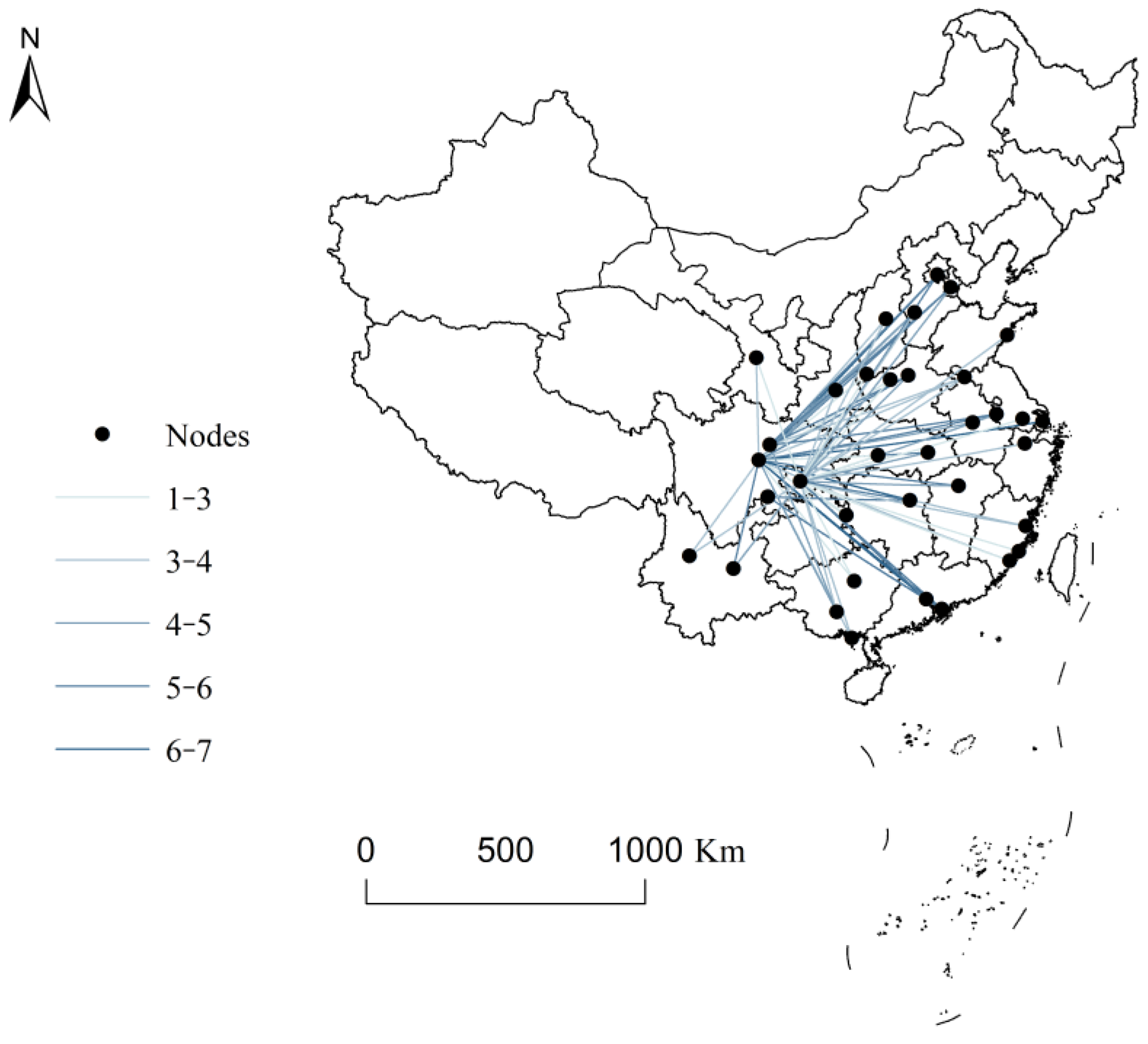
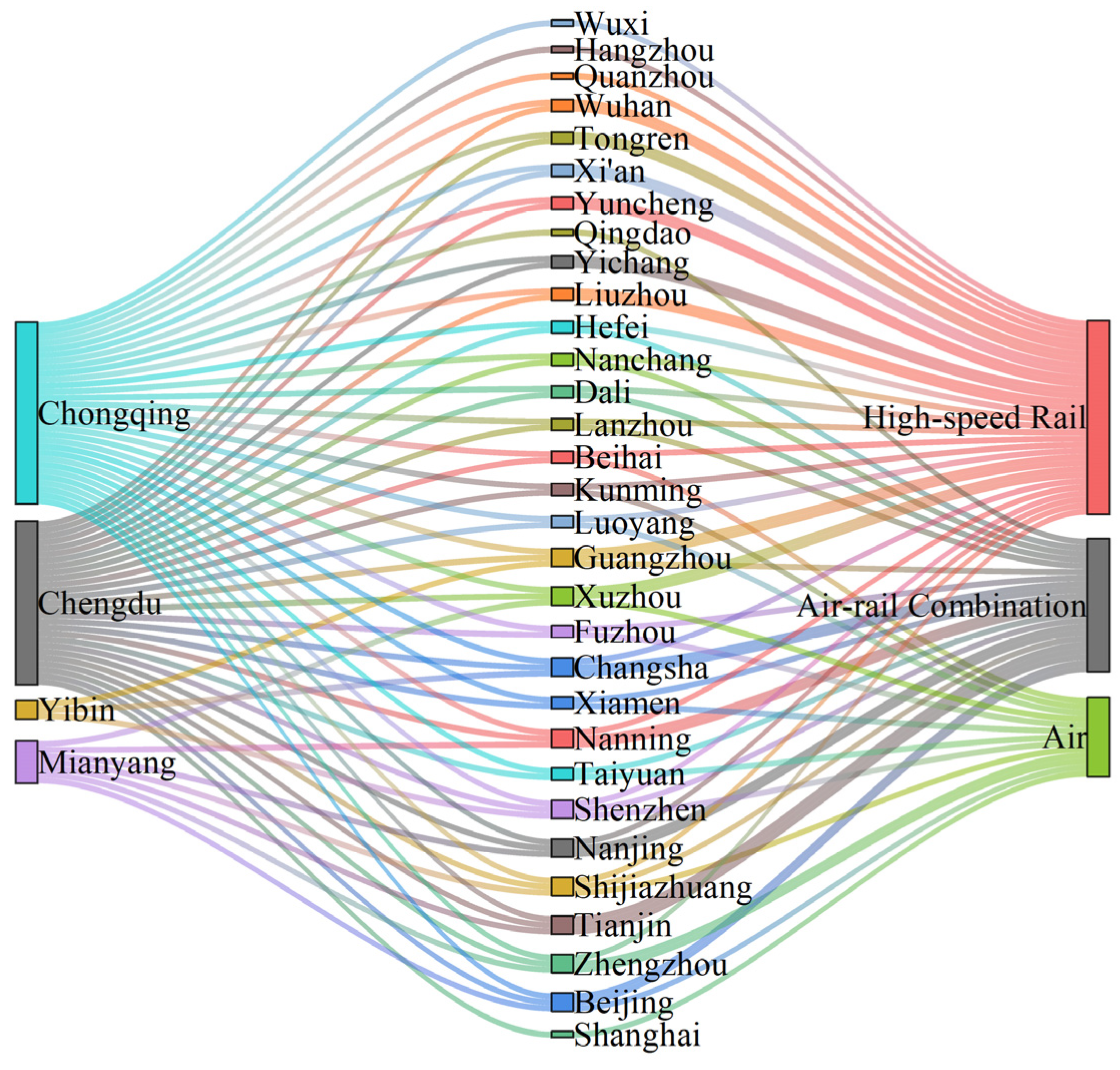
  • In the travel network of the Chengdu–Chongqing economic circle, 47.8% of the total number of passengers chose high-speed rail for direct travel. Under the air–rail combination travel scenario, Chengdu and Yibin have relatively obvious hub characteristics.
  • The conducted ridge regression analysis found that comfort had the greatest impact on the probability of passengers choosing air direct. Convenience had the greatest impact on the probability of choosing high-speed rail direct, which was slightly higher than the probability of choosing air direct. Passengers were least inclined toward choose HA travel when the ticket’s price increased, while the impact on the probability of choosing air direct was relatively small.
  • By means of sensitivity analyses, it was found that the factors that constitute the generalized cost have certain differences in the impact of passengers’ choice behavior. Fatigue recovery times were not sufficiently flexible for passengers to choose their travel mode, while the travel time and per capita time value of the main traffic are flexible for passengers to choose their travel modes. At the same time, the sensitivity of the three factors relative to a passenger’s travel choice ranked from high-speed rail direct, air–rail combined travel, and air direct.
In view of this, the travel selection behavior of passengers can effectively reflect the rationality of the current market layout of different transport networks. For air–rail intermodal transport products with potential within the medium- and long-distance transportation market, different transport enterprises should strengthen cooperation between transport modes to meet the travel demand of passengers and maximize the utilization of resources. Meanwhile, transport companies should consider ticket price, quickness, convenience, comfort, and other factors to design different types of products for the convenience of travelers. Finally, different transport enterprises should reasonably evaluate the preference of passengers in choosing paths, appropriately improving the relatively lacking transport service attributes, changing the strategic layout of passenger transport routes with relatively weak advantages, and seeking other passenger transport markets with potential advantages to implement the development concept that includes changing from a focus on quantity to a focus on high quality products. This paper provides a research perspective on passenger transport selection behavior, which plays a certain role in the reasonable discrimination of the current advantages of different transport enterprises. In subsequent research studies, the corresponding assignment model will be introduced to provide strategic references for the transportation enterprises’ shift delivery and network planning.

Author Contributions

Conceptualization, P.Z. and W.Z.; data curation, P.Z.; formal analysis, P.Z. and W.Z.; investigation, L.Z.; methodology, W.Z.; resources, H.S.; software, R.D.; validation, W.Z.; writing—original draft, W.Z. and R.D.; writing—review and editing, W.Z. and R.D. All authors have read and agreed to the published version of the manuscript.

Funding

This research was funded by National Natural Science Foundation of China: grant number U2033213 and U1733127. It was also funded by the Civil Aviation Flight Technology and Flight Safety Research Base Project, grant number F2019KF03; by the National College Students Innovation and Entrepreneurship Training Program, grant number S202110624027; and the Civil Aviation Management Science and Engineering Research Institute, grant number JG2022-24.

Institutional Review Board Statement

Not applicable.

Informed Consent Statement

Not applicable.

Data Availability Statement

The data used to support the findings of this study are available from the corresponding author upon request.

Conflicts of Interest

The authors declare no conflict of interest.

References

  1. Gi, K.; Sano, F.; Akimoto, K. Bottom-up Development of Passenger Travel Demand Scenarios in Japan Considering Heterogeneous Actors and Reflecting a Narrative of Future Socioeconomic Change. Futures 2020, 120, 102553. [Google Scholar] [CrossRef]
  2. Chai, J.; Zhou, Y.; Zhou, X.; Wang, S.; Zhang, Z.G.; Liu, Z. Analysis on Shock Effect of China’s High-Speed Railway on Aviation Transport. Transp. Res. Pt. A-Policy Pract. 2018, 108, 35–44. [Google Scholar] [CrossRef]
  3. Li, Z.-C.; Sheng, D. Forecasting Passenger Travel Demand for Air and High-Speed Rail Integration Service: A Case Study of Beijing-Guangzhou Corridor, China. Transp. Res. Pt. A-Policy Pract. 2016, 94, 397–410. [Google Scholar] [CrossRef]
  4. Wang, Y.; Sun, L.; Teunter, R.H.; Wu, J.; Hua, G. Effects of Introducing Low-Cost High-Speed Rail on Air-Rail Competition: Modelling and Numerical Analysis for Paris-Marseille. Transp. Policy 2020, 99, 145–162. [Google Scholar] [CrossRef]
  5. Sun, X.; Zhang, Y.; Wandelt, S. Air Transport versus High-Speed Rail: An Overview and Research Agenda. J. Adv. Transp. 2017, 2017, e8426926. [Google Scholar] [CrossRef] [Green Version]
  6. Pagliara, F.; Vassallo, J.M.; Román, C. High-Speed Rail versus Air Transportation: Case Study of Madrid–Barcelona, Spain. Transp. Res. Record 2012, 2289, 10–17. [Google Scholar] [CrossRef] [Green Version]
  7. Yamín, D.; Medaglia, A.L.; Prakash, A.A. Exact Bidirectional Algorithm for the Least Expected Travel-Time Path Problem on Stochastic and Time-Dependent Networks. Comput. Oper. Res. 2022, 141, 105671. [Google Scholar] [CrossRef]
  8. Hu, J.; Yang, B.; Guo, C.; Jensen, C.S. Risk-Aware Path Selection with Time-Varying, Uncertain Travel Costs: A Time Series Approach. VLDB J. 2018, 27, 179–200. [Google Scholar] [CrossRef]
  9. Feng, Y.; Zhao, J.; Sun, H.; Wu, J.; Gao, Z. Choices of Intercity Multimodal Passenger Travel Modes. Physica A 2022, 600, 127500. [Google Scholar] [CrossRef]
  10. Wang, Y.; Yan, X.; Zhou, Y.; Xue, Q. Influencing Mechanism of Potential Factors on Passengers’ Long-Distance Travel Mode Choices Based on Structural Equation Modeling. Sustainability 2017, 9, 1943. [Google Scholar] [CrossRef]
  11. Wang, J.; Jiao, J.; Du, C.; Hu, H. Competition of Spatial Service Hinterlands between High-Speed Rail and Air Transport in China: Present and Future Trends. J. Geogr. Sci. 2015, 25, 1137–1152. [Google Scholar] [CrossRef]
  12. Cadarso, L.; Vaze, V.; Barnhart, C.; Marín, Á. Integrated Airline Scheduling: Considering Competition Effects and the Entry of the High Speed Rail. Transp. Sci. 2017, 51, 132–154. [Google Scholar] [CrossRef]
  13. Su, M.; Luan, W.; Yuan, L.; Zhang, R.; Zhang, Z. Sustainability Development of High-Speed Rail and Airline—Understanding Passengers’ Preferences: A Case Study of the Beijing–Shanghai Corridor. Sustainability 2019, 11, 1352. [Google Scholar] [CrossRef] [Green Version]
  14. Li, Y.-T.; Schmöcker, J.-D. Adaptation Patterns to High Speed Rail Usage in Taiwan and China. Transportation 2017, 44, 807–830. [Google Scholar] [CrossRef]
  15. Li, X.; Li, X.; Li, X.; Qiu, H. Multi-Agent Fare Optimization Model of Two Modes Problem and Its Analysis Based on Edge of Chaos. Physica A 2017, 469, 405–419. [Google Scholar] [CrossRef]
  16. Ruiz-Rúa, A.; Palacín, R. Towards a Liberalised European High Speed Railway Sector: Analysis and Modelling of Competition Using Game Theory. Eur. Transp. Res. Rev. 2013, 5, 53–63. [Google Scholar] [CrossRef] [Green Version]
  17. Zhang, A.; Wan, Y.; Yang, H. Impacts of High-Speed Rail on Airlines, Airports and Regional Economies: A Survey of Recent Research. Transp. Policy 2019, 81, A1–A19. [Google Scholar] [CrossRef]
  18. Pan, C.; Wang, H.; Guo, H.; Pan, H. How Do the Population Structure Changes of China Affect Carbon Emissions? An Empirical Study Based on Ridge Regression Analysis. Sustainability 2021, 13, 3319. [Google Scholar] [CrossRef]
  19. İmre, Ş.; Çelebi, D. Measuring Comfort in Public Transport: A Case Study for İstanbul. Transp. Res. Procedia 2017, 25, 2441–2449. [Google Scholar] [CrossRef]
  20. Du, M.; Chen, A. Sensitivity Analysis for Transit Equilibrium Assignment and Applications to Uncertainty Analysis. Transp. Res. Pt. B-Methodol. 2022, 157, 175–202. [Google Scholar] [CrossRef]
Figure 1. Passenger travel path scenarios.
Sustainability 15 00636 g001
Figure 2. The spatial layout of outbound travel routes of passengers in the Chengdu–Chongqing economic circle. The lines (edges) in the figure represent the external travel routes of the Chengdu–Chongqing economic circle. The weight on the edges is the number of travel paths (transportation modes) that passengers can choose from. Natural discontinuous grading is adopted. When the lines are darker, there are more travel paths for passengers to choose from.
Sustainability 15 00636 g002
Figure 3. Passengers’ travel preference for different OD connections. The left side of the figure shows a city node with three travel paths in the Chengdu–Chongqing economic circle. If the grid is longer, then there are more OD pairs taking this node as the starting point. The middle column is the travel destination outside the system, and the rightmost column is the transportation mode of the optimal travel path on each OD pair. The longer the square, the higher the proportion of passengers who choose this transportation mode to travel.
Sustainability 15 00636 g003
Figure 4. The ridge traces of the air transport mode.
Sustainability 15 00636 g004
Figure 5. R-SQUARE vs. ϑ of the air transport mode.
Sustainability 15 00636 g005
Table 1. Multicollinearity test result.
VariableAHHA
VIFVIFVIF
lnE1.412.241.02
lnQ33.4270.3870.74
lnF20.777.755.87
lnC54.8944.1154.35
Mean VIF27.6231.1233.00
Table 2. Ridge regression result.
VariableCoefficientStandard
Error
Standard
Coefficient
t-StatisticSig.t
lnE−0.2240.017−0.221−13.0130.001
lnQ0.2350.0150.23115.6310.001
lnF0.2390.0150.23515.6800.001
lnC0.2430.0160.24015.0670.001
Constant−0.3701.5070.000−0.2450.001
Note: R = 0.994; R2 = 0.988; F = 61.787; Sig.(F) = 0.003.
Table 3. Ridge regression results.
VariableAHHA
CoefficientStd. ErrorCoefficientStd. ErrorCoefficientStd. Error
ln E−0.224 ***0.017−0.230 ***0.016−0.312 ***0.047
ln Q0.235 ***0.0150.233 ***0.0160.061 ***0.022
ln F0.239 ***0.0150.242 ***0.017−0.0360.056
ln C0.243 ***0.0160.240 ***0.0160.095 ***0.024
Constant−0.370 ***1.507−0.747 *1.5850.4330.407
Note: *** and * indicate significance at the levels of 1% and 10%, respectively.
Table 4. Calculation results of fatigue recovery time.
ModesFatigue Recovery Time
ParameterAveragetElastic
High-speed rail−0.5341.751−5.0980.615
Air0.2490.3562.0740.061
Air–rail0.3650.5493.1590.134
Table 5. Calculation results of travel time.
ModesTravel Time
ParameterAveragetElastic
High-speed rail−0.6408.189−6.7123.394
Air0.2522.0452.1000.356
Air–rail0.4073.7143.5951.008
Table 6. Calculation results of the per capita time value.
ModesPer Capita Time Value
ParameterAveragetElastic
High-speed rail−0.39048.325−3.42012.049
Air0.25248.3252.1008.402
Air–rail0.26148.3252.1808.460
Disclaimer/Publisher’s Note: The statements, opinions and data contained in all publications are solely those of the individual author(s) and contributor(s) and not of MDPI and/or the editor(s). MDPI and/or the editor(s) disclaim responsibility for any injury to people or property resulting from any ideas, methods, instructions or products referred to in the content.

