Article

Exploring Farmers’ Expectation toward Farm-Gate Price of Rice in Japan by Positive Mathematical Programming

by
Takahiro Nakashima
1,* and
Shoko Ishikawa
2
1
Strategic Planning Headquarters, National Agriculture and Food Research Organization (NARO), 3-1-3 Kannondai, Tsukuba 305-8604, Ibaraki, Japan
2
Central Region Agricultural Research Center, NARO, 2-1-18 Kannondai, Tsukuba 305-8666, Ibaraki, Japan
*
Author to whom correspondence should be addressed.
Sustainability 2023, 15(1), 621; https://doi.org/10.3390/su15010621
Submission received: 22 November 2022 / Revised: 22 December 2022 / Accepted: 23 December 2022 / Published: 29 December 2022

Abstract

:
Positive mathematical programming (PMP) has a substantial number of applications in the field of agricultural and resource economics. Their focus has often been placed on the simulation analysis of farmers’ response to drastic changes in exogenous factors especially brought about by policy changes. In the present study, an exploration was made to widen the application area of the PMP approach, targeting farmers’ expectation toward the farm-gate price of rice in comparison with that of wheat under the policy to suppress overproduction. When domestic consumption is mature and the regulation of production by the government is present, farmers’ expectation toward the farm-gate price of a crop can be assumed to fall in response to an increased allocation of land area to produce the crop. The degree of the fall is defined as the expectation fall index (EFI) in the present study. A proposition was made as to the procedure for quantifying EFI using the PMP approach with statistical datasets of multiple years retrieved from the Ministry of Agriculture, Forestry, and Fisheries. The present study is considered to have provided a basis to discuss the formation processes of farmers’ attitudes toward policy measures.

1. Introduction

Overwhelmed by the image of a highly industrial society, it may not be known to the world that Japan is a country that is capable of feeding the mouths of a more than 120 million population with a staple food (i.e., rice). It would be even fewer people who know that wheat and soybean are often grown on behalf of rice in paddies in Japan.
After successful recovery from serious food shortage in the postwar era, Japanese rice production recorded as high as 18.9 million tons in the 1960s [1]. Ironically, simultaneous industrialization was successful enough to diminish the national dream of eating rice every meal rather quickly, as people started consuming foods other than rice, especially meat [2,3,4]. This was during the time when the policy, the acreage control program, was installed with the intention to reduce domestic rice production [5]. Since 1969, farmers have been encouraged to grow crops such as wheat, soybean, and vegetables instead of rice [6] (pp. 63–66). Unlike profitable vegetables, wheat and soybean had to be heavily subsidized [7,8] (pp. 5–13). In other words, no farmers in Japan were willing to grow wheat and soybean in paddies unless they were subsidized.
Apart from exceptionally strong exporters of agricultural commodities represented by Australia and New Zealand, many nations employ a variety of measures to protect their agriculture [9,10], of which the Common Agricultural Policy by the European Union is one [6] (pp. 59–60) [11] (pp. 216–217). Policies similar to the acreage control program in Japan have also been introduced by the South Korean and Taiwanese governments [12,13,14]. The acreage control program was successful in suppressing the amount of rice produced in Japan [8] (pp. 6–7). The paddy area assigned to rice was reduced by 43% from 2.70 million hectares (ha) in 1971 to 1.54 million ha in 2019 [1]. One thing the successful looking policy did not tell us was how farmers perceived the series of measures derived from the acreage control program itself.
Positive mathematical programming (PMP) has a substantial number of applications in the field of agricultural and resource economics [15,16,17,18,19]. Their focus has almost always been placed on the simulation analysis of farmers’ responses to drastic changes in exogenous factors especially brought about by policy measures [20,21], while paying less attention to farmers’ perception toward policy measures. It is vital to understand farmers’ perception of the existing policy measures in order to realize a sustainable and food-secured society. The PMP approach may be able to play a role in enhancing communication, though non-interactive, between farmers and policymakers. Farmers’ expectation toward farm-gate prices can be regarded as reflecting how farmers see and experience their situations as influenced by the current agricultural policies. Thanks to the detailed information that was made available to the public by the Ministry of Agriculture, Forestry, and Fisheries (MAFF) as to subsidy payments from 2011 onward in Japan, the environment in which to apply the PMP approach to the subject has been prepared.
The objective of the present study was therefore to apply the PMP approach to farmers’ expectation toward the farm-gate price of rice in comparison with that of wheat under the acreage control program. When domestic consumption is mature and the regulation of production by the government is present, farmers’ expectation toward the farm-gate price of a crop can be assumed to fall in response to an increased allocation of land area to produce the crop. The degree of the fall here was defined as the expectation fall index (EFI) in the present study. It is the process of the quantification of EFI where the merit of the PMP approach is explored. In the Materials and Methods section, a procedure to calculate the EFI using a PMP-based regional crop production model was established. The calculated EFI values under conditions differing in crop, farm scale, and region were subjected to analysis of variance and are presented in the Results. Finally, in the Discussion, the implication for future policy is discussed based on the results.

2. Materials and Methods

EFI was quantified for each crop using a PMP-based regional crop production model.

2.1. Model

In the PMP-based model, farmers expect the farm-gate price of a given crop to fall linearly in response to an increase in land area allocated to the crop. The farm-gate price here includes the subsidy provided by the government. Furthermore, it was assumed that farmers cannot influence the prices of purchasable inputs such as fertilizers and pesticides. Additionally, farmers are to pursue the maximization of the expected profit at a regional scale under two resource constraints (i.e., cultivatable acreage and labor hours). The upper limit of the former is regulated on a regional basis. The regional crop production model is formulated as a quadratic programming (QP) model (see Table 1 for the definitions of the variables and parameters):
max x 1 , ,   x n   π Q P = i = 1 n [ p i ( x i ) y i c i ] x i N F i
p i ( x i ) = d i 0.5 q i x i
  s . t .   i = 1 n x i N F i b 0
l i x i b i
x i 0
where the parameters y i , c i , N F i , l i , b 0 , and b i are specified based on the statistical dataset described in the latter part of this section, while the parameters d i and q i are to be calibrated. Following the assumption described above, the parameter d i must be greater than zero and the parameter q i must be either greater than or equal to zero.
EFI was defined in the present study by
E F I i = d p i ( x i * ) d x i   x i * p i ( x i * )
where the asterisk indicates that the variable is evaluated at the optimum solution. EFI is the index to quantify the percentage by which farmers’ expectation toward the farm-gate price falls in response to an increase in land area allocated to the crop by one percent. The assumption d p i ( x i ) / d x i 0 gives E F I i 0 . The minimum value of EFI is zero and the maximum value does not exceed one (see Appendix A). Zero EFI indicates that farmers expect the farm-gate price to be independent of their decision making on the land area allocated to the crop. This can happen when farmers face a perfectly competitive crop market without intervention. Otherwise, EFI takes a positive value. A greater EFI indicates that farmers expect the farm-gate price to drop greatly. In other words, they receive less incentive to increase the land area allocated to the crop in question.
As a situation to make EFI great, one can imagine a crop, a large part of whose farm-gate price consists of the subsidy payment by the government. Wheat falls in this category, with the percentage of subsidy payment to the farm-gate price (hereafter the subsidy rate) exceeding 70% on average [22] (Table A1 in Appendix B). Because subsidies are budgetarily constrained, few farmers would increase the production area knowing that subsidies are not likely to cover the grain obtained from the additional acreages. Namely, the EFI would rise with increasing subsidy rates. As for rice, the subsidy rate is basically low and does not exceed 10% (Table A1). It is therefore postulated, as a first working hypothesis in the present study, that the EFI of wheat is greater than that of rice. Additionally, as shown in Equation (6), the EFI is calculated by dividing the rate of the expected price change by the rate of acreage change. This means that the change in acreage itself increases with the farm scale. Thus, it was assumed as a second working hypothesis in the present study that the EFI of rice increases with the farm scale. Focus was placed on rice in the second hypothesis, intending to discuss the impacts of the acreage control program on rice production by showing some key arguments held in Japan. In order to help readers follow the present study, a piece of information is provided that the rate of restriction is uniform irrespective of the farm scale as to the acreage control program [23,24].

2.2. Calibration Procedure

For the calibration of d i and q i , standard PMP prepares the following LP model [25]:
max x 1 , , x n   π L P = i = 1 n ( p i y i c i ) x i N F i
s . t .   Equations (3)–(5) and
x i x i o b s + ε i [ ρ i ]
where p i is a parameter that is specified on the basis of statistical data as well as y i , c i , N F i , l i , b 0 , and b i . x i o b s is the observed value of x i in the base year, and ε i is a positive number close to zero. Equation (8) prevents x i from exceeding x i o b s . The dual variable associated with Equation (8) is expressed as ρ i . The dual variable ρ i is an indicator of whether the LP model without Equation (8) reproduces the observed value of the primal variable as the result of optimization. Unless the optimum value ρ i * is zero for all i , the LP model (3)–(5), (7) is interpreted as “false”. This is because the LP model (3)–(5), (7) deviates from the observed land allocation. PMP attributes the deviation, measured by ρ i , of the LP model (3)–(5), (7) to a misspecification of the objective function. The misspecification is reflected in “true” objective function, which is nonlinear in variables. Equation (2) enables the nonlinearization of the objective function in the present study.
Given that the optimum dual variables associated with Equations (3) and (4) coincide with both the QP model (1)–(5) and the LP model (3)–(5), (7), (8), the necessary conditions for optimizing the models derive linear equations of d i and q i :
p i y i N F i ρ i = d i y i N F i q i x i o b s y i N F i
Equation (9) indicates how the parameters d i and q i should be calibrated so that the QP model (1)–(5) exactly reproduces the observed land allocation in the base year. However, a unique solution could not be found for Equation (9) with respect to the unknown parameters d i and q i , unless additional information were supplied [15,16]. As known as an ill-posed problem [26], many combinations of the parameters d i and q i can satisfy Equation (9). The theoretical feature that any combination satisfying Equation (9) reaches the identical solution in the base year does not guarantee the same phenomena occurring in cropping years other than the base year [15,16].

2.3. Selecting Calibration Methods

The calibration method employed in the present study followed the procedure previously published [17,27]. Decomposition of Equation (9) gives Equations (10) and (11).
d i = s p i t ρ i * y i N F i  
q i = ( 1 s )   p i y i N F i ( 1 t ) ρ i * y i N F i x i o b s  
where s and t , respectively, denote the allocation rates of p i y i N F i   and ρ i to d i y i N F i in Equation (9). Because Equations (10) and (11) satisfy Equation (9), a feasible set of ( s , t ) corresponds to a calibration method of the parameters d i and q i , which satisfies Equation (9). This s t or two-parameter approach can be postulated as an extension of the original approach [28]. The extended version has the strength already described in the previous work [27].
In the present study, a square was defined so that 1 s 2 and 1 t 0 . The points located on the grids inside the square as well as the square sizes were the target of the examination. The employment of grid spacing of 0.1 from the origin both in the s and t axes resulted in 121 sets of ( s , t ) , from which the same number of calibration methods were generated. For example, consider the set ( s , t ) = ( 1 , 1 ) as Point A. Point A leads to the calibration method d i = p i + ρ i * / y i N F i and q i = 2 ρ i * / y i N F i x i o b s . This calibration method ensures the accurate reproduction of the observed levels of the farm-gate price and profit for each production process as well as the observed land-area allocation in the base year [17,19]. Point A was set as baseline in the present study.
For each set of   s   and   t , the parameters d i and q i were calculated in the base year, and the QP model (1)–(5) was optimized using the parameter values of y i , c i , N F i , l i , b 0 , and b i in multiple cropping years including the base year. The best combination of s and t was considered to make percentage absolute deviation (PAD) minimum for the multiple cropping years. PAD was calculated in two directions between the observed and the optimum land allocation and between the observed and the simulated crop price:
P A D l a n d   = 1 m j = 1 m i = 1 n w i j | x i j * x i j o b s | x i j o b s × 100
P A D p r i c e = 1 m j = 1 m i = 1 n w i j | d i 0.5 q i x i j * p i j | p i j × 100
where j stands for the cropping year and w i j is the weighing factor, w i j = N F i j / i = 1 n N F i j to calculate the regional value. The mean of P A D l a n d   and P A D p r i c e was calculated as
P A D m e a n = 0.5 ( P A D l a n d + P A D p r i c e )
The set of ( s , t ) that minimizes P A D m e a n was selected to determine the most suitable calibration method. For the references, P A D l a n d   , P A D p r i c e , and P A D m e a n were evaluated only in the base year and referred to as P A D l a n d b a s e , P A D p r i c e b a s e , and P A D m e a n b a s e , respectively.

2.4. Dataset

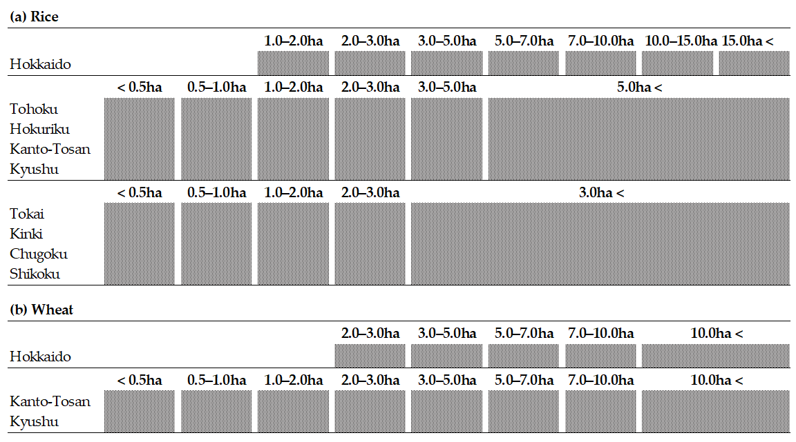
The procedure to select the calibration methods was applied to nine regions for rice and three regions for wheat (Figure 1). The data series sorted for farm scales (Figure A1) were obtained from the Production Costs for Rice and Wheat (Farm Households) between 2011 and 2018 [22]. Possible combinations by matching regions and years were 72 and 24 datasets for rice and wheat, respectively, where nine and two combinations had to be treated as missing values for the former and the latter.
The detailed explanations for p i j , y i j , c i j , f i j , l i j , b 0 j , b i j , and x i j o b s are described below.
p i j : Farm-gate price including the subsidy of the crop for each year in Japanese Yen per kilograms (Yen kg–1), where the price for each crop is calculated by dividing revenues from production by the quantity of crop supplied;
y i j : Yield of crop per unit area (in kg ha–1);
c i j : Sum of the variable cost, in Yen ha–1, for purchasable inputs of seed, fertilizers, agricultural chemicals, electricity and fuels, and other materials per unit area;
N F i j : Number of surveyed farms;
l i j : Annual labor hours required for crop production per unit area (in h ha–1);
b 0 j : Sum of the observed land use area for crop production (ha);
b i j : Labor hour constraint for crop production per year (h);
x i j o b s : Observed land area allocation to crop production (ha);
The QP model (1)–(5) was calibrated setting the dataset of the latest year as the base year and evaluated using all the available datasets irrespective of crop and region. For the numerical computation, the General Algebraic Modeling System (GAMS) version 27.2 was used.

2.5. Calculation of EFI and Statistical Analysis

Once the parameters d i and q i were calibrated, the EFI was calculated by Equation (15) derived from Equations (2) and (6):
E F I i j = 0.5 q i x i j * d i 0.5 q i x i j *
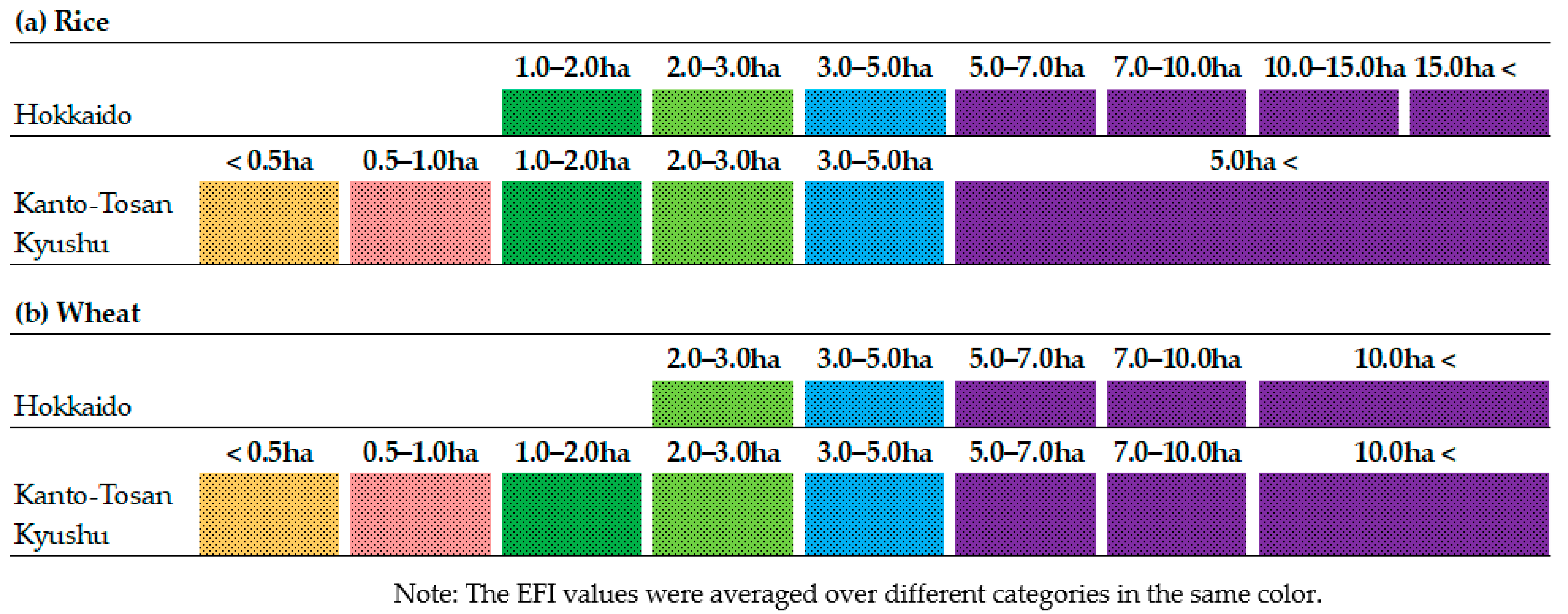
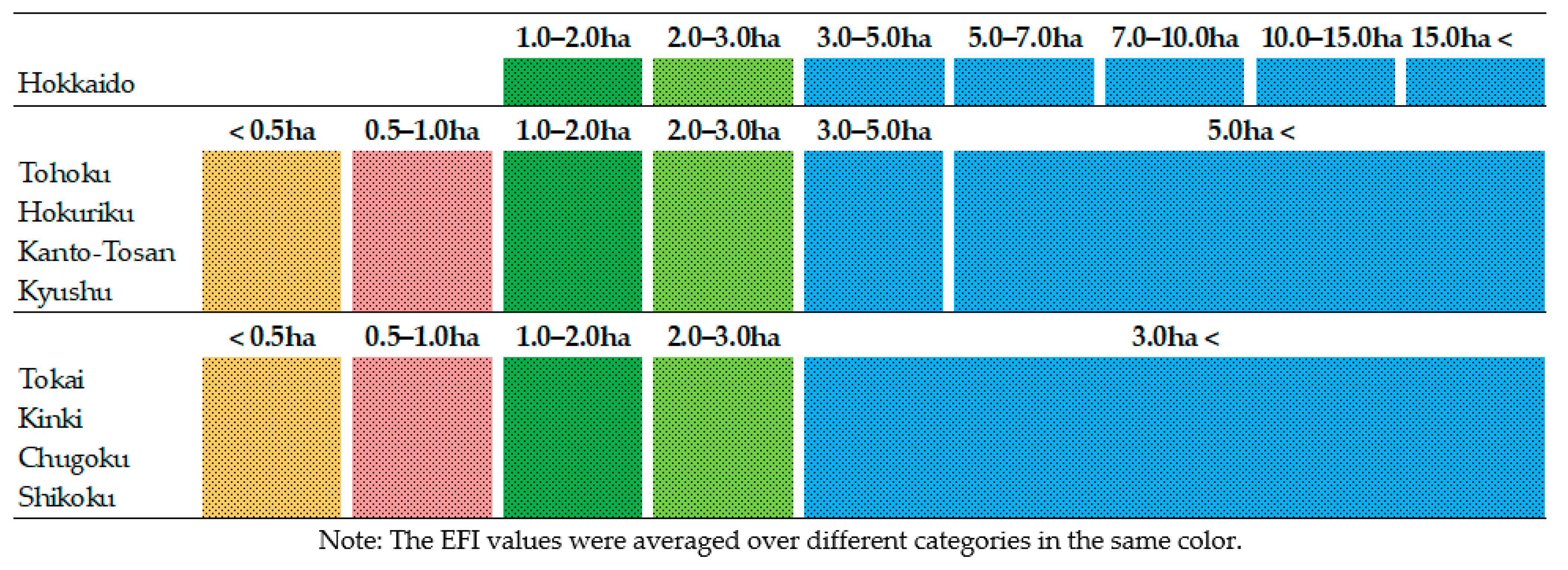
where i and j denote the farm scale category and cropping year, respectively. Calculated values of EFI were subjected to statistical analysis. Analysis of variance (ANOVA) and multiple comparisons with the Scheffé method were performed to test two hypotheses related to the working hypotheses described in Section 2.1. Hypothesis 1, derived from the first working hypothesis, is that neither crops nor regions affect EFI. Hypothesis 2, derived from the second working hypothesis, is that neither the farm scales nor regions affect the EFI of rice. The dataset to test Hypothesis 1 included only three regions (the Hokkaido, Kanto-Tosan, and Kyushu regions) due to the data availability related to wheat (Figure A2). The dataset to test Hypothesis 2 included nine regions (Figure A3). The SPSS statistical program version 28 (IBM) was used to analyze the results. All significant results are referred to at the 5% level unless otherwise specified.

3. Results

3.1. Selected Calibration Methods and Model Evaluation

The QP model (1)–(5) was applied to target crops in the base year. The computed results of rice in the Hokkaido region are presented in Figure 2, which consists of P A D l a n d b a s e , P A D p r i c e b a s e , and P A D m e a n b a s e . The computed value of P A D l a n d b a s e was equal to zero irrespective of ( s , t ) (Figure 2a), while that of P A D p r i c e b a s e was equal to zero only at Point A, ( s , t ) = ( 1 , 1 ) (Figure 2b). This indicates that only the calibration method corresponding to Point A made the QP model (1)–(5) accurately reproduce the observed levels of farm-gate prices as well as the observed land allocation in the base year. This result was also supported by the observation that the computed values of P A D m e a n b a s e were the smallest and equal to zero at Point A (Figure 2c). This performance of the benchmark case in the base year was confirmed in all regions and crops considered in the present study and are therefore not presented.
Corresponding to the base year in Figure 2, the results of the multiple cropping years are presented in Figure 3. The computed values of P A D l a n d and P A D p r i c e were 2.6% and 13.9% at Point A (Figure 3a,b). Unlike the base year alone, the values were neither zero nor the smallest. The computed value of P A D m e a n was 8.3% at Point A (Figure 3c). This was 40th from the smallest value of P A D m e a n out of the 121 sets of ( s , t ) described in Section 2.3. The smallest value of P A D m e a n was explored from the 40 sets of ( s , t ) colored in pink in Figure 3c. This was obtained at Point B, ( s ,   t ) = ( 1.4 , 0.2 ) (Figure 3c). At Point B, the computed value of P A D m e a n was 5.4%, which was smaller by 2.9 percentage points than the value at Point A (Figure 3c). Point B was selected to calibrate the QP model (1)–(5) for the rice case in the Hokkaido region.
The rest of the results are summarized in Table 2. The minimum value of P A D m e a n was, in most regions, less than 10% or even less than 5%. Two cases (rice in the Kanto-Tosan and the Tokai regions) where P A D m e a n exceeded 10% stayed within the practical threshold of 15% [29] (p. 271). Therefore, the calibration methods were successfully selected in the present study.

3.2. EFI and ANOVA Results

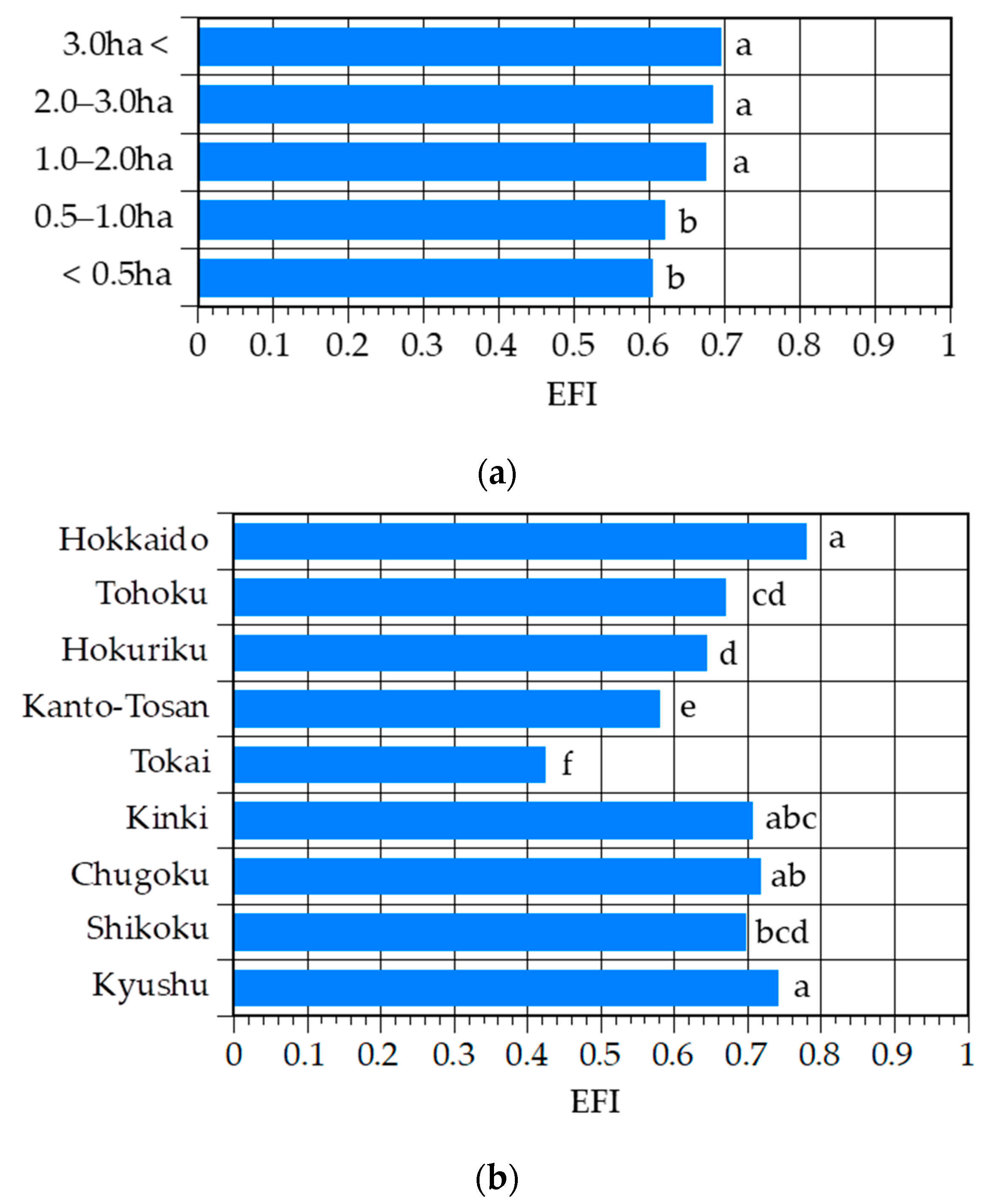
Table 3 presents the ANOVA results of the EFI for two hypotheses, Hypothesis 1 and 2. As to the former, there was a significant interaction between crops and regions ( p < 0.001 ). As shown in Figure 4, the EFI was greater for wheat than for rice in the Kanto-Tosan region, which was in accordance with the first working hypothesis described in Section 2.1. This, however, did not hold for the Hokkaido and the Kyushu regions, which was against the initial postulation. Thus, one cannot say that the EFI of wheat is greater than that of rice. The estimated EFI value of rice was 0.78, 0.58, and 0.74 in the Hokkaido, the Kanto-Tosan, and the Kyushu regions, respectively, and that of wheat was 0.69, 0.76 and 0.69, correspondingly. It was 0.70 when averaged over rice and wheat. Regarding the latter hypothesis, no interaction was observed between the farm scales and regions (Table 3). The EFI was significantly affected by the farm scales ( p < 0.001 ) and by regions ( p < 0.001 ). As displayed in Figure 5a, EFI was significantly greater for the farm scale above 1 ha than for that below 1 ha ( p < 0.001 ). Contrary to the first working hypothesis, the outcome of the second working hypothesis was in accordance with the initial expectation. Figure 5b shows that the regions showing especially greater EFI were the Hokkaido and the Kyushu regions. The Kanto-Tosan and the Tokai regions showed significantly smaller EFI than any other region.

4. Discussion

In the present study, an exploration was made to widen the application area of the PMP approach. The attempt successfully quantified, through indexing, farmers’ expectation toward the farm-gate prices of rice and wheat under the acreage control program. The reason why we did not employ a more popular econometric approach [30,31] is because it is not necessarily good at treating the targets of policies [15,16]. The merit of applying the PMP approach to this subject can be summarized as the explicit inclusion of the target of a policy of interest. In the present study, the land-area constraint in Equation (3) was the target of the acreage control program. By employing the recently proposed method [27] instead of standard econometric estimation methods, it became possible to provide a basis to discuss the formation processes of farmers’ attitudes toward the policy measures. It can therefore be deduced from the present study that the PMP approach has the potential to reveal farmers’ perceptions of the policy measures in other countries.
Considering that the EFI takes a value between zero and one (Appendix A), the EFI of 0.70 observed in the present study was large. This can be interpreted that farmers receive little incentive to expand the production area allocated to rice and wheat. This also suggests that PMP studies assuming the EFI to be zero are overly optimistic about farmers’ expectation toward farm-gate prices under the current policy in Japan. The reason for poor motivation to grow wheat can be speculated rather easily. Subsidies to form a large part of the income for wheat (exceeding 70% on average, Table A1) are budgetary constrained, as indicated in Section 2.1. Interestingly, the EFI of rice was comparable to or even greater than that of wheat in the Hokkaido and the Kyushu regions (Figure 4). In other words, farmers have less incentive to produce rice. This is contrast to our initial view. What lies behind the poor motivation? Is the tiny subsidy rate bound to rice, roughly one-tenth of that of wheat (Table A1), not a guarantee for farmers to act according to the market forces?
The answer to this question could be found in the history back in 1969 when the acreage control program was installed. As is often the case with paddy-based rural areas, a single decision to represent the community must be made. Common infrastructure to form the foundation of a paddy-based community, especially irrigation facilities, would not allow an individual farmer to pursue his/her own benefit by paying little attention to neighbors [7,32,33]. Rural communities based on other grains such as wheat and maize may be influenced by drying and storing facilities that are regarded as common infrastructure. The magnitude of the impact of water-related facilities to paddy communities, however, is even greater. Therefore, farmers are inevitably influenced by the will of the community. In addition, a cooperative attitude to communities, often told as a virtue of the Japanese, could turn into obedience to authority [8] (pp. 12–13). This virtue could strengthen a once-established, so to speak, bureaucratic system, even if it were not fit for the times. The participation to the acreage control program was conducted on a voluntary basis. However, one can imagine that it is not very easy for a single farmer to go against the will of the community. With the domestic rice consumption continuing to slump, it is not surprising that the EFI has remained high. The relatively low EFI observed in the Kanto-Tosan region (Figure 4), which includes the Tokyo metropolitan area, Japan’s largest consumer area, may support this view.
Over 50 years of history of the policy, a uniformly imposed rate of restriction on farms, irrespective of scale, as mentioned in Section 2.1, has particularly been a target of criticism. A view that the uniform rate of restriction has been a cause of provoking farmers to harbor ill-feeling against the policy is in line with the majority view of agricultural economists in Japan, who are concerned that large-scale farmers could possibly be discouraged by the restricting policy imposed at the uniform rate [23,24,34,35]. The present study verified the established view from farmers’ price expectation toward the farm-gate price of rice, implying that larger farmers have been affected more by the policy. It should be noted that the recent advent of megafarms or corporative farms over 100 ha was out of the scope of the present study. Apparently, the EFI differed more greatly among regions (Figure 5), suggesting that farmers’ willingness to increase their acreage may be influenced by geographic locations. In other words, farmers in some regions may have experienced the impacts of the policy more strongly than those in other regions, which has been going unnoticed.
The consequence of joining in the acreage control program was, however, probably not felt to be damaging due to the successful industrialization, which created abundant employment in the 1970s. A younger generation of farm household was employed, providing off-farm income to the household, while their parents and grandparents kept being engaged in agriculture [6] (pp. 83–89) [8] (pp. 16–19). Agricultural mechanization, supported by off-farm income, advanced quickly in this environment. According to the agricultural census [36], part-time farm households accounted for 86% of total farm households in 1985. The collapse of Japan’s “bubble economy” in the early 1990s, followed by the long-lasting deflation, was experienced as a deteriorated environment in seeking employment in rural areas. This weakened the precondition to support the structure of rural areas that relied on off-farm income. It is not surprising that the pandemic of COVID-19 made the situation even worse [37,38]. The year 2019 is recalled as a year when the agricultural sector in the world was challenged by a number of hardships such as supply chain disruption by the pandemic, occurrences of floods, and locust attacks [39,40,41,42]. In Japan, impacts of these events might have been felt by vulnerable population groups as deteriorated community functions, considering that the suicide rates worryingly increased, especially among females and children and adolescents from July to October in 2020 [38].
Looking at the brighter side of this rather pessimistic story, so far, Japan is a country blessed with warm temperature and ample precipitation to grow crops. The necessity to adopt the acreage control program might be a hidden indicator that people would not have to starve in this country. Our previous study [43] showed that Japan and the Korean Peninsula have favorable climate zones to produce japonica rice. Abandoned paddies that currently appear to be a burden to many municipalities in Japan could be turned into treasures, if the socio-economical limit was lifted. It is regrettable that a high EFI was observed, especially with farmers producing rice operating on large scales. To globally feed a population of nearly eight billion, the unutilized capacity of large-scale farms as well as farms located in undermined regions may deserve treatments other than being restricted and controlled. Possibly understanding the situation, the Japanese government has been encouraging rice exports since 2017. This might help Japan contribute to the global food production, especially to food security in East Asia.

5. Conclusions

While food security has been drawing global attention, some countries are still exercising restraint measures to deal with the domestic issue of overproducing major cereal crops. In the present study, an index called the EFI was introduced to quantify farmers’ expectation toward farm-gate prices, targeting rice and wheat production under the acreage control program in Japan. The quantification of EFI was enabled by using the PMP approach, the application of which in this usage is the first attempt to grasp the formation processes of farmers’ attitudes toward policy measures. The analysis showed that the EFI for rice and wheat was generally high, indicating that the farmers’ willingness to increase the production of both crops was low. Regarding the differences in the EFI between regions, relatively lower EFI values were observed in the regions close to the Tokyo metropolitan area than those located far away from it. A recent change in policy direction to enhance exports of rice by the Japanese government might not only activate farmers, but also contribute to food security in East Asia. It was possible to utilize EFI as an informative tool to monitor the willingness of farmers to grow cereal crops under the existing policy in Japan. PMP was considered to be a promising approach of immense potential that can embrace traditional applications as well as explore a new frontier, as exhibited in the present study.

Author Contributions

Conceptualization, T.N.; Methodology, T.N. and S.I.; Software, T.N. and S.I.; Validation, T.N.; Formal analysis, T.N. and S.I.; Investigation, T.N.; Resources, T.N. and S.I.; Data curation, T.N.; Writing—original draft preparation, T.N. and S.I.; Writing—review and editing, T.N. and S.I.; Visualization, T.N. and S.I.; Supervision, T.N.; Project administration, T.N.; Funding acquisition, T.N. and S.I. All authors have read and agreed to the published version of the manuscript.

Funding

This research was funded by the NARO and the Japan Society for the Promotion of Science (Grant-in-Aid for Scientific Research C, No. 20K06267).

Institutional Review Board Statement

Not applicable.

Informed Consent Statement

Not applicable.

Data Availability Statement

Publicly available datasets were analyzed in this study. The dataset can be found at: https://www.e-stat.go.jp (accessed on 5 September 2022).

Conflicts of Interest

The authors declare no conflict of interest. The funders had no role in the design of the study; in the collection, analyses, or interpretation of data; in the writing of the manuscript, or in the decision to publish the results.

Appendix A. Mathematical Background Proving E F I i < 1

Assume that E F I i 1 , and farmers expect revenue p i y i x i not increasing in response to increase in land area x i . The increase in land area x i leads to an increase in variable cost c i x i for purchasable inputs. These result in decreasing expected profit p i y i x i c i x i , which contradicts the assumption that farmers pursue the maximization of the expected profit. Thus, such farmers do not operate farming in the range of E F I i 1 . This can be formally shown as follows.
The optimum condition of the QP model (1)–(5) derives
p i ( x i * ) y i N F i + d p i ( x i * ) d x i y i x i * N F i c i N F i λ * N F i μ i * l i = 0
where λ and μ i   are nonnegative dual variables associated with Equations (3) and (4), respectively. This can be written as
E F I i = 1 c i p i ( x i * ) y i λ * p i ( x i * ) y i μ i * l i p i ( x i * ) y i N F i
Thus, the EFI does not exceed one.

Appendix B. Detailed Explanations as to the Dataset Used in the Present Study

Table A1. The percentage of subsidy payment to the farm-gate price of rice (a) and wheat (b) averaged during 2011–2018.
(a) Rice
1.0–2.0 ha2.0–3.0 ha3.0–5.0 ha5.0–7.0 ha7.0–10.0 ha10.0–15.0 ha15.0 ha<
Hokkaido 9.88.79.78.48.17.99.7
<0.5 ha0.5–1.0 ha1.0–2.0 ha2.0–3.0 ha3.0–5.0 ha5.0 ha<
Tohoku5.6 6.4 7.5 8.1 8.4 8.8
Hokuriku6.1 7.3 7.6 8.5 7.0 7.7
Kanto-Tosan2.5 3.8 4.5 5.6 6.5 7.0
Kyushu5.6 6.8 8.6 8.7 7.8 10.3
<0.5 ha0.5–1.0 ha1.0–2.0 ha2.0–3.0 ha3.0 ha<
Tokai2.4 7.1 6.0 3.3 6.0
Kinki2.1 3.5 6.1 5.8 6.2
Chugoku4.6 5.9 6.9 8.8 9.5
Shikoku8.6 5.5 9.6 8.9 4.7
(b) Wheat
<0.5 ha0.5–1.0 ha1.0–2.0 ha2.0–3.0 ha3.0–5.0 ha5.0–7.0 ha7.0–10.0 ha10.0 ha<
Hokkaido 78.976.5 75.2 73.3 71.9
Kanto-Tosan62.0 84.2 82.2 86.0 84.8 84.5 83.7 86.5
Kyushu46.3 81.8 82.0 78.3 81.9 83.1 84.4 85.5
Note: expressed in %; Data source, MAFF [22].
Figure A1. Farm scale categories for rice (a) and wheat (b) in the original reference [22].
Sustainability 15 00621 g0a1
Figure A2. Farm scale categories for rice (a) and wheat (b) adjusted to test Hypothesis 1.
Sustainability 15 00621 g0a2
Figure A3. Farm scale categories for rice adjusted to test Hypothesis 2.
Sustainability 15 00621 g0a3

References

  1. FAOSTAT. Available online: https://www.fao.org/faostat/en/ (accessed on 5 September 2022).
  2. Ito, S.; Peterson, E.W.F.; Grant, W.R. Rice in Asia: Is it becoming an inferior good? Am. J. Agric. Econ. 1989, 71, 32–42. [Google Scholar] [CrossRef] [Green Version]
  3. Huang, J.; David, C.C. Demand for cereal grains in Asia: The effect of urbanization. Agric. Econ. 1993, 8, 107–124. [Google Scholar] [CrossRef]
  4. Pingali, P. Westernization of Asian diets and the transformation of food systems: Implications for research and policy. Food Policy 2007, 32, 281–298. [Google Scholar] [CrossRef] [Green Version]
  5. Otsuka, K.; Hayami, Y. Goals and consequences of rice policy in Japan, 1965–1980. Am. J. Agric. Econ. 1985, 67, 529–538. [Google Scholar] [CrossRef]
  6. Hayami, Y. Japanese Agriculture under Siege; Macmillan: Hampshire, UK, 1988. [Google Scholar]
  7. Fukuda, H.; Dyck, J.H.; Stout, J. Rice Sector Policies in Japan. US Department of Agriculture, Economic Research Service. 2003. Available online: https://www.ers.usda.gov/webdocs/outlooks/38485/38019_rcs0303-01.pdf?v=5614.8 (accessed on 5 September 2022).
  8. Wailes, E.J.; Ito, S.; Cramer, G.L. Japan’s Rice Market: Policies and Prospects for Liberalization; Research Reports 257670; University of Arkansas, Arkansas Agricultural Experiment Station: Fayetteville, AR, USA, 1997. [Google Scholar] [CrossRef]
  9. Honma, M.; Hayami, Y. Structure of agricultural protection in industrial countries. J. Int. Econ. 1986, 20, 115–129. [Google Scholar] [CrossRef]
  10. Thies, C.G.; Porche, S. The political economy of agricultural protection. J. Polit. 2007, 69, 116–127. [Google Scholar] [CrossRef]
  11. OECD. OECD Factbook 2013: Economic, Environmental and Social Statistics; OECD Publishing: Paris, France, 2013. [Google Scholar] [CrossRef]
  12. Anderson, K.; Hayami, Y.; George, A.; Honma, M.; Otsuka, K.; Saxon, E.; Shei, S.; Tyres, R. The Political Economy of Agricultural Protection: East Asia in International Perspective; Allen & Unwin in Association with the Australia-Japan Research Centre, Australian National University: Sydney, Australia, 1986. [Google Scholar]
  13. Huang, S.W. Structural change in Taiwan’s agricultural economy. Econ. Dev. Cult. Chang. 1993, 42, 43–65. [Google Scholar] [CrossRef]
  14. Tobias, A.; Molina, I.; Valera, H.G.; Mottaleb, K.A.; Mohanty, S. Handbook on Rice Policy for Asia; International Rice Research Institute: Los Baños, Philippines, 2012. [Google Scholar] [CrossRef]
  15. Heckelei, T.; Britz, W. Models based on positive mathematical programming: State of the art and further extensions. In Modelling Agricultural Policies: State of the Art and New Challenges, Proceedings of the 89th EAAE Seminar, Parma, Italy, 2–5 February 2005; Arfini, F., Ed.; European Association of Agricultural Economists: Wageningen, The Netherlands, 2005; pp. 48–73. [Google Scholar] [CrossRef]
  16. de Frahan, B.H.; Buysse, J.; Polomé, P.; Fernagut, B.; Harmignie, O.; Lauwers, L.; Huylenbroeck, G.V.; Meensel, J.V. Positive mathematical programming for agricultural and environmental policy analysis: Review and practice. In Handbook of Operations Research in Natural Resources; Weintraub, A., Romero, C., Bjørndal, T., Epstein, R., Miranda, J., Eds.; Springer: New York, NY, USA, 2007; pp. 129–154. [Google Scholar] [CrossRef]
  17. Nakashima, T. Positive mathematical programming for farm planning. Jpn. Agric. Res. Q. 2011, 45, 251–258. [Google Scholar] [CrossRef] [Green Version]
  18. Heckelei, T.; Britz, W.; Zhang, Y. Positive mathematical programming approaches–recent developments in literature and applied modelling. Bio-Based Appl. Econ. 2012, 1, 109–124. [Google Scholar] [CrossRef]
  19. Mérel, P.; Howitt, R. Theory and application of positive mathematical programming in agriculture and the environment. Annu. Rev. Resour. Econ. 2014, 6, 451–470. [Google Scholar] [CrossRef]
  20. Buysse, J.; Fernagut, B.; Harmignie, O.; de Frahan, B.H.; Lauwers, L.; Polomé, P.; Van Huylenbroeck, G.; Van Meensel, J. Farm-based modelling of the EU sugar reform: Impact on Belgian sugar beet suppliers. Eur. Rev. Agric. Econ. 2007, 34, 21–52. [Google Scholar] [CrossRef]
  21. Gocht, A.; Ciaian, P.; Bielza, M.; Terres, J.-M.; Röder, N.; Himics, M.; Salputra, G. EU-wide economic and environmental impacts of CAP greening with high spatial and farm-type detail. J. Agric. Econ. 2017, 68, 651–681. [Google Scholar] [CrossRef]
  22. MAFF. Production Costs for Rice and Wheat. Available online: https://www.maff.go.jp/j/tokei/kouhyou/noukei/seisanhi_nousan/index.html (accessed on 5 September 2022).
  23. Kusakari, H. A quantitative analysis of the effects of an acreage allotment program between different farm size classes in Japanese rice production. J. Rural Econ. 1989, 61, 10–18, (In Japanese with English Summary). [Google Scholar] [CrossRef]
  24. Godo, Y. Policy mix of price support and acreage allotment programs in Japanese rice sector. Econ. Rev. 1993, 44, 32–40, (In Japanese with English Title). [Google Scholar] [CrossRef]
  25. Howitt, R.E. Positive mathematical programming. Am. J. Agric. Econ. 1995, 77, 329–342. [Google Scholar] [CrossRef]
  26. Paris, Q.; Howitt, R.E. An analysis of ill-posed production problems using maximum entropy. Am. J. Agric. Econ. 1998, 80, 124–138. [Google Scholar] [CrossRef]
  27. Nakashima, T.; Ishikawa, S. Linking life cycle assessment to bioeconomic modelling with positive mathematical programming: An alternative approach to calibration. J. Clean. Prod. 2017, 167, 875–884. [Google Scholar] [CrossRef]
  28. Kanellopoulos, A.; Berentsen, P.; Heckelei, T.; Van Ittersum, M.; Lansink, A.O. Assessing the forecasting performance of a generic bio-economic farm model calibrated with two different PMP variants. J. Agric. Econ. 2010, 61, 274–294. [Google Scholar] [CrossRef]
  29. Hazell, P.B.R.; Norton, R.D. Mathematical Programming for Economic Analysis in Agriculture; Macmillan: New York, NY, USA, 1986. [Google Scholar]
  30. Askari, H.; Cummings, J.T. Estimating agricultural supply response with the Nerlove model: A survey. Int. Econ. Rev. 1977, 18, 257–292. [Google Scholar] [CrossRef]
  31. Nerlove, M.; Bessler, D.A. Expectations, information and dynamics. In Handbook of Agricultural Economics 1A; Gardner, B., Rausser, G.C., Eds.; Elsevier: Amsterdam, The Netherlands, 2001; pp. 155–206. [Google Scholar] [CrossRef]
  32. Tanaka, Y.; Sato, Y. An institutional case study of Japanese Water Users Association: Towards successful participatory irrigation management. Paddy Water Environ. 2003, 1, 85–90. [Google Scholar] [CrossRef]
  33. Takayama, T.; Matsuda, H.; Nakatani, T. The determinants of collective action in irrigation management systems: Evidence from rural communities in Japan. Agric. Water Manag. 2018, 206, 113–123. [Google Scholar] [CrossRef]
  34. Kondo, T. Econometric analysis of mechanical technology and the feasibility of leasing large-scale paddy farms. J. Rural. Econ. 1991, 63, 79–90, (In Japanese with English Summary). [Google Scholar] [CrossRef]
  35. Ito, J. Some proposals for reforming the production adjustment program in Japanese rice sector. J. Rural. Econ. 1993, 65, 137–147, (In Japanese with English Summary). [Google Scholar] [CrossRef]
  36. MAFF. Census of Agriculture and Forestry. Available online: https://www.maff.go.jp/j/tokei/census/afc/past/stats.html (accessed on 5 September 2022).
  37. Redondo-Sama, G.; Matulic, V.; Munté-Pascual, A.; de Vicente, I. Social work during the COVID-19 crisis: Responding to urgent social needs. Sustainability 2020, 12, 8595. [Google Scholar] [CrossRef]
  38. Tanaka, T.; Okamoto, S. Increase in suicide following an initial decline during the COVID-19 pandemic in Japan. Nat. Hum. Behav. 2021, 5, 229–238. [Google Scholar] [CrossRef]
  39. Laborde, D.; Martin, W.; Swinnen, J.; Vos, R. COVID-19 risks to global food security. Science 2020, 369, 500–502. [Google Scholar] [CrossRef]
  40. Xu, Z.; Elomri, A.; Kerbache, L.; El Omri, A. Impacts of COVID-19 on global supply chains: Facts and perspectives. IEEE Eng. Manag. Rev. 2020, 48, 153–166. [Google Scholar] [CrossRef]
  41. Salih, A.A.; Baraibar, M.; Mwangi, K.K.; Artan, G. Climate change and locust outbreak in East Africa. Nat. Clim. Chang. 2020, 10, 584–585. [Google Scholar] [CrossRef]
  42. Xu, Z.; Elomri, A.; El Omri, A.; Kerbache, L.; Liu, H. The compounded effects of COVID-19 pandemic and desert locust outbreak on food security and food supply chain. Sustainability 2021, 13, 1063. [Google Scholar] [CrossRef]
  43. Ishikawa, S.; Nakashima, T.; Iizumi, T.; Hare, M.C. Evaluating irrigated rice yields in Japan within the climate zonation scheme of the global yield gap atlas. J. Agric. Sci. 2020, 158, 718–729. [Google Scholar] [CrossRef]
Figure 1. Regional classifications in Japan as per the jurisdiction by the Regional Agricultural Administration Offices.
Sustainability 15 00621 g001
Figure 2. Computed values of P A D l a n d b a s e (a), P A D p r i c e b a s e (b), and P A D m e a n b a s e (c) in the base year, rice case in the Hokkaido region. Note: P A D l a n d b a s e , P A D p r i c e b a s e , and P A D m e a n b a s e , expressed in %; Point A, ( s , t ) = ( 1 , 1 ) .
Sustainability 15 00621 g002
Figure 3. Computed values of P A D l a n d (a), P A D p r i c e (b), and P A D m e a n (c) in multiple cropping years in the rice case in the Hokkaido region. Note: P A D l a n d , P A D p r i c e and P A D m e a n , expressed in %; Point A, ( s , t ) = ( 1 , 1 ) ; Point B, ( s ,   t ) = ( 1.4 , 0.2 ) .
Sustainability 15 00621 g003
Figure 4. Estimated EFI values of rice and wheat for the regions.
Sustainability 15 00621 g004
Figure 5. Estimated EFI values of rice for the farm scales (a) and for regions (b). Note the different letters such as a, b, and c, which indicate significant differences.
Sustainability 15 00621 g005
Table 1. Definitions of the variables and parameters in the quadratic programming model.
Variables
x i Land area allocated to a given crop in the farm-scale category denoted as i
p i ( x i ) Farmers’ expectation toward the farm-gate price including the subsidy of the crop
Parameters
d i Constant term of the farm-gate price expectation formula to be calibrated
q i Linear coefficient of the farm-gate price expectation formula to be calibrated
y i Yield of the crop per unit area
c i Sum of the variable cost for purchasable inputs per unit area
N F i Number of farms considered in each farm scale category
b 0 Land area constraint
l i Labor hour per unit area
b i Labor hour constraint
Table 2. Selected ( s , t ) , P A D m e a n corresponding to the selected ( s , t ) and model evaluation.
RiceWheat
( s , t ) PADmeanME ( s , t ) PADmeanME
Hokkaido ( 1.4 , 0.2 ) 5.4G ( 1.0 , 0.7 ) 4.1E
Tohoku ( 1.2 , 0.6 ) 8.3G
Hokuriku ( 1.0 , 0.9 ) 8.1G
Kanto-Tosan ( 1.5 ,   0.0 ) 11.5 ( 1.1 , 0.8 ) 6.1G
Tokai ( 1.4 ,   0.0 ) 14.8
Kinki ( 1.0 , 1.0 ) 5.8G
Chugoku ( 1.4 , 0.5 ) 4.1E
Shikoku ( 1.1 , 0.6 ) 8.0G
Kyushu ( 1.0 , 1.0 ) 5.7G ( 1.7 , 0.1 ) 5.1G
Note: PADmean, expressed in %; ME, model evaluation; E, exceptional: PADmean < 5%; G, good: PADmean < 10%.
Table 3. The ANOVA results of the EFI for two hypotheses.
Hypothesis 1Hypothesis 2
Cropns
Region******
Farm scale***
Crop × Region***
Farm scale × Regionns
Year******
D.F.219251
Note: ***, p < 0.001 ; ns, not significant.
Disclaimer/Publisher’s Note: The statements, opinions and data contained in all publications are solely those of the individual author(s) and contributor(s) and not of MDPI and/or the editor(s). MDPI and/or the editor(s) disclaim responsibility for any injury to people or property resulting from any ideas, methods, instructions or products referred to in the content.