Article

Terminal Node of Active Distribution Network Correlation Compactness Model and Application Based on Complex Network Topology Graph

Department of Economic Management, North China Electric Power University, Beijing 102206, China
*
Author to whom correspondence should be addressed.
Sustainability 2023, 15(1), 595; https://doi.org/10.3390/su15010595
Submission received: 14 September 2022 / Revised: 22 November 2022 / Accepted: 26 December 2022 / Published: 29 December 2022
(This article belongs to the Section Energy Sustainability)

Abstract

:
Multiple nodes (such as distributed generation (DG), electric vehicles (EV), energy storage (ES), flexible loads (FL), etc.) are connected to the active distribution network (ADN), which changes its original operational mode. According to the bidirectional current and low-voltage transmission mode, this study proposed a multi voltage and multi electricity flat loop network, AC/DC (Alternating Current/ Direct Current) hybrid network, unified interface and flexible self-organizing network based on Complex network theory. First, the ADN complex network topology of various nodes is established based on the actual grid connected terminal nodes and power flow sensitivity algorithm. Second, using the TOPSIS model, the influence factor matrix of weighted directed network is established. The matrix can be used to guide the formulation of the distribution network operation mode, and the robustness and reliability of this paper are verified by using the standard multi voltage level main distribution hybrid model provided by the Panda Power website as the verification method. Finally, using the influence maximization calculation model of the New Creedy algorithm, the node correlation matrix is expanded to form a super family region set of active distribution network. The results show that the seven nodes in this paper have high correlation, while the other nodes have low correlation. In addition, the change of reactive power has little impact on other nodes, for a node with a change rate of 0, it is obviously not in the same power supply family as node 1, and theoretically it may not have a topological relationship, be a power generation node, or be completely independent. Analyzing the relationship between nodes has a guiding significance for power supply recovery and interaction in distribution network reconfiguration.

1. Introduction

The development trend of new energy is irreversible. Because of the special distribution, unstable quality, environmental protection and clean characteristics of wind power and photovoltaic, they are consistent with the development path of energy supply upgrading and transformation. Therefore, the research on the power supply system based on wind energy and other new energy sources will be the key direction in the future. The rapid development of distributed energy also brings great opportunities and challenges to the operation of distribution network. The main grid connection points of distributed generation are located at the distribution network side. Since the early era of smart grid, experts at home and abroad have begun to study the active distribution network [1,2]. In the era of integrated energy, the progress of distributed generation technology, Internet of Things and Internet technology has laid a foundation for the further development of ADN. Building a complete energy and information network from us to the power plant can realize the interaction between power generation and consumption in a more efficient and economical way, which is also a frequently mentioned concept of source network load interaction.
Distributed generation (DG), energy storage, flexible load and other nodes penetrate into the active distribution network (and) largely, changing the tree or radial network structure of the traditional distribution network. They can make it show the complex network characteristics similar to the Internet, which means that any two terminal nodes may have power flow exchange. Based on maximizing DG consumption and flexible control of nodes, it is of great significance to study the operation mode of the ADN network for guiding fault recovery, new energy consumption and economic compensation [3].
Many scholars have studied the optimal planning of power supply paths and distribution network reconfiguration. For example, some scholars have proposed a joint estimation method of distribution network topology and line parameters under small datasets driven by mixed data and calculated it in combination with the power flow equation [4]. Some scholars have optimized and synchronized the distribution of photovoltaic panels (PV) and wind turbine generators (WT), reconfigured the radial distribution network, reduced power loss costs and improved reliability, and determined the optimal optimization variables are very important for obtaining the maximum benefits of renewable resource allocation and network reconfiguration, and achieving the lowest loss and reliability costs [5]. Some scholars solved the problems of voltage instability, power imbalance and unreliability caused by power interruption and loss in the distribution system, proposed the optimal reconfiguration of the distribution network, and used modified shark smell optimization (MSSO) in the MATLAB environment to improve system reliability and voltage curve with low power loss [6]. Some scholars proposed an optimization method of network reconfiguration strategy to eliminate line overload by building a regional ring network and proposed a two-layer solution framework to solve the optimization model. The upper layer is a multi-scenario mixed integer linear programming (MILP) model with DC power flow constraints, whose goal is to minimize the operation complexity index. The lower layer is used to check the standing phase angle (SPA) constraints and AC power flow constraints of the optimal scheme obtained from the upper layer [7]. Some scholars consider the optimal location and size of distributed storage units in ADN, as well as system constraints. Two stage optimization is proposed. In the first stage, the optimization technology is applied to the DESS planning to determine the optimal solution. In the second stage, the fitness value of the solution is evaluated by solving the daily AC optimal power flow (OPF) problem [8]. However, most of the research is based on the power flow calculation to adjust the running time of each node in the system to build the model [9,10,11,12,13], not from the node’s own characteristics and related relationships to do a deeper analysis. In complex networks, it is helpful to study the diversity characteristics and indexes of networks and nodes, especially in the process of dynamic operation optimization of distribution network. By studying the characteristics of complex networks, this paper establishes a tightness model based on supply and demand relationship between nodes, which is used to describe the supply and demand guarantee relationship and matching degree between nodes. As the basis of calculation to guide the dynamic operation of the ADN adjustment.

2. Analysis of ADN Complex Network Topology

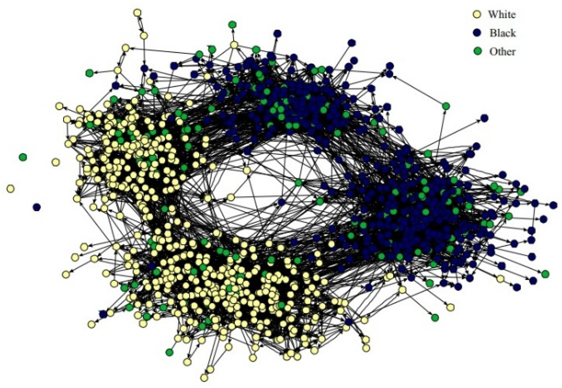
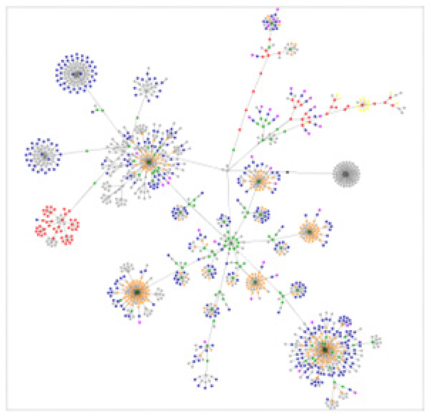
2.1. Basic Theory of Complex Networks

In the real world, there are many systems that can be expressed and analyzed by complex networks, such as common Internet, social network, aviation network, traffic network and so on. Power network is the most common complex network, and a typical complex network is shown in Figure 1.
Qian Xuesen gives a strict definition of complex networks: networks with self-organization, self-similarity, attractor, small world, part or all of the properties in scale-free [14,15]. In short, the correlation of internal factors and the characteristics of the network itself show highly complex characteristics.
Complex networks have the following main features:
(1)
Small world characteristics
The theory of Six Degrees of Separation, in the 1960s, was put forward by Stanley Milgram in his social experiment. The basic idea is that the social network can establish a contact relationship through up to 6 people.
Define an undirected network of n nodes, defined as the average minimum spacing of nodes, with
l ¯ = 1 1 2 n ( n + 1 ) i j d i j
The distance between two points is d i j , if not reached will be + , the value can be solved by combustion algorithm, which can be expressed in the mathematical field as, that if the number of nodes with a distance less than r from the center point increases with exponential r, and l will be increased by log ( n ) .
(2)
Scale-free characteristics
The number of edges of a node is called a degree. Real networks are basically designated networks and are not randomly generated. The degree distribution of nodes conforms to the power-law distribution, that is, only a few nodes have many links, such as common changes in the distribution network [16,17]. A network that meets this feature is called a scale-free network. The scale-free characteristic reflects the serious heterogeneity of the complex network, that is, the degree of the node has a serious uneven distribution, which is closely related to the robustness of the network. That is, there are attack vulnerabilities of random failures in the scale-free network, namely the high level of nodes also gives room for further optimization of the network.
There is an important index for degree, network elasticity, which refers to the reachability of the network after removing a node, which represents the robustness of the network and can be used to analyze fault recovery in the power network.
For nodes whose degree is greater than k, the cumulative distribution function of the degree of definition is:
P k = k = k k α × k 1 α
The maximum probability function in the network is:
h k = m = 1 n ( n m ) p k m ( 1 P k ) n m = ( p k + 1 P k ) n ( 1 P k ) n
k max = k h k
(3)
Superfamily characteristics
In complex networks, nodes often present group aggregation characteristics, such as families or groups, which is a typical network cohesion tendency [18], reflecting the characteristic group aggregation in a complex network. The main distribution network structure of typical power grid is family characteristic.
Family detection technology developed in recent years is a method used to explain this feature. Cluster analysis and other models are typical applications, while the concept of modularity proposed by Newman in recent years provides a clearer evaluation index of partition rationality. Generally speaking, the larger the module degree, the more reasonable the division. Newman proposed module degree calculation formula is:
Q = 1 2 m i j ( A i j k i k j 2 m ) δ ( C i , C j )
where m is the total degree in the network, A is the adjacency matrix of the network, and A i j is an integer and a non-variable that is used to describe whether there is a degree between two points, k i is a node degree and C i is a family label. Its essence is the familial difference between a network and a random network, and the greater the difference, the better the family division.
As the index of network division, module degree promotes the development of complex network detection technology, but it also has some disadvantages. In recent years, some experts have put forward module degree density and made corresponding corrections. The common detection methods include:
(1)
Methods based on graph segmentation, such as Kemighan-Lin algorithm [19], spectral bisection method and so on;
(2)
Based on hierarchical clustering methods, such as GN algorithms and Newman fast algorithms;
(3)
Based on modularity degree optimization methods, such as Greedy algorithm, Simulated annealing algorithm [20], Memetic algorithm, PSO algorithm [21], Evolutionary multi-objective optimization algorithm, etc.
The superfamily characteristics and module density after basic calculation and analysis are shown in Figure 2, which is similar to the current typical distribution network structure.

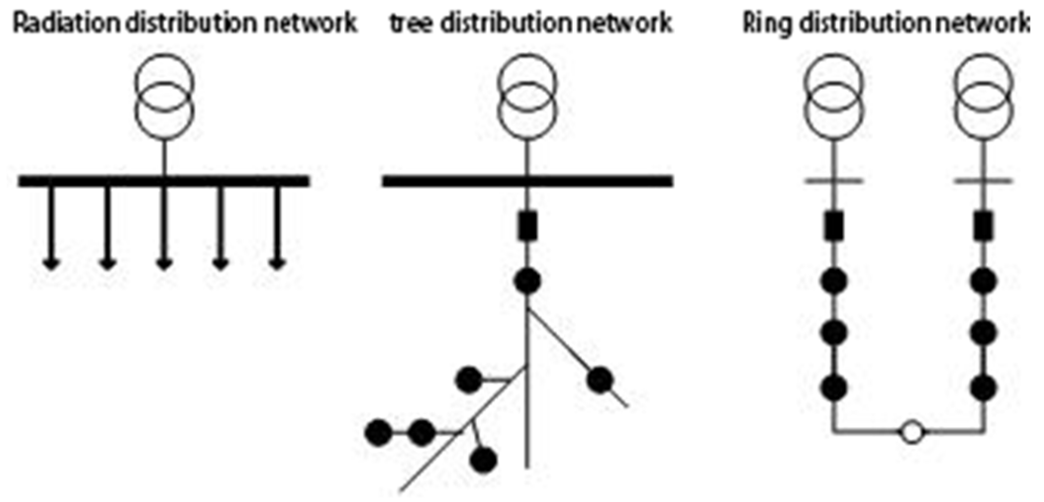
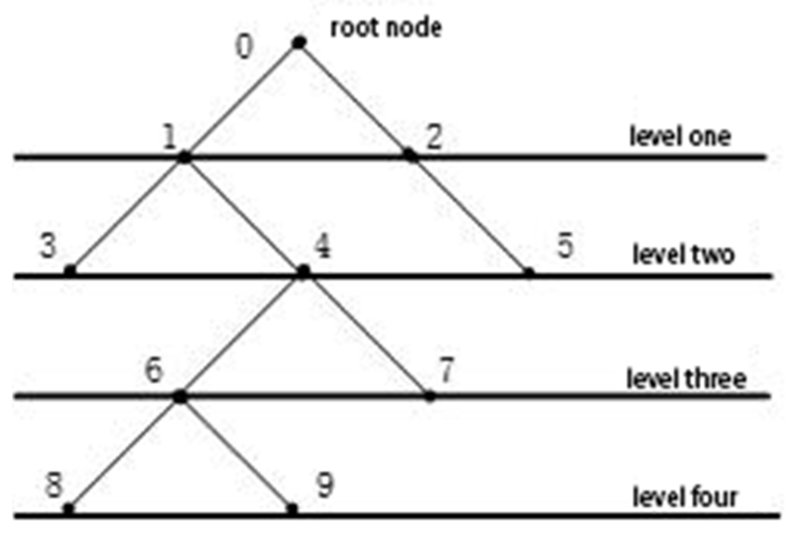
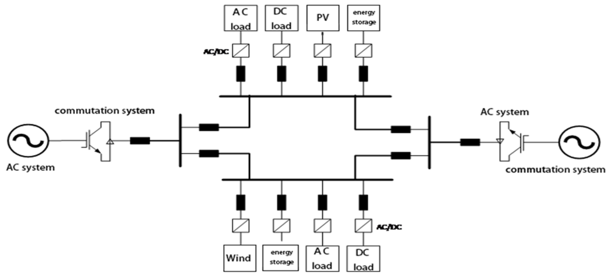
2.2. ADN Complex Network Topology

A distribution network is a network in which the secondary voltage side is directly supplied to the user after lowering the voltage in the power system [22]. It generally consists of feeder, step-down transformer, circuit breaker and various switches. Distribution network generally refers to the power grid that is 110 kV and below. In terms of topology, the distribution network can be divided into the radial network, tree network and ring network, as shown in Figure 3 below. At present, most of the distribution networks in China are tree-like structures.
Complex distribution networks can usually simplify the method and simplify the tree network diagram of one node side relationship [23]. As shown in Figure 4, make the root node as 0 and number the root node down in order according to the principle that the parent node is smaller than the child node number. The direction of the parent node to the child node is defined as the routing forward, and the branch number is the same as its child node symbol.
The topology analysis of the distribution network is the basis for other analysis of the distribution network such as state estimation, power flow calculation, fault location, isolation and power supply restoration, network reconstruction.
As the development trend of the distribution network, ADN as the main way to solve the new energy consumption, its form will be composed of multiple voltage levels of the multi-level ring network, AC-DC hybrid, interconnection interface with a unified standard, and a structure mode of flexible Ad-Hoc network based on complex network theory. Especially the DC distribution network, which is the core of the future energy internet, will become the basic supporting link, and the medium voltage distribution network that represented by flexible tributary technology will also become an important development direction in the future.
The basic topology of ADN in flexible DC mode can be divided into loop structure (Figure 5), radial structure (Figure 6) and two-terminal distribution structure (Figure 7). The analysis of ADN topology is the basis of constructing the interactive model of source, network and load under the safe operation of power grid.
Different from the traditional distribution network, there are a large number of random power supply and load nodes in the ADN network, which has a situation of bi-directional current and low-pressure transfer, and the network structure is changed into a complex undirected network structure. The physical structure of those two is consistent, so the node connection model based on graph theory has not changed fundamentally. However, the supply and demand relationship between nodes has essentially changed based on node characteristics and bi-directional current. Therefore, it is necessary to supplement node characteristics to further describe this complex undirected network. In this paper, the power flow is used as the basis of node association analysis, and the node feature vector matrix is established to analyze the complex relations between nodes.
Due to the existence of microgrid nodes in the ADN, that is, the existence of bi-directional nodes in power, which increase the complexity of network topology analysis. For the ADN, the flow direction is used as the distinction to deal with the node association. The inflow feeder node is defined as positive, and the outflow is negative. According to the characteristics of the running time, it is called as a positive node or a negative node, the power flow balance of the system can be briefly expressed as:
i = 1 N P i = 0
Which means the sum of node power is zero.
In the example of the distribution network operation mode shown in Figure 8—drawn with Microsoft Visio tools, which is different from the standard grid icon, for example—only after a simple topology sequence label is conducted for the equipment can it be found that there is a massive difference between the operation mode of the traditional unidirectional power flow system and the new bi-directional current system.
There are three main differences in the operation mode of the ADN network and the traditional distribution network:
(1)
Distributed power supply is the main difference between them;
(2)
Loop distribution network structure that is composed of a contact switch (⑧, ⑨);
(3)
Load area low-voltage transfer operation mode, which is the bi-directional current operation mode.
The so-called bi-directional current as a whole refers to the interaction way between each terminal node and the power grid, which can show two directions as a whole: inflow and outflow. However, the physical characteristics determine that the direction of power flow in a certain section of the fixed line at any time is unique, and the overall direction is from the power source to the load.
The traditional distribution network is designed according to the separation of power supply and load in the design plan. That means the power supply is sent from the fixed power network to the load center, which is in the area where the distribution busbar I is on the left side of Figure 8. The power flow output of photovoltaic and energy storage can only be within the busbar I area, and it needs to be calculated in conjunction with the main network power supply. If in the case of power failure of the main network without contact switches (⑧, ⑨), the power supply cannot be completed by the low-voltage reverse operation though the right distribution busbar II.
If bi-directional current is adopted in the right area, there is a massive difference in the operation and supply mode of each node in the distribution network. It is necessary to determine the output power and load power of each power supply according to the unidirectional power flow distribution in different feeder lines according to the network topology link relationship. Therefore, its complexity is higher than the traditional distribution network.
It can be seen that in the traditional distribution network of unidirectional power flow, it can only adopt a single feeder supply mode, and the node operation strategy is single, which indirectly leads to the waste of power generation resources. At the same time, there will be more family characteristics of human interference in this network.That is, positive and negative node planning and design on the same feeder side, which lack flexibility. At present, many hydropower enrichment areas in China, such as Sichuan, show obvious characteristics of this kind, all small hydropower according to its geographical location from 10 kV or 35 kV of unified gateway access to the power grid, to participate in the power supply.
According to the principle of maximum generation capacity (different resources required for different types of new energy), the grid connection point can be selected (when the capacity channel is sufficient) in the ADN with DER that adopts bi-directional current supply. The family characteristics in this network tend to gather around the supply-demand relationship and meet the demand of local absorption of new energy. At the same time, the network presents the characteristics of distribution network stratification. That is, the external supply-demand characteristics after family aggregation, are basically around feeder or public transformer as focal point.
The calculation flow chart is as follows Figure 9.

3. Modeling the Tightness of Node Correlation in ADN

3.1. Basic Theory of Node Tightness Analysis

Node correlation tightness is mainly used to describe the supply and demand density (complex graph theory density) of the power network based on a series of static and dynamic correlation indexes between nodes in ADN, which is used to describe the optimal matching of power supply and load under ADN operation.
The basic principle of tightness is similar to the path selection between transportation nodes. For example, one point is used to pass between two points on the map. The decision factors include road nature, road condition, adoption mode, cost, profit and loss effect and so on. By generating a fixed relationship between the two points, the effective development of transportation can be effectively guided, and different results can be obtained under different objective functions.
In the power grid, multiple types of applications can be realized through the tightness of correlation between nodes, such as power grid operation mode planning, arbitrary load according to the tightness index matching in the power node sequence to form a planning scheme. In the case of power network failure, backup power supply can be selected as the first choice for iterative calculation. In the process of constructing the index, the superfamily characteristics of network topology have been considered. The dynamic sensitivity has been selected as the index of operation analysis, which is based on the inherent node admittance matrix of the power network to form a number of influencing factors. Then, adopt the method of regional density to construct, so that the overall complexity and cost are better than the independent reconstruction of the distribution network.
The construction of tightness mainly starts from the following two aspects:
(1)
Sensitivity analysis indicators
Sensitivity calculation can describe the sensitivity of grid nodes based on various dependent variables and is the most intuitive index of response tightness. In order to further explain the relationship between node supply, the following sensitivity analysis models should be considered:
(1)
The voltage sensitivity is mainly a power sequence that characterizes the degree of voltage influence on load nodes from the perspective of power grid security. The random power supply will increase the voltage due to the output demand in ADN, which will cause the voltage flicker of the associated node and cause unnecessary production failures. This problem has become a major problem affecting the operation of the power grid in most small hydropower-intensive areas in China;
(2)
The power sensitivity is mainly based on the analysis of the reliability of the power grid, which characterizes the optimal power supply sequence of the load node. The load node with the highest sensitivity under power fluctuations of any power supply node has the highest possibility of relying on the power supply. Therefore, its reliability dependence is the highest because the efficiency matching between the two is the best;
(3)
The network loss sensitivity is mainly based on the analysis of the economics of the power grid, which characterizes the contribution of the power changes of each node to the network loss of the system. For the nodes with high sensitivity, the frequency fluctuation is not easy to reduce the loss of the power grid. Therefore, it is necessary to consider the stable operation of constant power as much as possible. For power supply nodes, it is necessary to consider power supply complementation or full consumption nearby to improve the economics of grid operation.
(2)
Static physical and statistical indicators
Static physical attributes are generally used to describe the inherent characteristics of nodes. In this paper, node capacity is selected to describe the inherent characteristics of supply and demand between nodes, to facilitate the analysis of the degree of adaptation of power and load, and to restrict safety indicators. Some other statistical indicators, such as failure rate, load loss rate, maximum or minimum power, and other analysis factors are too much involved. This article decomposes them into the constraints of their respective calculation models according to different solution goals, such as nodes failure rate, maximum and minimum power values, etc., without adding static statistical analysis. Here, it can be used as the extension of the node correlation tightness further analysis and calculation, and the node correlation tightness analysis model considering the full index set, such as security, stability, reliability, economy, etc.
After constructing the node attribute set, the TOPSIS model in complex graph theory has been used to solve the corresponding node importance index under the multi-attribute of nodes in the network.

3.2. Node Tightness Model Solution

The sensitivity calculation of the power network is generally used to study the differential relationship of various corresponding physical variables in the state of power network operation, and to obtain the sensitivity between dependent variables and independent variables. Thus, an analysis method is used to analyze the specific variables of power network operation. It is widely used in the power network, such as power network reliability analysis, network loss analysis, transmission capacity and so on, which can improve system security, system stability margin and economy.
The general expression for sensitivity is:
S x F = F x
The sensitivity value reflects the dependence of a particular network function on a particular variable, and the larger the value, the more sensitive it is, otherwise the slower it is. It quantifies the qualitative physical concept, and the calculation is simple, so it is more practical.
In this paper, we mainly rely on the establishment of power flow sensitivity matrix, which involves three kinds of variables:
Independent parameters α , including line admittance and other invariant parameters, expressed as X;
State variables X, including load node voltage, phase angle, generation node phase angle, etc., expressed as X;
The control variables V, active power and voltage of generating node, balance node voltage and phase angle, etc., are expressed as F.
At present, the main analysis and calculation of power flow sensitivity includes: ① Bus sensitivity, which is used to judge the sensitivity of weak bus or reactive power compensation position; ② Branch sensitivity, which is used to determine the sensitivity of a branch to the voltage stability of the system; ③ Generator sensitivity, which is used to determine the most important generator for voltage stability near the critical point. The method used in the calculation of power flow sensitivity mainly includes static sensitivity and trajectory sensitivity and the system is analyzed from two perspectives of static section and dynamic response, respectively.
A general expression for steady-state flow, according to the above-mentioned parameters are
{ F ( X , V ) = 0 Y = Y ( X , V )
Assuming that the stability point of the system is ( x 0 , v 0 ) , if the stability point after the system disturbance is ( x 0 + Δ x , v 0 + Δ v ) , according to Taylor expansion:
{ F ( x 0 + Δ x , v 0 + Δ v ) = F ( x 0 , v 0 ) + F x Δ x + F v Δ v = 0 y 0 + Δ y = Y ( x 0 , v 0 ) + Y x Δ x + Y v Δ v
Bring the above two into the solution:
{ Δ x = ( F x ) 1 F v Δ v = S x v Δ v Δ y = Y x Δ x + Y v Δ v = ( Y x S x v + Y v ) Δ v = S y v Δ v S x v = ( F x ) 1 F v S y v = ( Y x S x v + Y v )
The sensitivity matrix of X, Y change caused by V change.
(1)
Modeling of Node Associated Security Factors Considering Voltage Sensitivity
In this factor, the voltage is regarded as the main reference variable of system security, and the weak part of the voltage change of different nodes in the system is found through the sensitivity relationship between the power node and the load node as the judgment matrix. As a constraint on the security boundary in system operation, the system can be optimized. This factor belongs to static factor.
For the differential relation matrix of generator and load node with node voltage change, the reactive power balance equation of node injection is:
Q i V i j i V j ( G i j sin θ i j B i j cos θ i j ) Q i + j i V j B i j = 0
In order to simplify the equation, according to the previous basic method, the Taylor Formula will be expanded, and abandon the higher term and the relation is obtained as follows:
Δ Q i + j i B i j Δ V j = 0
Breakdown of generation and load nodes into matrix:
[ B L L B L G B G L B G G ] [ Δ V L Δ V G ] = [ Δ Q L Δ Q G ]
Q L and Q G are variation of load and power generation node. Note that this formula is consistent with the VQ iterative correction equation of the PQ decomposition method. It is assumed that Q L will remain the same if change the V G , then formula becomes Δ Q L = 0 .
B L L Δ V L + B G L Δ V G = 0 Δ V L = B L L 1 B G L Δ V G = S L G Δ V G S L G = B L L 1 B G L
S L G is the voltage sensitivity matrix between power generation and load nodes. Through this calculation, the power generation node that has the greatest impact on load node changes can be analyzed. Because of the power node voltage rise phenomenon in ADN, the load voltage qualification rate is affected, so according to the sensitivity matrix, it is possible to further determine the system safety boundary and the ranking of the influence of reactive power changes.
(2)
Modeling Node-related Supply Factors Considering Power Sensitivity
In this factor, the influence of power conduction change is taken as the reference variable of supply and demand reliability of nodes in the network, which mainly analyzes the dependence of power generation and load nodes, removes the influence of load loss rate in traditional reliability, and the sensitive load nodes are relatively dependent on power generation. This factor belongs to static factor.
In general, the power transfer factor of generating nodes is defined as branch power flow sensitivity, and there are:
Δ P k i = G k i Δ P i
where G k i is the generator power transfer factor, i represent generator, k represent branch. Assuming that the power transfer is completely absorbed by the balance node, the other nodes do not change, then there is:
Δ θ = X [ 0 Δ P i 0 ] T = X i Δ P
where X i is a column vector of the node impedance array, the active power flow of the branch between the node m and n changes to:
{ Δ P k i = M k T Δ θ x k = M k T X i Δ P i x k = X m i X n i x k Δ P i Δ P k i = G k i Δ P i G k i = X m i X n i x k
where M k T is the associated column vector of the node branch. The row corresponds to the node number, the independent value is 0, the entry node is −1, and the departure is 1. G k i is the transfer distribution factor, that is, generation power sensitivity. X m i represents m row i column elements in the X . If the above expression selects only nodes m it is a single node sensitivity. It can be deduced for the linkage of multiple generators:
Δ P k = G k G R Δ P G ( 0 ) G k G = [ X m i X n i x k X m j X n j x k X m l X n l x k ] G k G R = G k G F u
According to this, the adjustment amount of each generator under the active power flow change of the branch is:
Δ P G ( 0 ) = ( G k G R ) T [ G k G R ( G k G R ) T ] 1 Δ P k
According to the distributed factor formula of generation, the power transfer distribution factor between nodes can be deduced:
{ Δ P k i j = G k i j Δ P i j G k i j = X m i X m j X n i + X n j x k
(3)
Modeling of Node Correlation Economic Factors Based on Network Loss Sensitivity
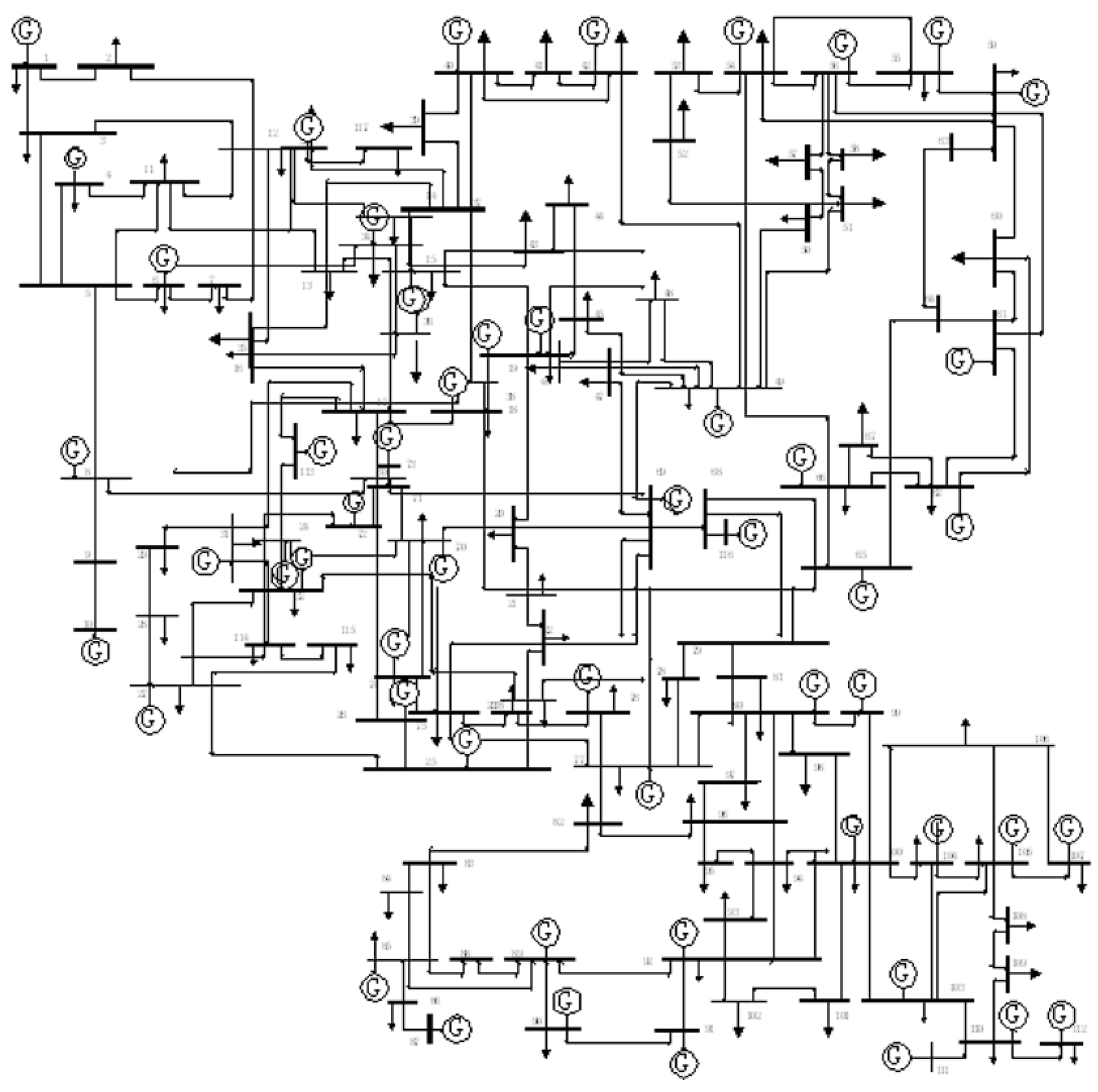
In this factor, the net loss is used to describe the economic index of the whole system. Any node voltage and branch power flow change in the ADN network will lead to the change of line loss. The network loss sensitivity as a whole reflects the system loss change caused by the node power change under the specific network operation state. The change of network loss sensitivity can guide the operation mode of the node, the load node can use as much electricity as possible at low sensitivity, and the power node can generate more electricity at high sensitivity. Unlike the first two factors, they belong to dynamic factors.
For any time t of power grid, the loss of active power network is:
P l o s s = i = 1 N j i [ α i j ( P i P j + Q i Q j ) + β i j ( Q i P j P i Q j ) ] α i j = R i j U i U j cos ( θ i θ j ) β i j = R i j U i U j sin ( θ i θ j )
where U i θ i is the voltage amplitude, Z i j = R i j + j X i j is the element of the node impedance array, and the PQ is active and reactive power, respectively.
Active and reactive sensitivity for node i can be obtained by:
G l p = P l o s s P i = 2 j i ( α i j P j β i j Q j ) G l q = P l o s s Q i = 2 j i ( α i j Q j β i j P j )
According to the relationship PQ nodes:
{ [ P l o s s P i P l o s s Q i ] = [ P i θ i U i P i U i Q i θ i U i Q i U i ] 1 [ P l o s s θ i U P l o s s U i ] U i P l o s s U i = 2 U i j = 1 N U j G i j cos θ i j P l o s s θ i = 2 U i j = 1 N U j G i j sin θ i j
Model modification for calculating physical constraints of nodes in a system.
Considering that the main solution in the system is to ensure the supply relationship of nodes, it is necessary to consider the supply and demand relationship of nodes in any family. The supply and demand capacity ratio of the superfamily supply island is basically 1:1, but considering the relationship between the islands in the system, a certain floating ratio is used as the supporting capacity factor between the islands. The general basic floating ratio is about 5%, and the basic constraint formula is:
S D ( F i ) = n N g C n / m N l C m ( C n , C m F i )
1 η S D ( F i ) 1 + η

4. Solving Examples

4.1. The Example Adopts the System Model

To verify the correctness of the example method used in this paper, the 118-node distribution network structure of the IEEE standard has been used as the calculation and analysis model of the node correlation tightness, which accords with the basic attributes of the ADN. The Matpower based on Matlab language has been used as the basis of programming. The relevant data of the example are shown in Figure 10, and the detailed parameters of the system can be obtained from the Internet.
IEEE 118 node distribution network model is a standard ADN example commonly used in electrical engineering, which contains 118 nodes, 132 branches, 15 connection lines, 117 segmented switching and xx power supply networks, which including 54 power generation nodes, and the key parameters of the system are standard values, which can be used in many scenarios. The core parameters of the 118 node network model refer to the IEEE standard model.

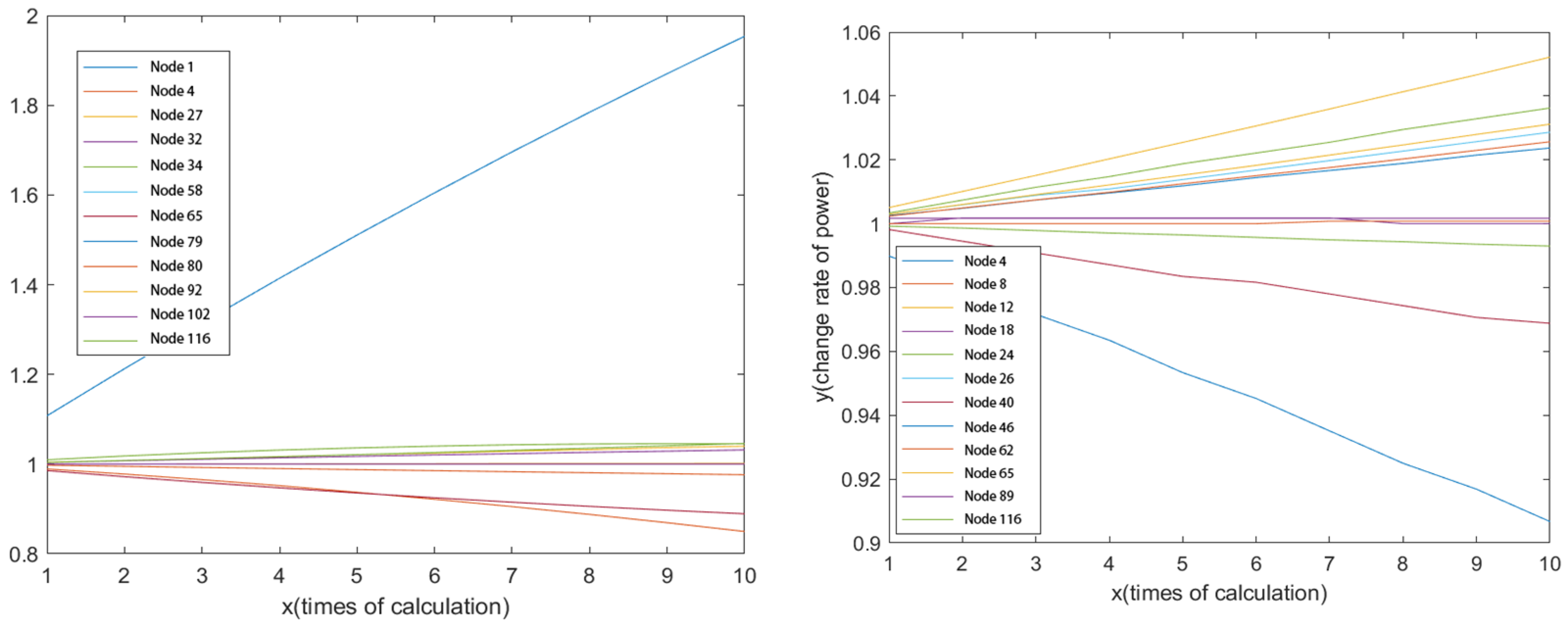
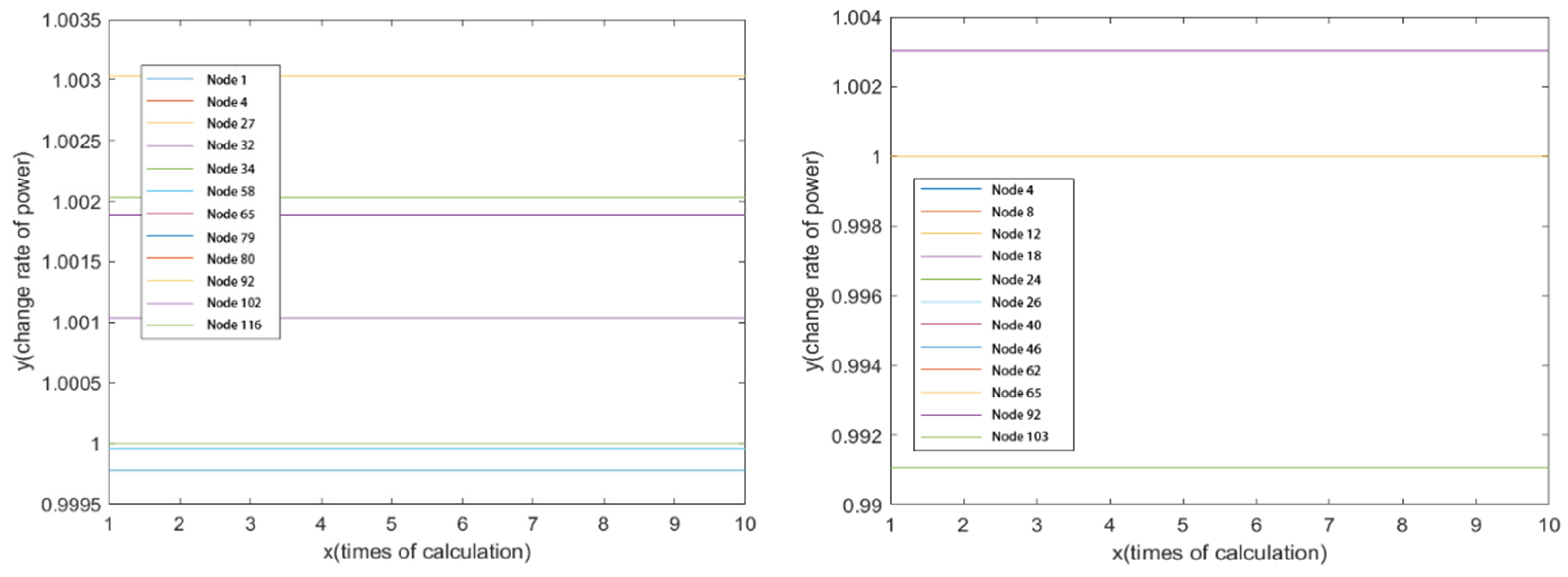
4.2. Analysis Results

The sensitivity calculation and analysis method was used to solve and analyze the 118-node distribution network. Select some of the node data, analyze and calculate the related node change rate of the whole network after the independent change of active and reactive power of the power generation node.
Select some of the power generation nodes and the change rate of the load node for example, and the result of the sensitivity change as shown in Figure 11.
The results of the node closing density matrix obtained by the whole network calculation and analysis are as follows.
In the calculation, the maximum and minimum interval limit is followed, and the theoretical basis of tightness correlation can be obtained from the diagram obviously:
(1)
In the increment node sequence, there is an obvious change rate difference. The larger the slope of the node, the more the power generation capacity is dependent on node 1;
(2)
If there is a node with a rate of change of 0, it is obviously not located in the same power supply family with node 1, which may theoretically be physically non-topological, generating node or completely independent;
(3)
There is a slope change to negative node, non-terminal node;
(4)
The change of reactive power has little effect on other nodes.
At the same time, the active power of load node is raised, the power change value of all generating nodes in the system is analyzed and observed, and the results are obtained as shown in Figure 12.
The analysis of the calculated results is basically consistent with the generation sensitivity:
(1)
Load node active power change, the most ideal state for the family generation node supply, rather than a single node;
(2)
The nodes that affect the voltage and reactive power of the load node are very few nodes, such as the No.2 load reactive power node is 92 and 103 generation nodes.
The IEEE 118 node compactness matrix is too large to be displayed in this paper, so the IEEE 14 node has been used as the basic calculation model of compactness matrix display. The compactness matrix generated by this method is as follows Figure 13.
Among them, the self-correlation coefficients are all set to 1, the matrix is a symmetric matrix, the node with a correlation value of 1 outside its own node represents the closest supply node of the node, and 0 represents the non-correlation node. The above results can be used for distribution network family analysis, distribution network topology reconstruction, scheduling optimization, and other scenarios.
Comparing the calculated matrix based on 118 nodes, it is found that the sparseness of the matrix reflects the number of distribution network supply families, that is, the number of autonomous topological islands. The sparse matrix represents a distribution network with strong autonomy, which is characterized by many distributed power sources and a complex distribution network structure. The dense matrix is basically a traditional distribution network structure, its supply relationship is radially related, and the structure is simple.
The analysis results of this matrix are most directly applied to distribution network weakness analysis and distribution network distributed power planning. By adding key associated nodes, the distribution network family and the associated characteristics are changed, and the security and flexibility of distribution network are greatly increased.

4.3. Comparative Analysis

In order to verify the correctness of the calculation method used in this paper, the standard multi-voltage level master hybrid model provided by the panda-power website is cited as the verification method, and the matlab-based matpower is used as the basis for programming implementation.
There are four voltage levels: 380 kV transmission network, 20/10 kV medium voltage distribution network, and 0.4 kV low voltage distribution network. Among them, the low-voltage distribution network presents the characteristics of high typical impedance ratio, which has the characteristics of power flow pathology, and is not easy to calculate convergence, so the forward pushback generation method is used for calculation and analysis.
In the calculation and analysis of this paper, the mature pushback generation calculation results are not analyzed, but the pypower built-in calculation model is directly used as the result, focusing on the main network using the PQ decomposition calculation results and the main network voltage and phase angle calculated by the master-slave mixed model to verify the accuracy of the model. In addition, the model here is verified by the main configuration hybrid model after stitching of the IEEE standard model, and the method is not repeated.
The initial network parameters for this model are shown in Table 1.
After 4 alternate iterations of master-slave splitting calculation, the voltage deviation of coupling node 11 gradually decreases, and the phase angle tends to be stable, meeting the convergence requirements, and the calculation is terminated. The data of iteration process is shown in Table 2.
Table 3 shows the final calculation results of each main network node calculated by PQ decomposition and the master-slave splitting method. It can be seen that its convergence and calculation results meet the requirements of calculation accuracy.

5. Conclusions

ADN was an important part of smart grid and energy internet, safe, and economic operation will be the important task, and the consumption of distributed energy was its important goal. In view of this direction, this paper proposed a distribution network node correlation tightness model based on sensitivity and physical attribute weighting, which was used to analyze the internal supply relationship between each node. The following conclusions were obtained:
(1)
Considering the main influencing factors of the relationship between nodes, using the sensitivity index as the micro-change rate determination factor, based on the three types of sensitivity of voltage, power, and network loss to reflect the three major indicators of safety, reliability, and economy;
(2)
In order to reflect the supply-demand relationship between nodes, from the three perspectives of supply capacity, responsiveness, and stability, supplementary indicators are calculated around capacity, failure rate, and flexibility margin;
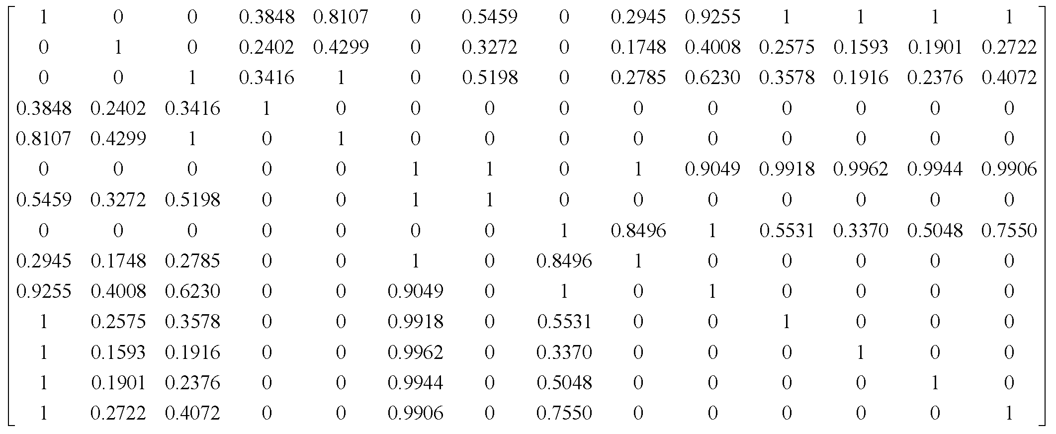
(3)
Taking into account the complexity of each index, the TOPSIS method was adopted, built around the weighted index set, calculated using AHP’s Santy scaling method, and solved using the degree concept of graph theory to form a node tightness matrix; at the same time, the ranking sequence of the most important nodes in the system can be obtained intuitively;
(4)
Compared with other related research on distribution network operation mode, the correlation tightness matrix can more flexibly present the relationship between the output indicators. Based on the weight reconstruction, a new network operation strategy can be formed quickly, and it can effectively reflect the relationship between nodes that based on the internal relationship of supply indicators, which has a wider application space.
Similarly, there were some deficiencies in this study. In the ideal active distribution network, there was no external tie line. The power supply of the high-voltage grid, which can basically meet the requirements of self-sufficiency in the network. At the same time, random power supply or load access was not considered, which had certain limitations; The limitation was that the identification of the plug and play active distribution network will have a certain delay and lag, and the identification of active distribution network planning and random access with distributed generation is low.
In the future, we will be able to more accurately analyze the dynamic correlation of each node, connect the intermittent new energy characteristics of the active distribution network in the network, and organically integrate with the relevant power prediction in the new active distribution network around the existence of plug and play, so as to make a more accurate analysis on fault recovery guidance or operation mode adjustment.

Author Contributions

Conceptualization, P.J.; Methodology, J.D.; Software, X.D.; Validation, P.J.; Formal analysis, P.J.; Investigation, H.H.; Resources, X.D. and J.D.; Data curation, P.J.; Writing—original draft, P.J., X.D., H.H. and Y.W.; Writing—review and editing, P.J.; Visualization, P.J. and Y.W.; Project administration, P.J.; Funding acquisition, P.J. All authors have read and agreed to the published version of the manuscript.

Funding

This work was funded by State Grid Economic and Technological Research Institute Co., Ltd. (Item No: SGTYHT/21-JS-223).

Informed Consent Statement

Not applicable.

Data Availability Statement

Not applicable.

Conflicts of Interest

The authors declare no conflict of interest.

References

  1. Zhao, C.; Yan, H.; Liu, D.; Zhu, H.; Wang, Y.; Chen, Y. Co-simulation research and application for Active Distribution Network based on Ptolemy II and Simulink. In Proceedings of the China International Conference on Electricity Distribution (CICED), Shenzhen, China, 23–26 September 2014; pp. 1230–1235. [Google Scholar]
  2. Zou, G.; Ma, Y.; Yang, J.; Hou, M. Multi-time scale optimal dispatch in ADN based on MILP. Int. J. Electr. Power Energy Syst. 2018, 102, 393–400. [Google Scholar] [CrossRef]
  3. Li, K.; He, Y. Evaluating nodes importance in complex network based on PageRank algorithm. AIP Conf. Proc. 2018, 1955, 040122. [Google Scholar]
  4. Fathi, R.; Tousi, B.; Galvani, S. Allocation of renewable resources with radial distribution network reconfiguration using improved salp swarm algorithm. Appl. Soft Comput. 2022, 132, 109828. [Google Scholar] [CrossRef]
  5. Anteneh, D.; Khan, B.; Mahela, O.P.; Alhelou, H.H.; Guerrero, J.M. Distribution network reliability enhancement and power loss reduction by optimal network reconfiguration. Comput. Electr. Eng. 2021, 96, 107518. [Google Scholar] [CrossRef]
  6. Li, S.; Wang, L.; Gu, X.; Zhao, H.; Sun, Y. Optimization of loop-network reconfiguration strategies to eliminate transmission line overloads in power system restoration process with wind power integration. Int. J. Electr. Power Energy Syst. 2022, 134, 107351. [Google Scholar] [CrossRef]
  7. Shahzad, K.; Amin, A.A. Optimal Planning of Distributed Energy Storage Systems in Active Distribution Networks using Advanced Heuristic Optimization Techniques. J. Electr. Eng. Technol. 2021, 16, 2447–2462. [Google Scholar] [CrossRef]
  8. Ling, P.; Fang, C.; Guo, L.; Su, X.; Zheng, S. A Novel Direct Load Flow Algorithm for Unbalanced Micro-grids Considering the Droop Characteristics of DG and Load. In Proceedings of the International Conference on Power System Technology (POWERCON), Guangzhou, China, 6–8 November 2018; pp. 2096–2101. [Google Scholar]
  9. Liao, H. Review on distribution network optimization under uncertainty. Energies 2019, 12, 3369. [Google Scholar] [CrossRef] [Green Version]
  10. Li, R.; Liu, Y.; Ouyang, G.; Long, H.; Liu, P. Research on Optimization of Planned Interruption Non-Effect for Distribution Network Planning Based on Improved Particle Swarm Optimization Algorithm. IOP Conf. Ser. Earth Environ. Sci. 2019, 252, 032071. [Google Scholar] [CrossRef]
  11. Ahmadian, A.; Elkamel, A.; Mazouz, A. An improved hybrid particle swarm optimization and tabu search algorithm for expansion planning of large dimension electric distribution network. Energies 2019, 12, 3052. [Google Scholar] [CrossRef] [Green Version]
  12. Jiang, W.; Wang, Y. Node similarity measure in directed weighted complex network based on node nearest neighbor local network relative weighted entropy. IEEE Access 2020, 8, 32432–32441. [Google Scholar] [CrossRef]
  13. Zhou, J.; Yu, X.; Lu, J.A. Node importance in controlled complex networks. IEEE Trans. Circuits Syst. II Express Briefs 2018, 66, 437–441. [Google Scholar] [CrossRef]
  14. Zhang, X.; Chen, B. Study on node importance evaluation of the high-speed passenger traffic complex network based on the Structural Hole Theory. Open Phys. 2017, 15, 1–11. [Google Scholar] [CrossRef]
  15. Amani, A.M.; Jalili, M. Power grids as complex networks: Resilience and reliability analysis. IEEE Access 2021, 9, 119010–119031. [Google Scholar] [CrossRef]
  16. Cavalcanti, T.V.; Giannitsarou, C.; Johnson, C.R. Network cohesion. Econ. Theory 2017, 64, 1–21. [Google Scholar] [CrossRef] [Green Version]
  17. Träff, J.L. Direct graph k-partitioning with a Kernighan–Lin like heuristic. Oper. Res. Lett. 2006, 34, 621–629. [Google Scholar] [CrossRef]
  18. Abou Hamad, I.; Rikvold, P.A.; Poroseva, S.V. Floridian high-voltage power-grid network partitioning and cluster optimization using simulated annealing. Phys. Procedia 2011, 15, 2–6. [Google Scholar] [CrossRef] [Green Version]
  19. Ma, K.; Yuan, C.; Xu, X.; Yang, J.; Liu, Z. Optimising regulation of aggregated thermostatically controlled loads based on multi-swarm PSO. IET Gener. Transm. Distrib. 2018, 12, 2340–2346. [Google Scholar] [CrossRef]
  20. Liu, J.; Zhou, Y.; Li, Y.; Lin, G.; Zu, W.; Cao, Y.; Qiao, X.; Sun, C.; Rehtanz, C. Modeling and Analysis Considering the Time Series Characteristics for Distribution Network with High Penetration of Renewable Energy. IET Gener. Transm. Distrib. 2020, 14, 2800–2809. [Google Scholar] [CrossRef]
  21. Aliakbary, S.; Habibi, J.; Movaghar, A. Feature Extraction from Degree Distribution for Comparison and Analysis of Complex Networks. Comput. J. 2018, 58, 2079–2091. [Google Scholar] [CrossRef] [Green Version]
  22. Choi, M.-G.; Ahn, S.-J.; Choi, J.-H.; Cho, S.-M.; Yun, S.-Y. Adaptive Protection Method of Distribution Networks using the Sensitivity Analysis for Changed Network Topologies based on Base Network Topology. IEEE Access 2020, 8, 148169–148180. [Google Scholar] [CrossRef]
  23. Levi, V.; Williamson, G.; King, J.; Terzija, V. Development of GB distribution networks with low carbon technologies and smart solutions: Scenarios and results. Int. J. Electr. Power Energy Syst. 2020, 119, 105832. [Google Scholar] [CrossRef]
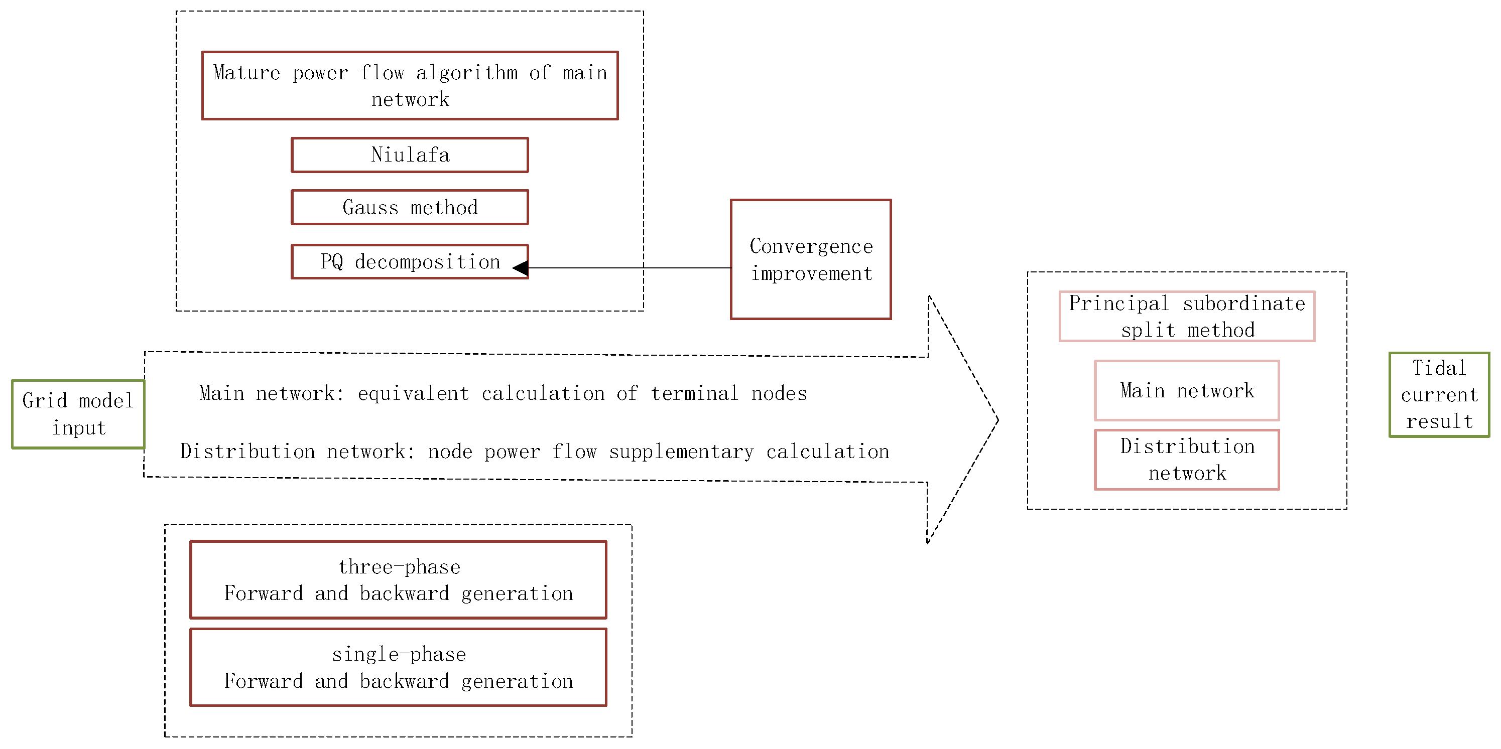
Figure 1. Complex node photo example.
Sustainability 15 00595 g001
Figure 2. Family divided of complex node example.
Sustainability 15 00595 g002
Figure 3. Typical distribution network structure.
Sustainability 15 00595 g003
Figure 4. Typical distribution network topology analysis method.
Sustainability 15 00595 g004
Figure 5. Simplify structure of loop DC distribution network.
Sustainability 15 00595 g005
Figure 6. Simplify structure of radial distribution network.
Sustainability 15 00595 g006
Figure 7. Simplified structure of Double ended DC distribution network.
Sustainability 15 00595 g007
Figure 8. Typical ADN.
Sustainability 15 00595 g008
Figure 9. Hybrid power flow algorithm flow.
Sustainability 15 00595 g009
Figure 10. Typical ADN.
Sustainability 15 00595 g010
Figure 11. Generator node sensitivity calculation result.
Sustainability 15 00595 g011
Figure 12. Load node sensitivity calculation result.
Sustainability 15 00595 g012
Figure 13. The compactness matrix generated.
Sustainability 15 00595 g013
Table 1. Initial network parameters.
Network LayeringVoltage LevelCoupling NodeNetwork SizeSolution AlgorithmConvergence Precision
Main networkAbove 10 kVNode 11Number of nodes: 20PQ decomposition1 × 10−6
Number of branches: 20
Number of power generated: 4
Distribution network0.4 kVNumber of nodes: 12Forward and backward generation
Number of branches: 11
Table 2. Calculation progress information.
RoundCoupling Node VoltageCoupling Node Phase AngleTotal Accuracy
Main NetworkDistribution NetworkDeviationMain NetworkDistribution NetworkDeviation
10.94821.00000.0517−6.8574−6.85740.00000.0517
20.94780.94820.0003−6.8842−6.85740.00000.0003
30.9478560.9478593 × 10−6−6.8844−6.85740.00003 × 10−6
40.94785630.94785632 × 10−8−6.8844−6.85740.00002 × 10−8
Table 3. Comparative analysis of results.
Network TypeNode NumberNewton’s Method Calculation ResultsThe Master-Slave Split Method Calculates the ResultDeviation
VoltagePhase AngleVoltagePhase Angle
Main network01.0301.0300
11.03257−1.737131.03257−1.737130
21.02214−3.965131.02214−3.965130
31.01445−4.628061.01445−4.628060
41.02555−3.523481.02555−3.523480
51.03−3.269181.01445−3.269180
61.00115−6.389361.02555−6.389360
71.00144−6.249991.03−6.249990
80.997036−6.319711.00115−6.319710
90.993758−6.361551.00144−6.361550
100.991537−6.369440.997036−6.369440
110.947856−6.884440.993758−6.884440
121.01237−5.793450.991537−5.793450
131.00847−5.944720.947856−5.944720
141.00443−6.113521.01237−6.113520
250.8615822.519461.008472.519460
260.8425115.750871.004435.750870
271.02616−3.523480.861582−3.523480
281.024−3.965130.842511−3.965130
291.00623−5.590551.02616−5.590550
300.990384−6.343970.990384−6.343970
Distribu-tion net-work150.990373−6.343080.990373−6.343080
160.936086−5.895450.936086−5.895450
170.92631−5.095910.92631−5.090910
180.919187−4.481880.919187−4.481880
190.914058−4.076140.914058−4.076140
200.911502−3.871550.911502−3.871550
210.923788−5.087250.923788−5.087250
220.904304−3.509680.904304−3.509680
230.8615822.519460.8615822.519460
240.8425115.750870.8425115.750870
Disclaimer/Publisher’s Note: The statements, opinions and data contained in all publications are solely those of the individual author(s) and contributor(s) and not of MDPI and/or the editor(s). MDPI and/or the editor(s) disclaim responsibility for any injury to people or property resulting from any ideas, methods, instructions or products referred to in the content.

