Influence of Traffic Parameters on the Spatial Distribution of Crashes on a Freeway to Increase Safety

Abstract

Significant research has been conducted in recent years to determine crash hotspots. This study focused on the effects of various traffic parameters, including average traffic speed and traffic volume, on the spatial distributions of freeway crashes. Specifically, this study analyzed the spatial distributions of crashes on the Qazvin–Abyek freeway in Iran using four-year crash records. Spatial crash clustering analysis was performed to identify hotspots and high cluster segments using global Moran’s I, local Moran’s I, and Getis-Ord Gi*. The global Moran’s I indicated that clusters were formed under the low range of hourly traffic volume (less than 1107 veh/h) and the high range of traffic speed (more than 97 km/h), which increased the number of heavy vehicle crashes in the early morning (time 03–06) around the 52 km segment. The results obtained from kernel density estimation (KDE), local Moran’s I, and Getis-Ord Gi* revealed similar crash hotspots. The results further showed different spatial distributions of crashes for different traffic hourly volumes, traffic speed, and crash times, and there was hotspot migration by applying different traffic conditions. These findings can be used to identify high-risk crash conditions for traffic managers and help them to make the best decisions to enhance road safety.

1. Introduction

Road crashes, which cause high rates of casualties, injuries, and financial costs, have been significant problems for the governments of developing countries, including Iran. In 2020, there were about 15,400 crash fatalities in Iran and, as reported by the Iranian Forensics Organization, around two-thirds of them occurred on suburban roads—especially on freeways.

In the last decade, many studies have been conducted on the spatial distribution of crashes (SDC) and the temporal distribution of crashes (TDC) to investigate the causes of crashes and identify crash hotspots [1,2]. Their findings prove that there is no uniform SDC and TDC (e.g., [3,4]). These results mean that there is a non-uniform distribution of crashes on different parts of roads for various reasons. Moreover, the distribution of crashes is not the same at different times, such as months of the year, days of the week, hours of the day, etc. Many studies have been conducted on the spatiotemporal distribution of crashes (STDC) [3,4,5,6,7]. For instance, Li and Zhu [2] and Plug and Xia [3] suggest an interaction between the time and location of crashes based on STDC. Moreover, the spatiotemporal analysis indicates the variations in the spatial distribution of relative crash risks at different periods, such as hours of a day, days of a week, months of a year, and different years [8,9].

Many studies explore the influence of certain parameters on road traffic safety, including behavioral factors and driver characteristics [10,11,12]. For instance, Besharati and Tavakoli Kashani [13] argue that intercity bus drivers’ behavioral characteristics significantly affect crash risks. The effects of behavioral factors and drivers’ characteristics on SDC and temporal distribution of crashes (TDC) have also been identified [14,15]. Moreover, Toran Pour and Moridpour [16] considered age and gender as parameters that affect pedestrians’ SDC and TDC. Toran Pour and Moridpour [16] also suggested different spatial distribution patterns for different human characteristics, whether for drivers or pedestrians. Anvari and Kashani [17] proved that passenger factors and the rider’s age affect rear-end motorcycle collisions, and that age and gender have a significant influence on children’s pedestrian behavior in conflict zones of urban intersections [18]. The effect of weather conditions on the SDC has also been confirmed [19].

Furthermore, several studies have focused on investigating the effects of traffic parameters such as speed and traffic volume on crash frequency and severity (e.g., [20,21,22]). According to Quddus [23], a 1% increase in average annual daily traffic (AADT) is associated with a 0.5% increase in the rates of killed and seriously injured (KSI) casualties. An increase in average traffic speed causes an increase in crash frequency. For example, a 10% increase in the average speed leads to a 30% increase in fatalities and crash severity [24].

Since the present study focuses on SDC and STDC, another attempt led to investigating the effects of traffic parameters such as hourly traffic volume and average traffic speed on SDC. Kashani and Zandi [25] found that there were entirely different TDC patterns for different hourly traffic volumes and average traffic speeds. In other words, these parameters had a significant effect on TDC. In addition, Plug and Xia [3,4] highlighted that speed is a factor that can affect TDC. Salem and Genaidy [26] also found that increasing the speed variance has an impact on SDC and increases rear-end crashes in the work zone. However, to the best of the authors’ knowledge, only a few researchers have focused on the impacts of some other traffic parameters. If the effects of traffic parameters such as average hourly traffic volume and average point speed on the SDC are proven, they can be used to identify accident hotspots in different traffic conditions. Hence, they can help traffic managers to identify conditions that pose a high crash risk. It should be noted that in the analyses, the point traffic information at the crash location is employed. However, since at the last stage of the procedure this information is related to a specific origin (and not separate road segments), it can be regarded as spatial information. This study further tried to identify the factors leading to crashes at a particular location and time. Additionally, it aimed at finding the spatiotemporal hotspots.

There are several methods for spatial analysis, including kernel density estimation (KDE), Getis-Ord Gi*, k-means clustering, and the nearest neighbor method [27]. As there was point pattern crash analysis, the KDE method was used, because it is a suitable method for identifying hotspots [27,28]. Meanwhile, KDE is the most common and well-established method and is one of the most widely used analysis methods for density estimation [1,3].

Moran’s I, Geary’s C, and Getis-Ord Gi* can be employed to find spatiotemporal autocorrelation by providing a single value of spatial autocorrelation, but they do not present the locations of clusters [16,29,30]. Despite suggesting the Bayesian approach for the spatiotemporal patterns of relative crash risks [2], several studies (e.g., Plug et al., 2011 [3]; Vemulapalli et al., 2016 [27]) have employed the co-map method for spatiotemporal analysis, and the present study was no exception. Co-map is an extension of co-plot that is a visualization tool [4]. Co-plot uses point plots and a spatial distribution pattern map, such as the KDE, to reveal the effect(s) of changing two variables [28]. Co-map can be used to investigate the temporal and spatial patterns of an event, including crime, vehicle crashes, and disease. Soltani and Askari [31] highlighted that the basis of the spatiotemporal analysis is dividing the overall parameter into subsets, and these subsets are then plotted to examine the differences among each subset. The significant relationship between SDC patterns and different conditions could help network administrators to identify specific situations to adopt proper decisions to reduce the risks of crashes.

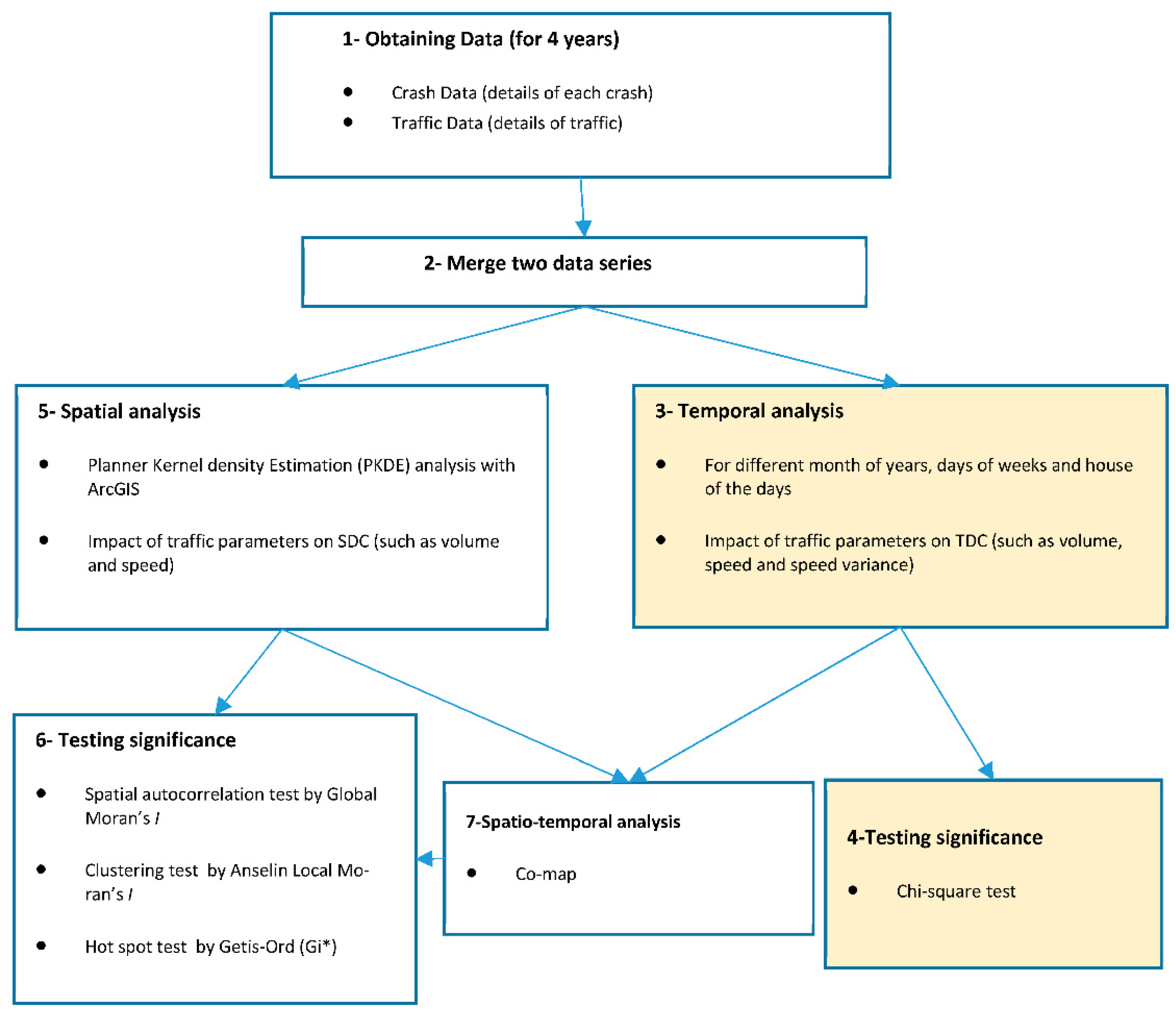
2. Methodology

The methodology of the present study is shown as a flowchart in Figure 1. It is worth mentioning that steps 3 and 4 have been previously performed by the authors and can also be followed in the work of Kashani and Zandi [25]; the rest of the steps are reported in this study. The other steps shown in Figure 1 were the main focus of this research, as follows: Step 1 is obtaining the crash and traffic datasets, and step 2 is the merging of these two data series. More explanations of steps 1 and 2 can be found in Section 3 (Case Study and Data). Step 5 is about spatial analysis, while step 6 is about testing significance and its methods; both steps are described in Section 2.1 (Spatial Analysis) and Section 2.2 (High-Frequency Crash Location). Step 7 investigates the spatiotemporal analysis, which explains the correlation of time and location of the crashes, as described in Section 1 (Introduction). In the rest of this section, the different parts of the methodology are explained.

2.1. Spatial Analysis

For spatial analysis, since KDE analysis has been used in many previous analyses, it was also employed in this research. KDE is a distance-based method generating a smooth and continuous surface map of the risk target [32]. KDE calculates a density surface within a circular distance centered at each point across a study area for identifying hazardous road situations and hotspot point events. The idea is that a crash may occurs not only at a point but with a pattern around that point, [27,29,33,34]. “Crashes on a plane within the kernels are weighted based on their Euclidean distance from the kernel center, and the resulting density value is assigned to that center. The distance is weighted according to a kernel function” [29].

For spatial analysis, both kinds of KDE—i.e., planar (2D) kernel density estimation (PKDE) and network kernel density estimation (NKDE)—are useful. PKDE reveals the density on the surface; on the other hand, NKDE shows the density along a network [35]. “NKDE is an extension of PKDE that calculates the density of point type events on a linear unit (in a network) rather than on a 2-D homogeneous area unit, as was the case of PKDE” [34].

PKDE was analyzed using ESRI ArcMap 10.4.1 software, while NKDE was estimated using SANET software [36]. Since both methods can help identify clusters, PKDE was employed more in the present study. PKDE analysis can be written as shown in Equation (1):

$$\lambda \left(s\right)={\displaystyle \sum }_{i=1}^n\frac{1}{\pi r^2}k(\frac{d_{is}}{r}),$$

(1)

where $\lambda \left(s\right)$ is the density in the location, $s$ and $r$ represent the radius (bandwidth) of KDE, and $k$ denotes the weight of point $i$ at the distance $d_{is}$ of location $s$ [34]. On the other hand, $k$ denotes the population value for each feature; in this research, the $k$ parameter was defined to the software as the crash number for each point of the path.

Moreover, “the network KDE is very similar to the planar KDE, except that the normalizing constant is $r$ instead of $\pi r^2$” [28].

A significant point in the KDE analysis is the consideration of the appropriate horizontal bandwidth value that can change the quality of the kernel estimate. To identify the optimal bandwidth, the distance increment tests for the global Moran’s I were run for different conditions and analyzed using ESRI ArcMap 10.4.1 software.

Another objective of the present study was to examine the spatial autocorrelation of traffic crashes. Strong spatial autocorrelation indicates a spatial relationship between crashes; otherwise, the crashes will occur randomly, and there is no relationship between them. As the global Moran’s I method has proven helpful for estimating the spatial autocorrelation of crashes [29,31], it was employed in this study. The global Moran’s I for autocorrelation can be written as shown in Equation (2):

$$I=\frac{n}{S_0}\frac{ {\sum }_{i=1}^n{\sum }_{j=1}^n{w}_{i,j}{z}_i{z}_j}{{\sum }_{i=1}^n{z}_i^2},$$

(2)

where $z_i$ is the deviation of an attribute for feature $i$ from its mean ($x_i$-$\overline{X}$) (Equation (3)), $w_{i,j}$ denotes the spatial weight between features $i$ and $j$, $n$ is the total number of features, and $S_0$ is the aggregate of all spatial weights (Equation (4)):

$$z_i=\frac{I-E\left[I\right]}{\sqrt{V\left[I\right]}},$$

(3)

$$S_0={\displaystyle \sum }_{i=1}^n{\displaystyle \sum }_{j=1}^n{w}_{i,j},$$

(4)

where $E\left[I\right]$ is the expected value of Moran’s I under the null hypothesis of no spatial autocorrelation, and $V\left[I\right]$ is the variance I (Equations (5) and (6)):

$$E\left[I\right]=-1/\left(n-1\right),$$

(5)

$$V\left[I\right]=E\left[I^2\right]-E{\left[I\right]}^2 .$$

(6)

The spatial autocorrelation (global Moran’s I) was also estimated using ESRI ArcMap 10.4.1 software. This software measures the spatial autocorrelation based on both locations and value features to check whether the pattern expressed is clustered, dispersed, or random. It also calculates Moran’s I index values and p-values to evaluate the significance of that index. The $w_{i,j}$ could be the crash frequency that was defined for the software as the input field (i.e., the total number of crashes or the number of crashes in the specific condition) for each point of the path.

2.2. High-Frequency Crash Locations

The spatial autocorrelation tools can identify high-frequency crash locations. They help to simultaneously measure spatial autocorrelation based on feature locations and feature values. Given a set of features and their associated attribute values, they evaluate whether a given pattern is clustered, dispersed, or random. Strong autocorrelation occurs via the global Moran’s I when the values of geographically close cells are similar. Although the global Moran’s I is a method to define spatial autocorrelation for a whole path, it cannot determine the location of the clusters locally and only provides a quick view of the condition of the spatial dependencies.

Many analysts are interested in knowing clusters’ locations and displaying them on a map, even if there is no autocorrelation. Even if there is no global spatial autocorrelation, there may still be spatial autocorrelation on some parts of the way [37]. Various cluster mapping tools have been employed for cluster analysis. With the help of these tools, places with statistically significant hot, cold, and unpleasant spatial spots can be determined.

Various cluster mapping tools can help to determine places with statistically significant hot, cold, and unpleasant spatial spots. Local indicators of spatial association (LISA) provide a measure for each spatial unit’s association and help identify the type and location of clusters [7,38,39]. However, KDE is a tool for identifying clusters. Other methods—such as KDE+, Getis-Ord Gi*, and Anselin local Moran’s I—are also used to determine hotspots. The KDE+ method, as stated by Bíl and Andrášik [40], is based on the principles of KDE that can be employed to find significant clusters and hotspot rankings.

The Getis-Ord Gi* is a widespread and valuable method to identify the spatial clusters of high value (hotspots) and of low value (cold spots) [1]. The Getis-Ord Gi* equation can be written as shown in Equation (7) [28]:

$$G_i^{*}=\frac{{\sum }_{j=1}^n{\mathrm{w}}_{i,j}\left(D\right)X_j-\overline{X}{\sum }_{j=1}^n{\mathrm{w}}_{i,j}}{\mathrm{S}\sqrt{\frac{\left[n{\sum }_{j=1}^n{\mathrm{w}}_{i,j}^2-{\left({\sum }_{j=1}^n{\mathrm{w}}_{i,j}\right)}^2\right]}{n-1}}},$$

(7)

where Gi* is the Getis-Ord Gi* value for feature $i$, ${\mathrm{w}}_{i,j}\left(D\right)$ denotes the weight between features $i$ and $j$ (i.e., the input field of the software that could be defined as the crash frequency for the desired condition), $D$ is the distance between features $i$ and $j$, $X_j$ shows the frequency at location $j,$ n reflects the number of all features, $\overline{X}$ represents the average crash frequency, and $S$ is the standard deviation of $X_j$.

The Gi* statistic is evaluated with a z-score. A higher positive z-score shows a high value of clustering, while a smaller negative z-score indicates a low value of clustering or a cold spot.

“To investigate the spatial variation as well as the spatial associations, it is possible to calculate local versions of Moran’s I” [30]. The local Moran’s I is another method for detecting high and low clusters, as well as high and low outliers. The local Moran’s I statistics of spatial association are given in Equation (8):

$$I_i=\frac{x_i-\overline{X}}{S_i^2}{\displaystyle \sum }_{j=1 j\ne i}^n{w}_{i,j}\left(x_i-\overline{X}\right),$$

(8)

where $x_i$ is an attribute for feature $i$, $\overline{X}$ represents the mean of the corresponding attribute, $S_i$ is the standard deviation, $n$ is the total number of features, and $w_{i,j}$ denotes the spatial weight between features $i$ and $j$ (i.e., the input field of the software that could be defined as the crash frequency for the desired condition). If the value of $I$ is positive, it suggests that the feature is surrounded by the same feature; thus, the feature is a part of that cluster. At the same time, the negative value of $I$ indicates that the feature is surrounded by a feature that is not similar. This type of feature is called an outlier. The Getis-Ord Gi* and the local Moran’s I index were calculated only within the standard rating framework, where the p-value can be interpreted and analyzed.

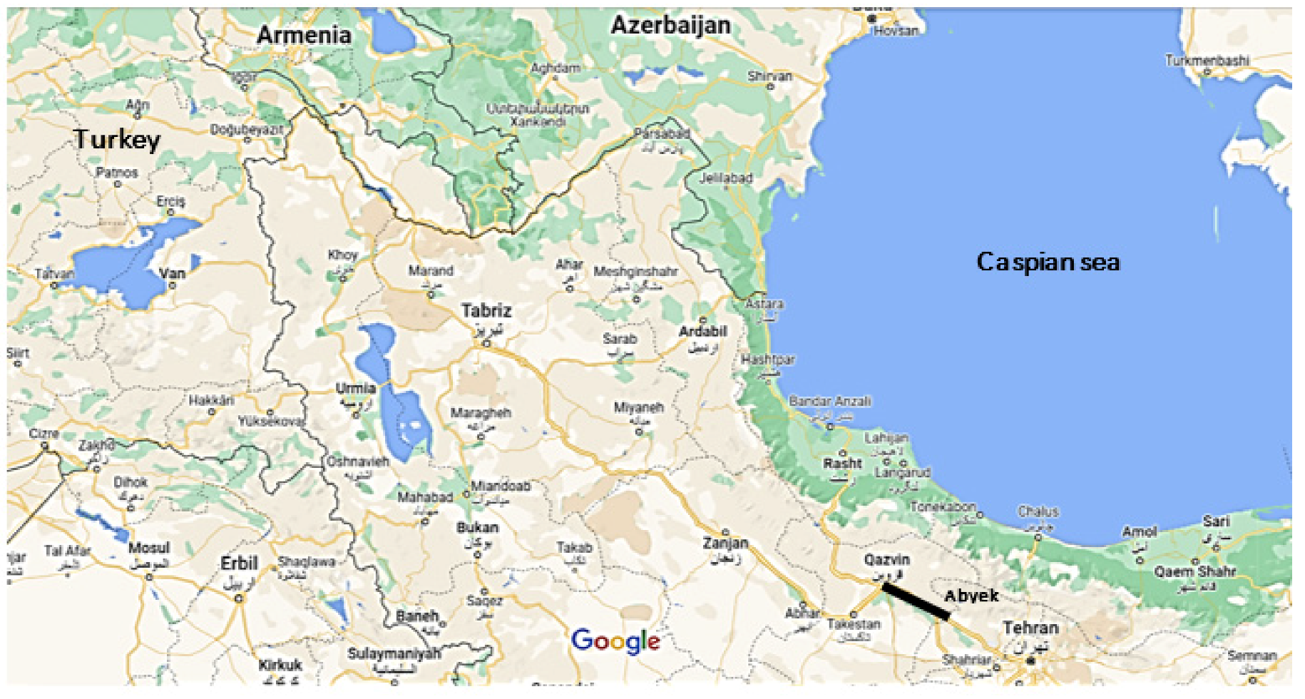
3. Case Study and Data

This research focused on a 56 km freeway between Qazvin and Abyek in Qazvin Province. This freeway connects Tehran to four provinces directly and to five other provinces indirectly. On the other hand, this freeway is also important for international transit between Iran and its northern and northwestern neighbors (Figure 2). This is a freeway in Iran with a very high crash rate (nearly 330 fatal crashes annually) and annual traffic volume (about 31 million vehicles per year). The details of the number of crashes over the past nine years are shown in

Table 1. Summary of the numbers of deaths and injuries between 2011 and 2020.

Direction	Crashes	No. of Deaths	No. of Injuries
Qazvin to Abyek	1550	204	2165
Abyek to Qazvin	1708	193	1993
Total	3258	397	4158

.

There were two datasets on this freeway’s crashes and traffic conditions. The first dataset, obtained from the traffic police of Qazvin Province, detailed the last four years‘ crash data, including the location (the crash segment), time, date, weather conditions (i.e., normal or abnormal conditions), details of the vehicles involved in the crash, drivers’ and accident victims’ characteristics (including gender and age), and types of crashes. The second dataset contained hourly traffic volumes and average traffic speeds for all types of vehicles (including cars, trucks, and trailers) on all parts of the freeway. The Iran Road Maintenance and Transportation Organization obtained these datasets via the mounted cameras and loop detectors along the route. More information about each crash was obtained by merging these two datasets. This means that some traffic data on the times and locations of crashes were further added to the crash data; thus, each record had more information about the conditions of the crashes. This study focused on crash fatalities and injuries.

4. Results and Discussion

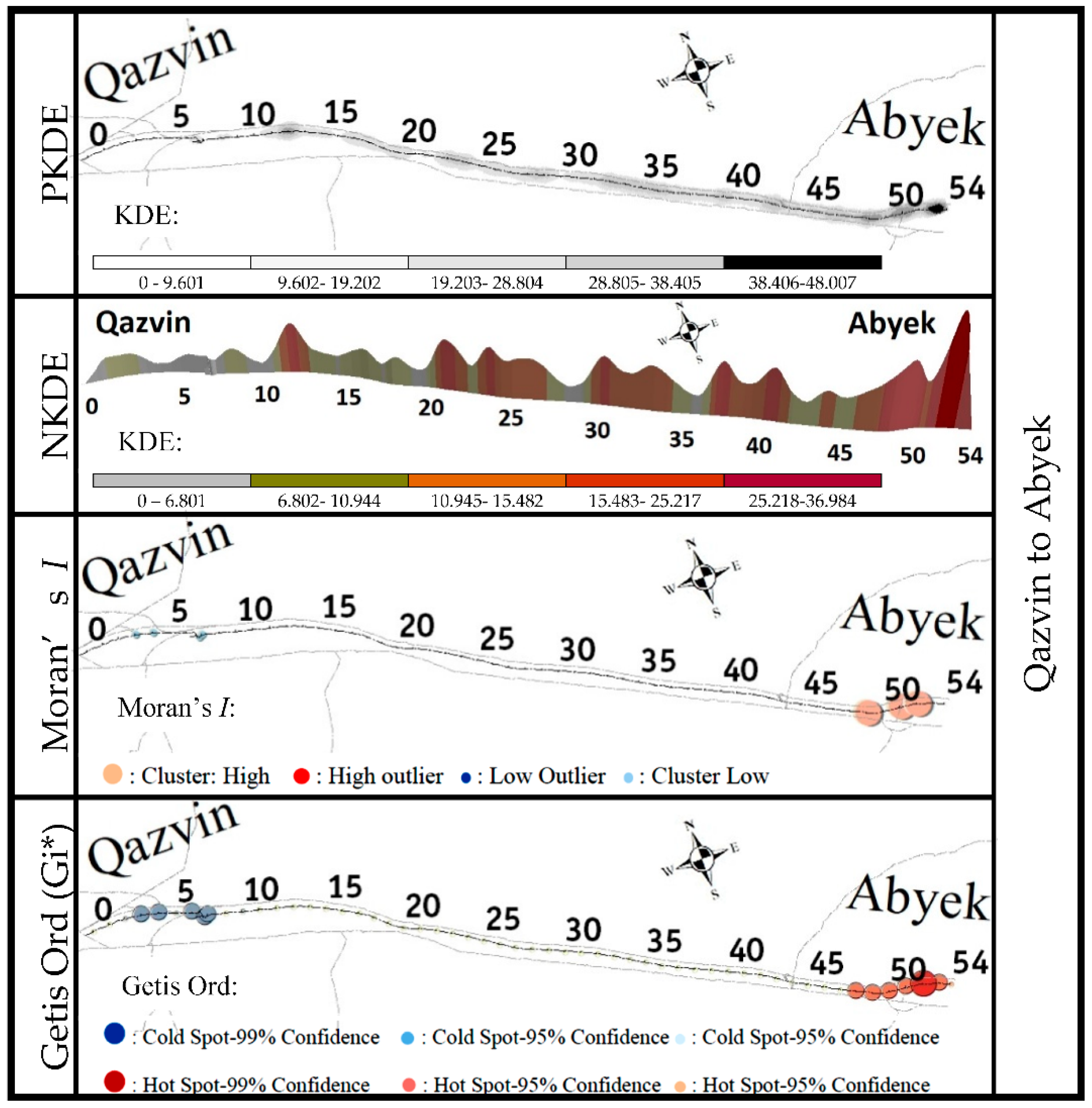
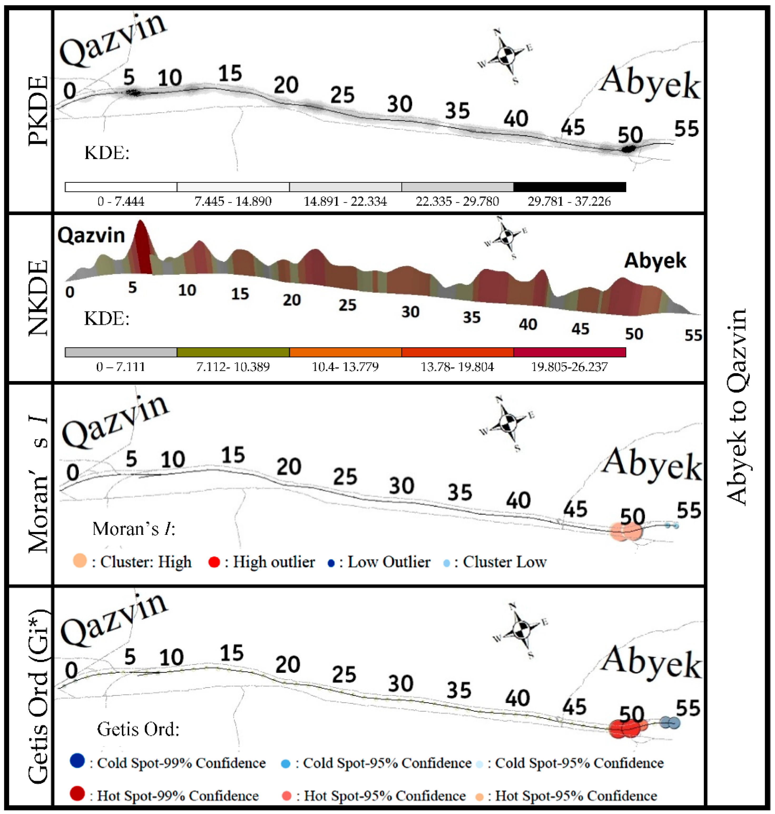
4.1. SDC Analysis

The PKDE method was run for both directions (Qazvin to Abyek and Abyek to Qazvin), and the results are shown in Figure 3 and Figure 4. The local Moran’s I and Getis-Ord Gi* methods were employed to locally identify crash clusters and hotspots. The distance increment test was run for different conditions to determine the optimal bandwidth for the global Moran’s I. Both very small and very large bandwidths could be useless. Different bandwidths are suggested for urban areas and freeways [29,41]. The results of the distance increment test can be seen in

Table 2. Incremental bandwidth test for global Moran’s I.

	Direction			Direction
	Qazvin to Abyek			Abyek to Qazvin
Distance (m)	Moran’s Index	z-Score	p-Value	Moran’s Index	z-Score	p-Value
500	0.280477	14.45204	0.00	0.262819	13.56918	0.00
600	0.253837	14.58366	0.00	0.235518	13.48739	0.00
700	0.230517	14.72402	0.00	0.204491	13.1025	0.00
800	0.194255	13.36734	0.00	0.197075	13.54769	0.00
900	0.167901	12.22441	0.00	0.168325	12.33501	0.00
1000	0.152191	11.81901	0.00	0.145903	11.38119	0.00
1100	0.163536	13.45219	0.00	0.12565	10.28813	0.00
1200	0.147651	12.63698	0.00	0.105662	9.085491	0.00

, which also contains the Moran’s I index, z-score, and p-value with 95% confidence. The results indicated that the optimal bandwidth with the highest z-score was a distance of about 700 m for Qazvin to Abyek and 800 m for Abyek to Qazvin. Since the length of the investigated crash segments was 1000 m, the 1000 m bandwidth was tested. The results indicated an acceptable p-value with 95% confidence. Thus, similar to the findings of other studies, such as the work of Mohaymany and Shahri [29], the present study’s bandwidth was set to 1000 m.

For Qazvin to Abyek, as illustrated in Figure 3, the hotspot segments identified by the Getis-Ord Gi* method with at least 95% confidence are 48, 49, 50, 51, 52, and 53, while the high clusters identified by the Moran’s I method are 49, 51, and 52. For Abyek to Qazvin, the hotspot segments obtained from the employment of the Getis Ord Gi* method with at least 95% confidence are 50, 51, and 52, whereas the high clusters determined via the Moran’s I method are 51 and 52 (Figure 4). In segment 6 of the Abyek–Qazvin freeway, some points seemed to be hotspots in PKDE, while not being high clusters or hotspots in the Getis-Ord Gi* and Moran’s I. Thus, it can be concluded that these methods did not necessarily lead to the same results.

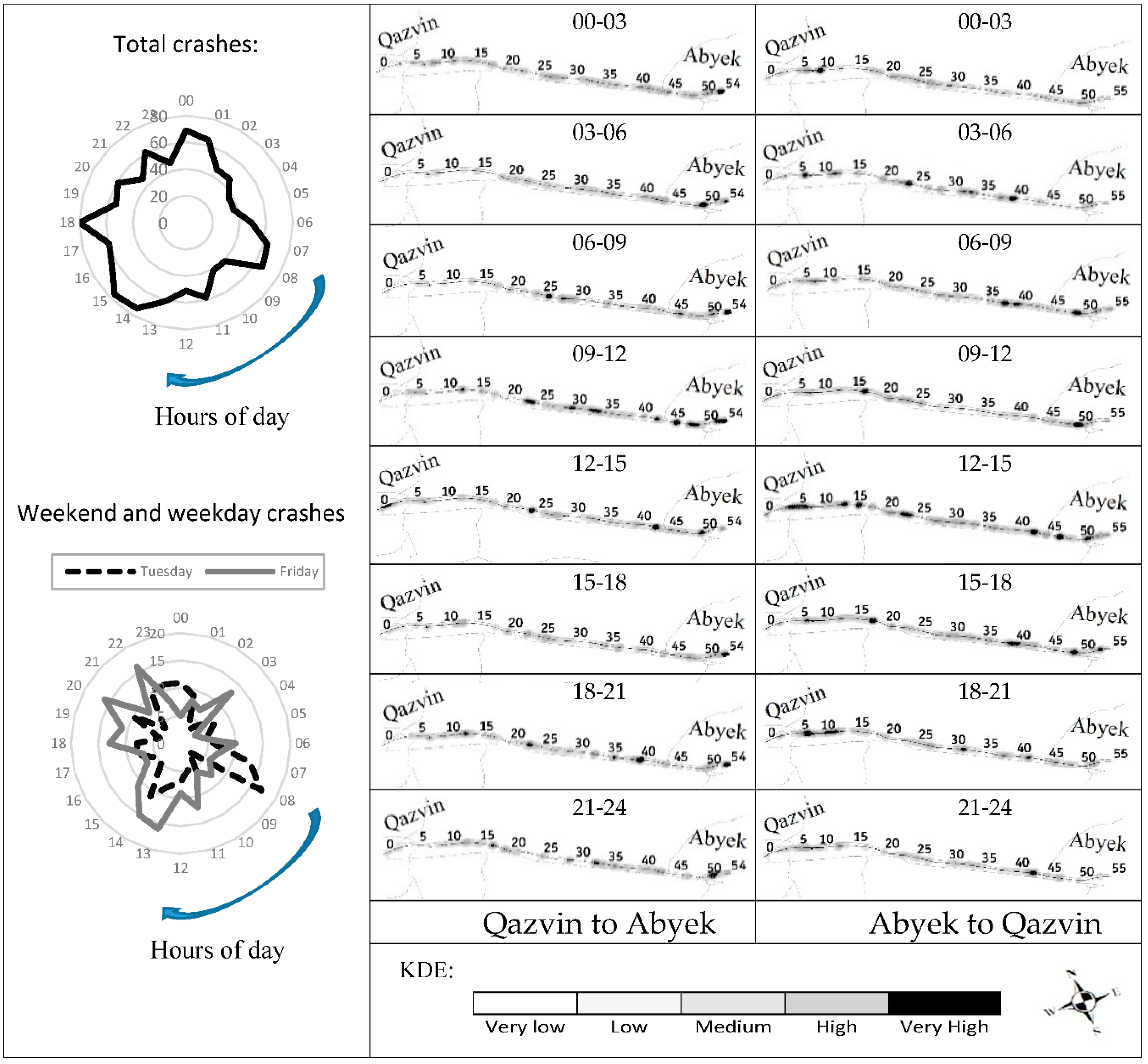
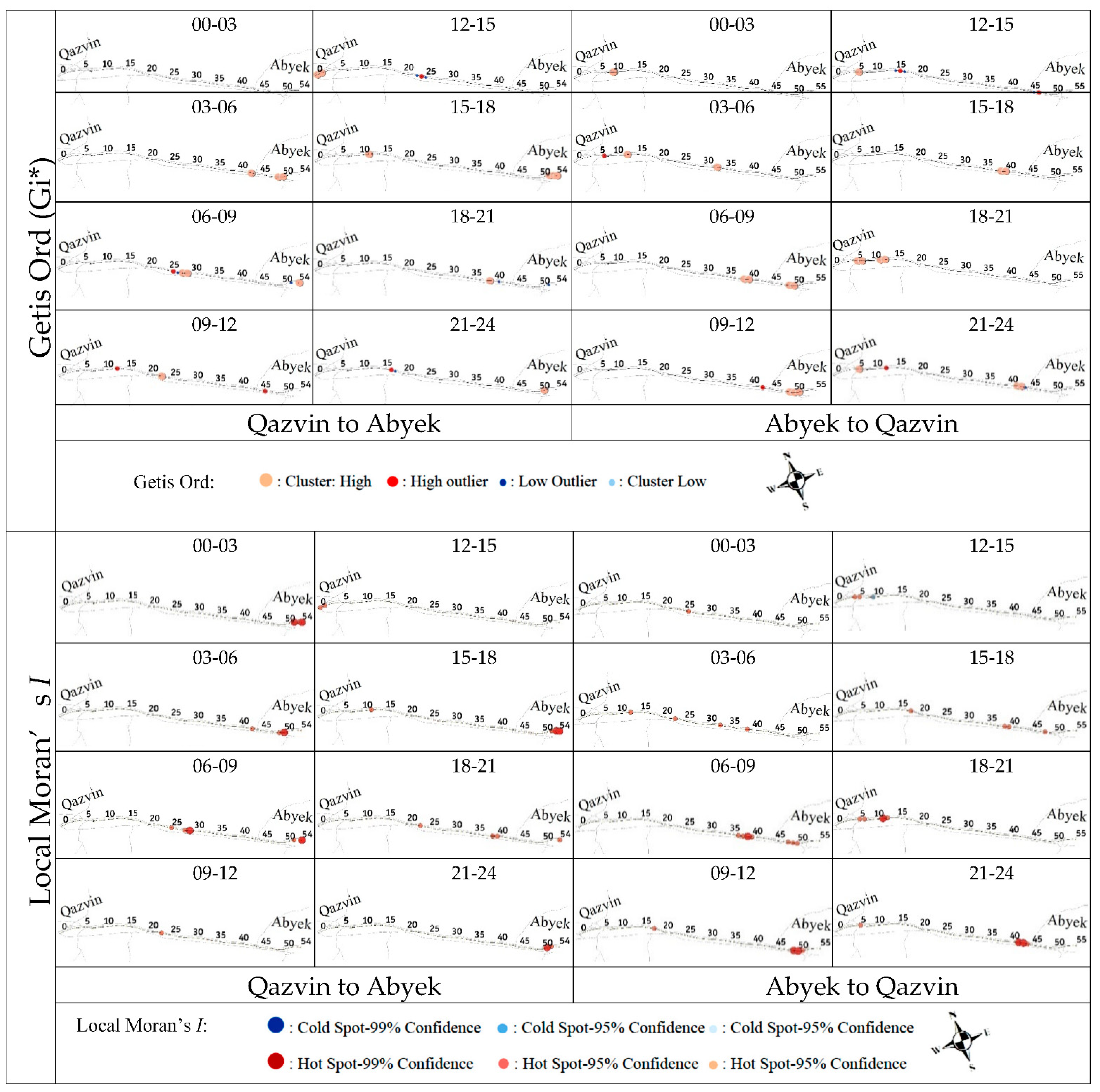
4.2. STDC Analysis

The spatiotemporal analysis of crashes was carried out by the co-map method. This method helps to compare temporal crash distribution for different conditions. The temporal part was performed with the spider plot method, consisting of two parts: one for all crashes, and the other for Friday as the weekend and Tuesday as a weekday. The data illustrated on the left side of Figure 5 indicate that the hot times for all crashes are 15, 14, and 18, while they are 08 for Tuesday and 13, 14, and 20 for Friday [25]. Of course, these times may be different for urban crashes. As an example, for urban crashes in London, the high crash times were 8:00–11:59 and 16:00–19:59 for all days of the week [42]. Figure 5 also demonstrates different TDC patterns for different conditions.

To estimate the autocorrelation between the locations and times of crashes—i.e., spatiotemporal analysis of crashes—the hours of the days were initially divided into eight equal parts. The PKDE analysis was then run for the spatial part of the analysis and for each time and direction. The right side of Figure 5 shows different hotspots for different parts of the day, i.e., morning, night, midnight, and noon. The local Moran’s I and Getis-Ord Gi* methods determined high clusters and hotspots (Figure 6). Comparing the local Moran’s I, Getis-Ord Gi*, and PKDE methods revealed many similarities. Moreover, the spatiotemporal autocorrelation analysis of the crashes showed different hotspots and high clusters for different times and locations.

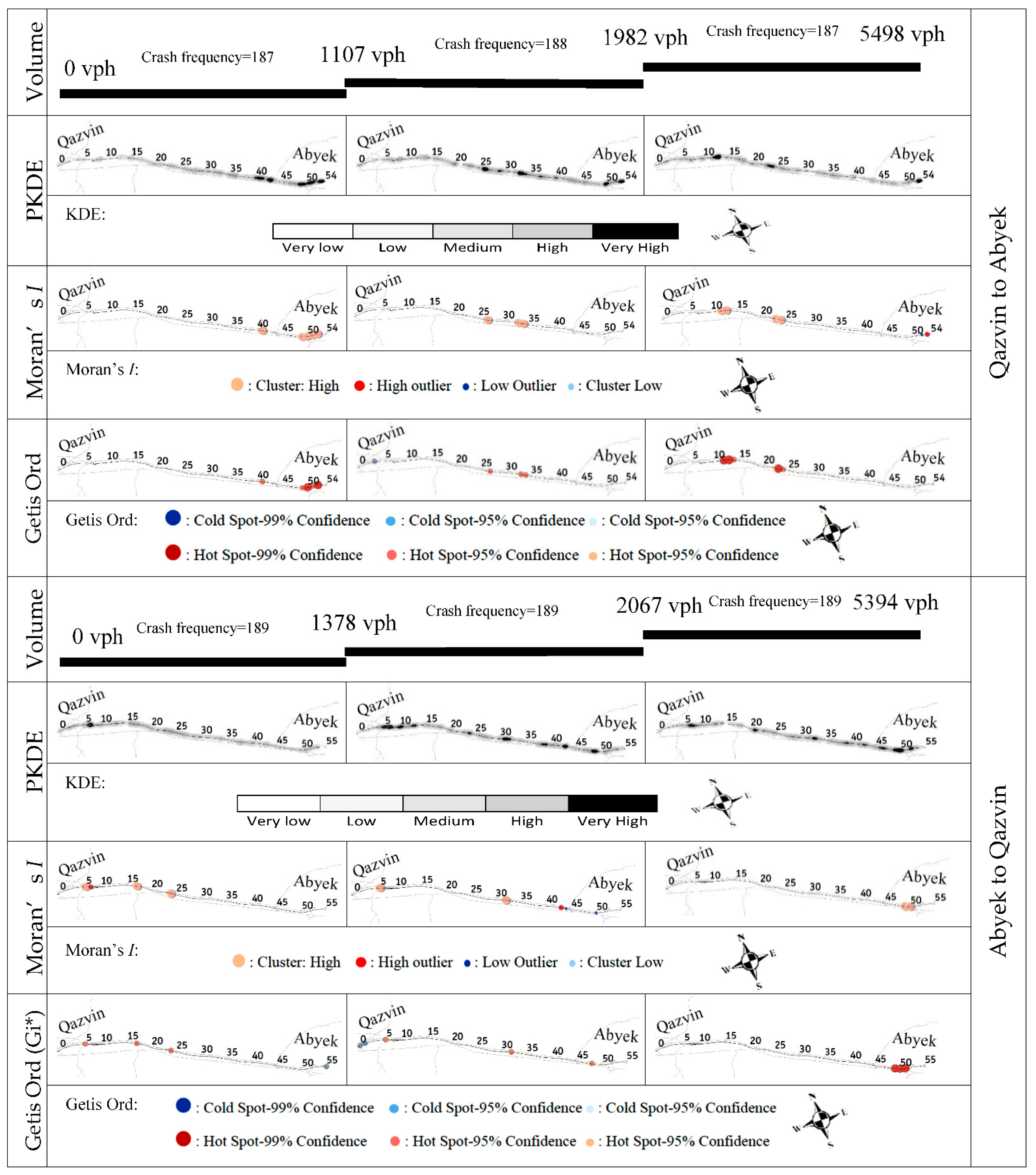
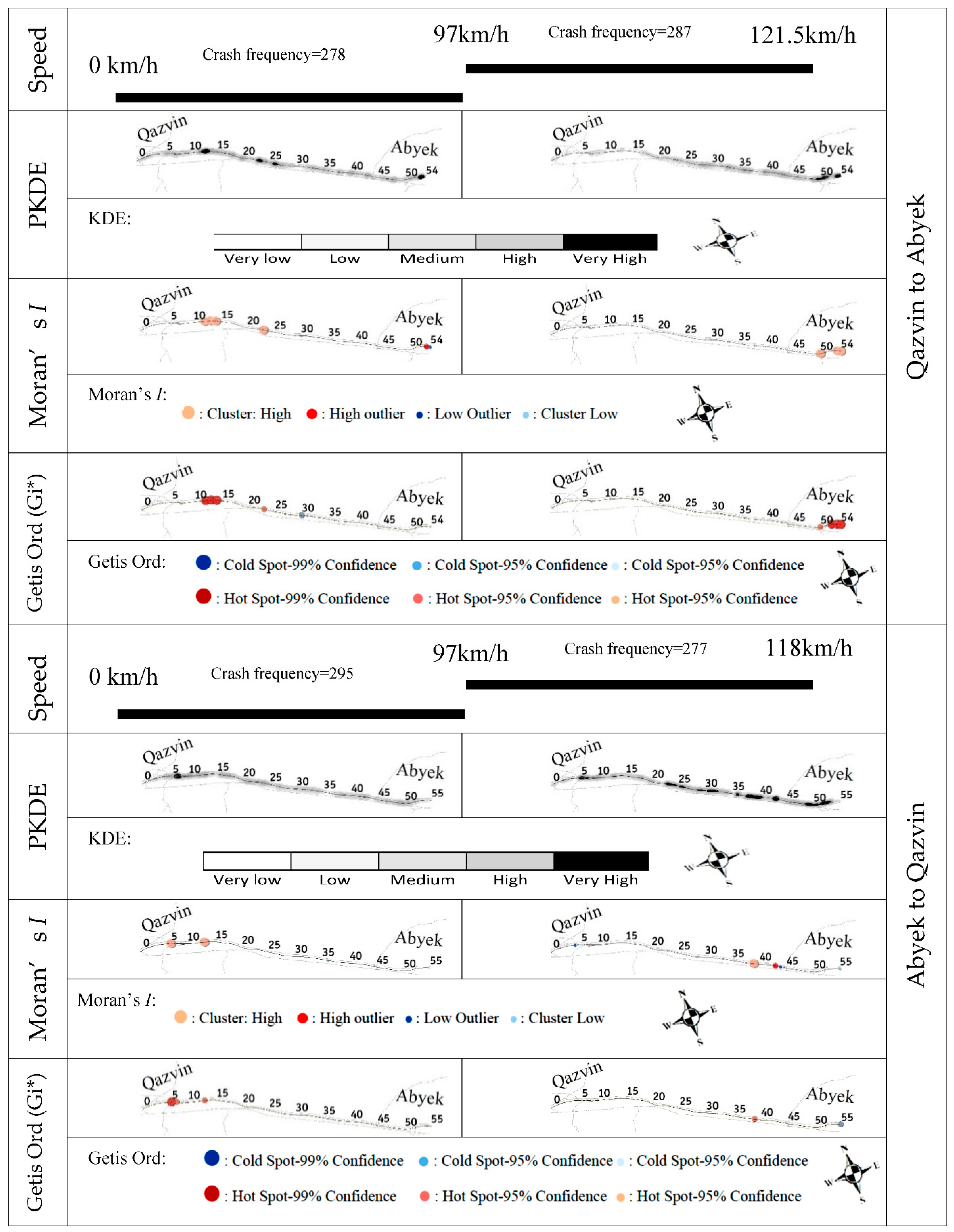
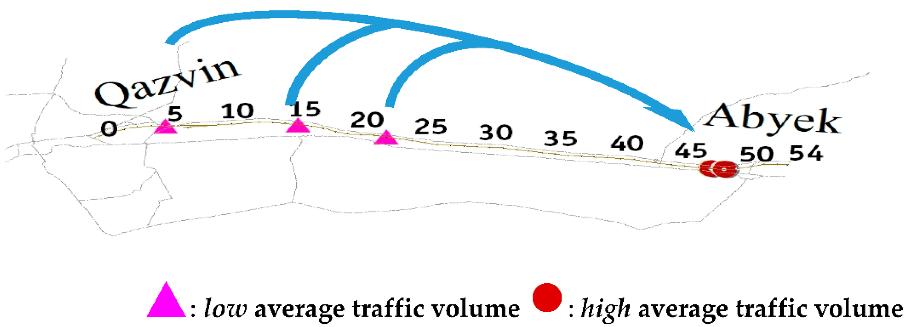
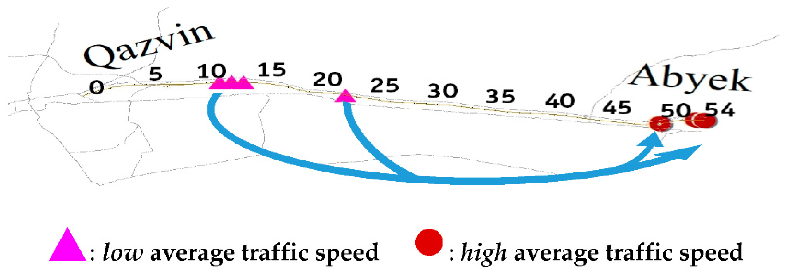
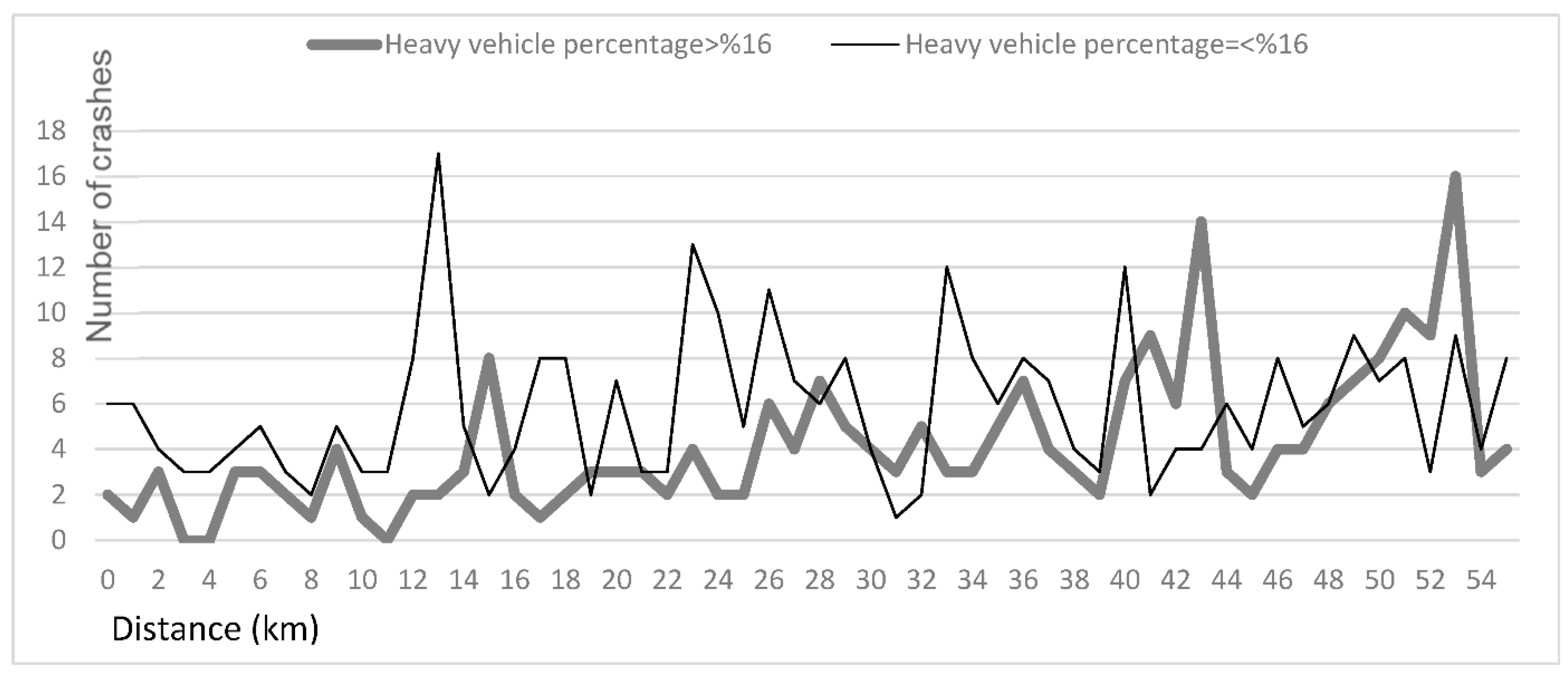
4.3. Influence of Traffic Parameters on the SDC

The main objective of this part was to investigate whether there were any significant differences between hotspots and high clusters for different hourly traffic volumes and traffic speeds. To examine the effect of hourly traffic volume on the SDC, the entire crash data were divided into three parts—low, medium, and high hourly traffic volume—so that the numbers of crashes in them were almost the same. These values and the co-map results can be seen in Figure 7, including PKDE, local Moran’s I, and Getis-Ord Gi* for both directions. The results show significant SDC differences among different volume ranges, proving the effect of hourly traffic volume on the SDC.

Similarly, the effect of average speed on the SDC was estimated. By investigating the crash frequency and mean traffic speed, it was found that the highest crash frequency occurs at nearly 95 km/h speed. In other words, the speed of 95 km/h is a marginal value at which the rates of crashes before and after it are completely different. Then, the crash data were divided into two classes: low speed, and high speed. To retain the same terms of comparison, an average speed divide point was selected to give an almost equal crash frequency (97 km/h average speed). Thus, there were two crash data classes: speeds lower and higher than 97 km/h. As illustrated in Figure 8, the results were almost identical to those of the previous step. Therefore, there were different shapes of the SDC for different traffic speeds.

For more investigating details, the impact of average hourly volume on SDC is provided in Figure 9, which focuses on the local Moran’s I hotspot migration on the Abyek–Qazvin freeway for two different conditions: low and high average traffic volume. The results show the hotspot migration from sections 5, 17, and 24 to sections 49 and 50. More information on the impact of average traffic speed on the Qazvin–Abyek freeway’s SDC is provided in Figure 10. There is hot spot migration from sections 12, 13, 14, and 23 to sections 50, 53, and 54. This proves a significant impact of both traffic volume and average speed on the SDC.

Figure 9 and Figure 10 show two examples of crash hotspot migration in different traffic conditions, which can also be extended to other conditions. Some further crash hotspot migrations can be found in Appendix A (

Table A1. Local Moran’s I output for Qazvin-to-Abyek SDC crashes.

SOURCE_ID	Accident				Low Volume				Mid Volume				High Volume				Low Speed				High Speed
	LMiIndex	LMiZScore	LMiPValue	COType	LMiIndex	LMiZScore	LMiPValue	COType	LMiIndex	LMiZScore	LMiPValue	COType	LMiIndex	LMiZScore	LMiPValue	COType	LMiIndex	LMiZScore	LMiPValue	COType	LMiIndex	LMiZScore	LMiPValue	COType
7	0.0076	2.04	0.0417	LL	0.0039	1.07	0.2848		0.0027	0.74	0.4610		0.0010	0.29	0.7746		0.0014	0.40	0.6873		0.0036	0.97	0.3324
8	0.0078	2.10	0.0353	LL	0.0042	1.15	0.2508		0.0028	0.76	0.4467		0.0010	0.29	0.7747		0.0014	0.41	0.6843		0.0033	0.89	0.3739
12	−0.0007	−0.68	0.4943		0.0005	0.49	0.6220		0.0002	0.21	0.8352		0.0063	6.52	0.0000	HH	0.0031	3.17	0.0015	HH	0.0007	0.72	0.4725
13	−0.0018	−1.29	0.1982		0.0008	0.60	0.5472		0.0001	0.07	0.9453		0.0045	3.35	0.0008	HH	0.0061	4.52	0.0000	HH	0.0016	1.14	0.2525
14	−0.0011	−1.12	0.2627		0.0003	0.35	0.7259		−0.0001	−0.11	0.9108		−0.0018	−1.83	0.0676		0.0031	3.17	0.0015	HH	0.0009	0.89	0.3761
23	0.0004	0.45	0.6499		0.0000	0.00	0.9963		−0.0005	−0.47	0.6368		0.0036	3.83	0.0001	HH	0.0019	2.02	0.0431	HH	0.0000	0.01	0.9916
24	0.0000	0.06	0.9558		0.0001	0.07	0.9451		−0.0004	−0.24	0.8072		0.0034	2.55	0.0108	HH	0.0017	1.24	0.2141		−0.0001	−0.04	0.9644
27	−0.0001	−0.08	0.9372		0.0000	0.03	0.9757		0.0020	2.05	0.0405	HH	−0.0001	−0.06	0.9527		0.0011	1.16	0.2461		0.0000	−0.03	0.9752
30	−0.0001	−0.01	0.9915		−0.0001	−0.06	0.9536		0.0000	0.01	0.9909		0.0005	0.42	0.6724		0.0026	1.97	0.0491	LL	0.0003	0.27	0.7890
33	0.0005	0.40	0.6881		−0.0003	−0.19	0.8524		0.0028	2.05	0.0406	HH	0.0001	0.12	0.9073		−0.0002	−0.11	0.9126		−0.0001	−0.06	0.9549
34	0.0013	1.01	0.3143		−0.0008	−0.57	0.5693		0.0036	2.61	0.0089	HH	−0.0002	−0.09	0.9308		−0.0001	−0.04	0.9684		0.0006	0.47	0.6407
41	−0.0002	−0.14	0.8900		0.0044	3.22	0.0013	HH	−0.0007	−0.46	0.6471		0.0003	0.26	0.7986		0.0000	0.03	0.9751		0.0008	0.60	0.5476
49	0.0027	1.99	0.0462	HH	0.0045	3.29	0.0010	HH	−0.0010	−0.69	0.4907		0.0001	0.12	0.9044		−0.0008	−0.57	0.5659		0.0020	1.48	0.1395
50	0.0019	1.94	0.0529		0.0033	3.37	0.0008	HH	−0.0014	−1.37	0.1699		0.0002	0.27	0.7849		0.0003	0.31	0.7528		0.0031	3.13	0.0017	HH
51	0.0022	2.22	0.0262	HH	0.0022	2.22	0.0264	HH	0.0001	0.11	0.9140		−0.0005	−0.54	0.5887		−0.0001	−0.08	0.9387		−0.0001	−0.09	0.9255
52	0.0050	3.67	0.0002	HH	0.0043	3.17	0.0015	HH	0.0007	0.55	0.5823		−0.0033	−2.43	0.0152	LH	0.0008	0.62	0.5325		−0.0002	−0.13	0.8938
53	0.0000	0.04	0.9702		0.0006	0.35	0.7228		−0.0014	−0.77	0.4412		−0.0051	−2.99	0.0028	HL	−0.0046	−2.67	0.0077	HL	0.0087	5.04	0.0000	HH
54	−0.0028	−1.93	0.0530		−0.0016	−1.07	0.2828		−0.0020	−1.37	0.1699		−0.0023	−1.64	0.1016		−0.0055	−3.84	0.0001	LH	0.0088	6.09	0.0000	HH

and

Table A2. Local Moran’s I output for Abyek-to-Qazvin SDC crashes.

SOURCE_ID	Accident				Low Volume				Mid Volume				High Volume				Low Speed				High Speed
	LMiIndex	LMiZScore	LMiPValue	COType	LMiIndex	LMiZScore	LMiPValue	COType	LMiIndex	LMiZScore	LMiPValue	COType	LMiIndex	LMiZScore	LMiPValue	COType	LMiIndex	LMiZScore	LMiPValue	COType	LMiIndex	LMiZScore	LMiPValue	COType
4	−0.0010	−1.03	0.3026		−0.0010	−1.04	0.2975		0.0005	0.56	0.5784		0.0001	0.13	0.8990		0.0004	0.49	0.6240		−0.0022	−2.20	0.0275	LH
5	0.0016	1.19	0.2335		0.0031	2.33	0.0196	HH	0.0045	3.25	0.0012	HH	−0.0002	−0.10	0.9205		0.0043	3.38	0.0007	HH	−0.0013	−0.89	0.3711
6	−0.0014	−0.80	0.4258		−0.0036	−2.10	0.0357	HL	0.0009	0.53	0.5927		−0.0009	−0.47	0.6380		0.0004	0.28	0.7780		−0.0009	−0.50	0.6145
13	0.0003	0.35	0.7298		0.0003	0.30	0.7656		0.0010	1.03	0.3029		−0.0005	−0.45	0.6521		0.0023	2.49	0.0126	HH	−0.0005	−0.44	0.6583
17	−0.0003	−0.16	0.8729		0.0031	2.33	0.0197	HH	0.0000	0.01	0.9918		0.0008	0.59	0.5538		0.0011	0.89	0.3743		0.0003	0.21	0.8365
24	0.0016	1.21	0.2269		0.0039	2.97	0.0030	HH	−0.0011	−0.76	0.4489		−0.0001	−0.04	0.9651		0.0002	0.19	0.8500		0.0012	0.92	0.3558
32	0.0000	0.01	0.9887		0.0003	0.34	0.7333		0.0022	2.28	0.0229	HH	−0.0001	−0.11	0.9128		0.0000	0.00	0.9988		0.0009	0.95	0.3408
36	0.0005	0.41	0.6801		0.0008	0.65	0.5131		0.0015	1.13	0.2578		−0.0004	−0.23	0.8162		0.0026	2.04	0.0412	LL	−0.0026	−1.86	0.0625
39	0.0000	−0.03	0.9762		−0.0004	−0.36	0.7179		0.0004	0.41	0.6836		0.0009	0.91	0.3603		0.0000	0.03	0.9793		0.0024	2.45	0.0142	HH
43	−0.0006	−0.42	0.6779		−0.0010	−0.71	0.4767		−0.0030	−2.12	0.0340	HL	0.0001	0.13	0.8969		−0.0004	−0.27	0.7845		−0.0040	−2.83	0.0046	HL
44	−0.0008	−0.85	0.3961		−0.0006	−0.64	0.5236		−0.0026	−2.59	0.0097	LH	−0.0007	−0.74	0.4594		−0.0007	−0.71	0.4795		−0.0020	−1.98	0.0473	LH
49	0.0008	0.61	0.5402		0.0011	0.82	0.4141		−0.0008	−0.58	0.5641		0.0060	4.38	0.0000	HH	0.0002	0.16	0.8706		0.0010	0.72	0.4721
50	0.0033	2.46	0.0140	HH	0.0000	0.06	0.9501		−0.0035	−2.49	0.0126	LH	0.0059	4.28	0.0000	HH	0.0007	0.58	0.5623		0.0016	1.14	0.2527
51	0.0048	3.55	0.0004	HH	−0.0005	−0.32	0.7502		−0.0010	−0.73	0.4660		−0.0008	−0.55	0.5827		0.0000	0.00	0.9985		0.0018	1.36	0.1738
54	0.0042	2.65	0.0081	LL	0.0027	1.72	0.0855		0.0007	0.46	0.6442		0.0024	1.50	0.1342		0.0026	1.74	0.0819		0.0018	1.13	0.2585
55	0.0041	3.17	0.0015	LL	0.0025	1.96	0.0503		0.0006	0.47	0.6406		0.0022	1.70	0.0886		0.0017	1.37	0.1707		0.0030	2.28	0.0224	LL

).

4.4. Spatial Autocorrelation between Crashes in Different Conditions

The global Moran’s I method was employed to determine the global spatial autocorrelations of crashes for both directions. As highlighted in

Table 3. The global Moran’s I for spatial crash frequency.

Direction	Moran’s I	Z	p-Value	Spatial Distribution (95% Confidence)
Qazvin to Abyek	0.436746	2.553551	0.010663	Clustered
Abyek to Qazvin	0.155543	0.991892	0.32125	Random

, there is spatial autocorrelation of crashes in the Qazvin-to-Abyek direction, with more than 95% confidence, and the crashes are clustered. However, there is a random form for the opposite direction. The global Moran’s I autocorrelation method could also be conducted for different conditions, including spatiotemporal conditions, and test the effects of some parameters—namely, hourly traffic volume and traffic speed—on the SDC. This method would show global spatial autocorrelation for different traffic volumes, speed ranges, and times of the day. According to the results provided in

Table 4. The Global Moran’s I for spatial crash frequency in different conditions.

		Condition		Moran’s I	Z	p-Value	Spatial Distribution (95% Confidence)
Direction	Qazvin to Abyek	Volume (V) (veh/h)	V < 1107	0.489669	2.846972	0.004414	Clustered
			1107 < V < 1982	0.153117	0.912806	0.361345	Random
			V > 1982	0.124857	0.823357	0.410305	Random
		Speed (S) (km/h)	S < 97	0.074382	0.527389	0.597924	Random
			S > 97	0.698778	3.989106	0.000066	Clustered
		Time (hours)	00–03	0.066896	0.492272	0.622527	Random
			03–06	0.524641	3.042979	0.002342	Clustered
			06–09	0.177791	1.094382	0.273788	Random
			09–12	0.045235	0.352046	0.724804	Random
			12–15	−0.203112	−1.036415	0.300009	Random
			15–18	0.181377	1.109924	0.267032	Random
			18–21	0.089734	0.621703	0.534137	Random
			21–24	0.003544	0.12394	0.901363	Random
	Abyek to Qazvin	Volume (V) (veh/h)	V < 1378	0.102881	0.703368	0.481827	Random
			1378 < V < 1982	0.055929	0.417969	0.67597	Random
			V > 2067	0.393178	2.33552	0.019516	Clustered
		Speed (S) (km/h)	S < 97	0.202809	1.347552	0.177802	Random
			S > 97	−0.114638	−0.5438	0.586579	Random
		Time (hours)	00–03	0.153025	0.985104	0.324573	Random
			03–06	−0.141334	−0.700012	0.48392	Random
			06–09	−0.010544	0.044112	0.964815	Random
			09–12	−0.045932	−0.159563	0.873225	Random
			12–15	−0.151469	−0.75118	0.452544	Random
			15–18	0.063173	0.464509	0.642283	Random
			18–21	0.160602	0.778682	0.436167	Random
			21–24	0.057169	0.443945	0.657082	Random

, there are spatial clusters in some conditions. For instance, in the Abyek-to-Qazvin direction, there is a spatial crash clustering only in the high range of hourly traffic volume, whereas there is a random spatial autocorrelation of crashes for other conditions.

In the Qazvin-to-Abyek direction, there is a spatial crash clustering with 95% confidence for the low range of hourly traffic volume, high range of speed, and time from 03 to 06, while for other conditions the crashes occur randomly. The location of the crash clusters for all conditions was the same and close to 52 km. To further investigate the causes of these conditions, the geometric characteristics of this path—such as curves, slopes, cross-sections, and vertical alignment—were reviewed. The results indicated that the only specific observed case in that segment was a high downhill (3%) slope.

According to Iran’s Highway Geometric Design Code, this slope, with a length of about 5.5 km, is located at the upper limit of the allowable slope. The long length and high percentage of the downhill slope are influential factors in increasing the number of heavy vehicle crashes [43]. Therefore, in the next step, the effect of the percentage of heavy vehicles on the SDC was investigated. The average percentage of heavy vehicles was 16% for the whole condition. To examine the impact of heavy vehicles, the SDC was analyzed in two modes: the lower percentage (>16%) and the higher percentage than the average of heavy vehicles (>16%). The output of the analysis is shown in Figure 11. The results showed that when the percentage of heavy vehicles was high, the highest crash frequency occurred around the 52 km segment; meanwhile, in the case of the low percentage of heavy vehicles, some other parts had a greater crash frequency. Then, the effect of the heavy vehicles in crashes (responsible and non-culpable) was analyzed (

Table 5. Crash number and percentage details for heavy vehicles.

Crash Percentage for Heavy Vehicle Non-Culpable	Crash Number for Heavy Vehicle Non-Culpable	Crash Percentage for Heavy Vehicle Responsible	Crash Number for Heavy Vehicle Responsible	Crash Frequency	Time
0.185507246	128	0.137681159	95	690	0–24
0.25	19	0.184210526	14	76	03–06

). The investigation of the effect of the percentage of heavy vehicles involved in crashes indicated that, in general, the percentage of heavy vehicles responsible for crashes was approximately 13.7%. The percentage of non-culpable heavy vehicles involved in accidents was about 18.5%. However, these values, which differed from the average values, were equal to 18.4% and 25% between 03 and 06 in the morning. Thus, the effect of the heavy vehicle percentage on the clustering of accidents in the above conditions was confirmed.

Several techniques are available to investigate the correlation between these different parameters. Among them, Pearson’s correlation test is one of the simplest and most well-known methods. Hence, this study used Pearson’s correlation test technique. It is noteworthy that the correlation coefficients near 1 denote high correlations, while those parameters with correlation coefficients near 0 are non-correlated. According to the results shown in

Table 6. Pearson’s correlation for different conditions.

	LV	HS	T0306	HVP
LV	1	0.801 **	0.568 **	0.891 **
HS	0.801 **	1	0.487 **	0.701 **
T0306	0.568 **	0.487 **	1	0.565 **
HVP	0.891 **	0.701 **	0.565 **	1

**. Correlation is significant at the 0.01 level (2-tailed). LV: low hourly traffic volume (veh/h); HS: high mean traffic speed (km/h). T0306: time 03–06; HVP: heavy vehicle percentage > 16%.

, there is very strong correlation between low traffic volume and high heavy vehicle percentage, as well as between low traffic volume and high traffic mean speed (Pearson’s correlation > 0.8). There is a strong correlation between high heavy vehicle percentage and high traffic mean speed (0.8 > Pearson’s correlation > 0.6). All correlations between parameters were significant with 95% confidence. The results indicated that these parameters had similar crash patterns for parts, i.e., the segments had almost the same crash conditions for high average traffic speed, low hourly traffic volume, and high heavy vehicle percentage. The time 03–06 had a medium correlation with the other parameters. Since this result was not just for hotspot segments but for whole parts of the road, it can be concluded that these parameters have a practical simultaneous effect on the number of crashes.

5. Conclusions

The main objective of this study was to investigate a method for a freeway in Iran to help traffic managers identify the high-risk times, locations, and conditions to make proper decisions. The primary step of this study was to conduct spatial, spatiotemporal, and density analyses of the crashes. Various methods, including PKDE, local Moran’s I, and Getis-Ord Gi*, were employed to identify the hotspots and high-crash-density segments along the route. The results revealed different hotspots and high clusters for different times. Then, the effects of some traffic parameters—namely, hourly traffic volume and speed—on the SDC were investigated globally by global Moran’s I and locally by the PKDE, local Moran’s I, and Getis-Ord Gi* methods. The findings revealed different hotspots and high clusters for different traffic conditions, and some sections were found to be more likely to experience a crash.

Moreover, according to the findings, the combination of high mean traffic speed, low traffic volume, and high downhill slope in the early morning could increase the odds of crashes, especially for heavy vehicles. These conditions caused crash clustering. These results could help traffic managers to make a suitable decision when these conditions occur. Such management could be developed into real-time traffic management systems that predict real-time crashes and estimate the crash risk using high-resolution detector data [44,45]. For these conditions, further attention is required, namely, specific speed limitations, more police control, prohibition of the entry of heavy vehicles on special days and situations, and increasing drivers’ awareness of high-risk states through VMS or other on-trip information systems. Such a real-time traffic management system could be developed in future studies.

This study focused only on fatality- and injury-related crash data because the damage-only crash data were not accessible, which was one important limitation of this research. Access to the above information could increase the accuracy of future studies.

In addition, further studies investigating the impact rates of different factors via modeling could help us to learn more about the factors affecting the clustering of crashes. Modeling based on investigating the role of geometric road characteristics could also be beneficial. Determining the extent to which these factors affect STDC could be the focus of future studies. The influence of factors other than SDC and STDC, including human characteristics and weather conditions, could be further examined. Although the present study could be extended in many ways, the analyses developed in this paper are applicable to other similar freeways and provide useful information for traffic management.

References

- Prasannakumar, V.; Vijith, H.; Charutha, R.; Geetha, N. Spatio-temporal clustering of road accidents: GIS based analysis and assessment. J. Transp. Geogr. 2011, 21, 317–325. [Google Scholar] [CrossRef]
- Li, L.; Zhu, L.; Sui, D.Z. A GIS-based Bayesian approach for analyzing spatial–temporal patterns of intra-city motor vehicle crashes. J. Transp. Geogr. 2007, 15, 274–285. [Google Scholar] [CrossRef]
- Plug, C.; Xia, J.; Caulfield, C. Spatial and temporal visualisation techniques for crash analysis. Accid. Anal. Prev. 2011, 43, 1937–1946. [Google Scholar] [CrossRef] [PubMed]
- Xia, J.C. Data mining of driver characteristics to spatial and temporal hotspots of single vehicle crashes in Western Australia. In Proceedings of 19th International Congress on Modelling and Simulation; Modelling and Simulation Society of Australia and New Zealand: Perth, Australia, 2011. [Google Scholar]
- Eckley, D.C.; Curtin, K.M. Evaluating the spatiotemporal clustering of traffic incidents. Comput. Environ. Urban Syst. 2013, 37, 70–81. [Google Scholar] [CrossRef]
- Kulldorff, M.; Hjalmars, U. The Knox Method and Other Tests for Space-Time Interaction. Biometrics 1999, 55, 544–552. [Google Scholar] [CrossRef]
- Matkan, A.A.; Mohaymany, A.S.; Shahri, M.; Mirbagheri, B. Detecting the spatial–temporal autocorrelation among crash frequencies in urban areas. Can. J. Civ. Eng. 2013, 40, 195–203. [Google Scholar] [CrossRef]
- Li, X.; Liu, J.; Zhang, Z.; Parrish, A.; Jones, S. A spatiotemporal analysis of motorcyclist injury severity: Findings from 20 years of crash data from Pennsylvania. Accid. Anal. Prev. 2021, 151, 105952. [Google Scholar] [CrossRef]
- Bíl, M.; Andrášik, R.; Sedoník, J. A detailed spatiotemporal analysis of traffic crash hotspots. Appl. Geogr. 2019, 107, 82–90. [Google Scholar] [CrossRef]
- Abdulhafedh, A. Road crash prediction models: Different statistical modeling approaches. J. Transp. Technol. 2017, 7, 190. [Google Scholar] [CrossRef]
- Zhao, X.; Xu, W.; Ma, J.; Li, H.; Chen, Y. An analysis of the relationship between driver characteristics and driving safety using structural equation models. Transp. Res. Part F Traffic Psychol. Behav. 2019, 62, 529–545. [Google Scholar] [CrossRef]
- Shirmohammadi, H.; Hadadi, F.; Saeedian, M. Clustering Analysis of Drivers Based on Behavioral Characteristics Regarding Road Safety. Int. J. Civ. Eng. 2019, 62, 529–545. [Google Scholar] [CrossRef]
- Besharati, M.M.; Kashani, A.T. Factors contributing to intercity commercial bus drivers’ crash involvement risk. Arch. Environ. Occup. Health 2018, 73, 243–250. [Google Scholar] [CrossRef] [PubMed]
- Kaygisiz, Ö.; Düzgün, Ş.; Yildiz, A.; Senbil, M. Spatio-temporal accident analysis for accident prevention in relation to behavioral factors in driving: The case of South Anatolian Motorway. Transp. Res. Part F Traffic Psychol. Behav. 2015, 33, 128–140. [Google Scholar] [CrossRef]
- Ulak, M.B.; Ozguven, E.E.; Spainhour, L. Age-Based Stratification of Drivers to Evaluate the Effects of Age on Crash Involvement. Transp. Res. Procedia 2017, 22, 551–560. [Google Scholar] [CrossRef]
- Toran Pour, A.; Moridpour, S.; Tay, R.; Rajabifard, A. Influence of pedestrian age and gender on spatial and temporal distribution of pedestrian crashes. Traffic Inj. Prev. 2018, 19, 81–87. [Google Scholar] [CrossRef]
- Anvari, M.B.; Kashani, A.T.; Rabieyan, R. Identifying the most important factors in the at-fault probability of motorcyclists by data mining, based on classification tree models. Int. J. Civ. Eng. 2017, 15, 653–662. [Google Scholar] [CrossRef]
- Deluka-Tibljaš, A.; Otković, I.I.; Campisi, T.; Šurdonja, S. Comparative analyses of parameters influencing children pedestrian behavior in conflict zones of urban intersections. Safety 2021, 7, 5. [Google Scholar] [CrossRef]
- Khan, G.; Qin, X.; Noyce, D.A. Spatial analysis of weather crash patterns. J. Transp. Eng. 2008, 134, 191–202. [Google Scholar] [CrossRef]
- Qu, X.; Kuang, Y.; Oh, E.; Jin, S. Safety evaluation for expressways: A comparative study for macroscopic and microscopic indicators. Traffic Inj. Prev. 2014, 15, 89–93. [Google Scholar] [CrossRef]
- Choi, S.; Oh, C.; Kim, M. Risk factors related to fatal truck crashes on Korean freeways. Traffic Inj. Prev. 2014, 15, 73–80. [Google Scholar] [CrossRef]
- Gargoum, S.A.; El-Basyouny, K. Exploring the association between speed and safety: A path analysis approach. Accid. Anal. Prev. 2016, 93, 32–40. [Google Scholar] [CrossRef] [PubMed]
- Quddus, M. Exploring the relationship between average speed, speed variation, and accident rates using spatial statistical models and GIS. J. Transp. Saf. Secur. 2013, 5, 27–45. [Google Scholar] [CrossRef]
- Theofilatos, A.; Yannis, G. A review of the effect of traffic and weather characteristics on road safety. Accid. Anal. Prev. 2014, 72, 244–256. [Google Scholar] [CrossRef] [PubMed]
- Kashani, A.T.; Zandi, K. Influence of Traffic Parameters on the Temporal Distribution of Crashes. KSCE J. Civ. Eng. 2020, 24, 954–961. [Google Scholar] [CrossRef]
- Salem, O.; Genaidy, A.; Wei, H.; Deshpande, N. Spatial distribution and characteristics of accident crashes at work zones of interstate freeways in Ohio. In Proceedings of the 2006 IEEE Intelligent Transportation Systems Conference, Toronto, ON, Canada, 17–20 September 2006. [Google Scholar]
- Vemulapalli, S.S.; Ulak, M.B.; Ozguven, E.E.; Sando, T.; Horner, M.W.; Abdelrazig, Y.; Moses, R. GIS-based spatial and temporal analysis of aging-Involved accidents: A case study of three counties in florida. Appl. Spat. Anal. Policy 2016, 10, 537–563. [Google Scholar] [CrossRef]
- Kuo, P.F.; Zeng, X.; Lord, D. Guidelines for choosing hot-spot analysis tools based on data characteristics, network restrictions, and time distributions. In Proceedings of the 91 Annual Meeting of the Transportation Research Board, College Station, TX, USA, 14 November 2011. [Google Scholar]
- Mohaymany, A.S.; Shahri, M.; Mirbagheri, B. GIS-based method for detecting high-crash-risk road segments using network kernel density estimation. Geo-Spat. Inf. Sci. 2013, 16, 113–119. [Google Scholar] [CrossRef]
- Erdogan, S. Explorative spatial analysis of traffic accident statistics and road mortality among the provinces of Turkey. J. Saf. Res. 2009, 40, 341–351. [Google Scholar] [CrossRef]
- Soltani, A.; Askari, S. Exploring spatial autocorrelation of traffic crashes based on severity. Injury 2017, 48, 637–647. [Google Scholar] [CrossRef]
- Hashimoto, S.; Yoshiki, S.; Saeki, R.; Mimura, Y.; Ando, R.; Nanba, S. Development and application of traffic accident density estimation models using kernel density estimation. J. Traffic Transp. Eng. 2016, 3, 262–270. [Google Scholar] [CrossRef]
- Boroujerdian, A.M.; Karimi, A.; Seyedabrishami, S. Identification of hazardous situations using Kernel density estimation method based on time to collision, case study: Left-turn on unsignalized intersection. Int. J. Transp. Eng. 2014, 1, 223–240. [Google Scholar]
- Benedek, J.; Ciobanu, S.M.; Man, T.C. Hotspots and social background of urban traffic crashes: A case study in Cluj-Napoca (Romania). Accid. Anal. Prev. 2016, 87, 117–126. [Google Scholar] [CrossRef] [PubMed]
- Okabe, A.; Sugihara, K. Spatial Analysis along Networks: Statistical and Computational Methods; John Wiley & Sons: Hoboken, NJ, USA, 2012. [Google Scholar]
- Okabe, A.; Okunuki, K.-I.; Shiode, S. The SANET toolbox: New methods for network spatial analysis. Trans. GIS 2006, 10, 535–550. [Google Scholar] [CrossRef]
- Loo, B.P.Y.; Anderson, T.K. Spatial Analysis Methods of Road Traffic Collisions; CRC Press: Boca Raton, FL, USA, 2015. [Google Scholar]
- Anselin, L. Local indicators of spatial association—LISA. Geogr. Anal. 1995, 27, 93–115. [Google Scholar] [CrossRef]
- Shariat-Mohaymany, A.; Shahri, M. Crash prediction modeling using a spatial semi-local model: A case study of Mashhad, Iran. Appl. Spat. Anal. Policy 2017, 10, 565–584. [Google Scholar] [CrossRef]
- Bíl, M.; Andrášik, R.; Svoboda, T.; Sedoník, J. The KDE+ software: A tool for effective identification and ranking of animal-vehicle collision hotspots along networks. Landsc. Ecol. 2016, 31, 231–237. [Google Scholar] [CrossRef]
- Okabe, A.; Satoh, T.; Sugihara, K. A kernel density estimation method for networks, its computational method and a GIS-based tool. Int. J. Geogr. Inf. Sci. 2009, 23, 7–32. [Google Scholar] [CrossRef]
- Siamidoudaran, M.; Iscioglu, E.; Siamidodaran, M. Traffic injury severity prediction along with identification of contributory factors using learning vector quantization: A case study of the city of London. SN Appl. Sci. 2019, 1, 1–13. [Google Scholar] [CrossRef]
- Zhao, L.; Zhang, X.; Zhang, Y.; Xu, T. Length of Slope Determination with Heavy Duty Vehicles. In CICTP 2020; ASCE Library: Reston, VA, USA, 2020; pp. 4255–4267. [Google Scholar]
- Hossain, M.; Muromachi, Y. A Bayesian network based framework for real-time crash prediction on the basic freeway segments of urban expressways. Accid. Anal. Prev. 2012, 45, 373–381. [Google Scholar] [CrossRef]
- Shi, Q.; Abdel-Aty, M. Big data applications in real-time traffic operation and safety monitoring and improvement on urban expressways. Transp. Res. Part C Emerg. Technol. 2015, 58, 380–394. [Google Scholar] [CrossRef]