Do Chinese Photovoltaic Products Have Trade Potential in RCEP Countries? A BP Neural-Network-Improved Trade Gravity Model Analysis

Abstract

China plays an important role in the global trade of photovoltaic products, and the RCEP agreement provides more opportunities and possibilities for China. This paper develops an improved trade gravity model with BP neural networks to estimate trade potentials, and the following conclusions are obtained: (1) The BP neural network is a more effective estimation method than traditional pooled regression, fixed effects, and random effects, and the combination of multiple neural networks for prediction can lead to higher robustness and accuracy. (2) The potential of China’s trade in PV products to RCEP countries is relatively mature, but the scale of trade in PV products between China and Japan and other countries may still be further expanded. (3) China’s trade potential for different regions in the RCEP agreement changed historically in different processes, with China’s trade potential for the Oceania region declining, while its trade potential for the East and Southeast Asia region increased in recent years.

1. Introduction

In the context of today’s global climate change conditions and traditional energy depletion, the development of renewable energy has become the political consensus and action goal of all countries. In recent years, the development of China’s renewable energy trade comprised world-renowned achievements; in 2015, China’s renewable energy product exports reached USD 260.22 billion, accounting for 18.4% of the world’s total renewable energy product exports. In 2016, China replaced the United States as the world’s largest producer and consumer of renewable energy, contributing 40% to the world’s renewable energy, which is more than the OECD organizations combined. Among them, China’s trade achievements in the field of photovoltaic products are particularly remarkable. In 2022, China’s “14th Five-Year Plan” for renewable energy development indicates that China’s renewable energy industry has strong advantages and international competitiveness in the field of photovoltaic products. Shuai [1] used the projection-tracing method and entropy method and observed that China’s renewable energy competitiveness is growing at a rapid rate. According to the UN Comtrade database, China’s share of world PV-related exports reached 27% in 2020, making it the world’s largest exporter of PV products. However, China still has some problems in the process of renewable energy development: For example, Xu [2] believes that China’s green bond market has a dominant position at present, but this dominant position has a functional flaw in that the market lacks diversity. However, overall, China has a more important position in the international trade of photovoltaic products. In January 2022, the Regional Comprehensive Economic Partnership Agreement (RCEP) officially came into force, and the agreement member countries comprised three countries in East Asia (China, South Korea, and Japan), two Oceania countries (New Zealand and Australia), and ten countries ASEAN, with a total of 15 countries, covering nearly half of the world’s population and nearly one-third of international trade.

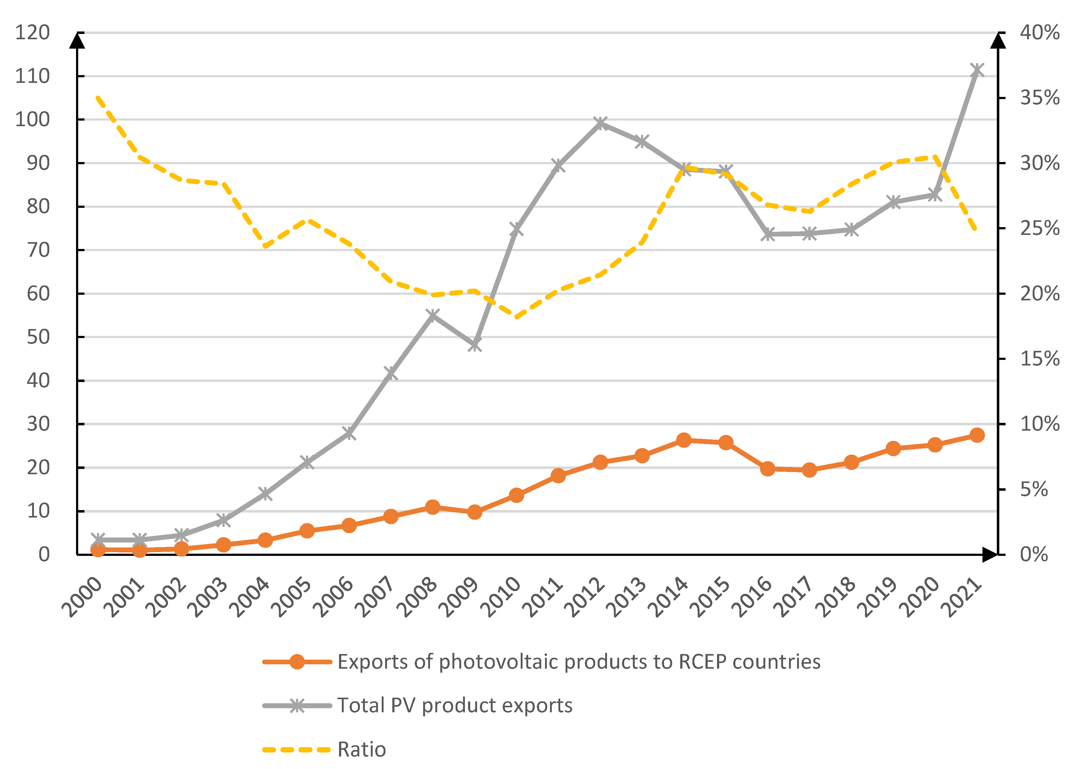
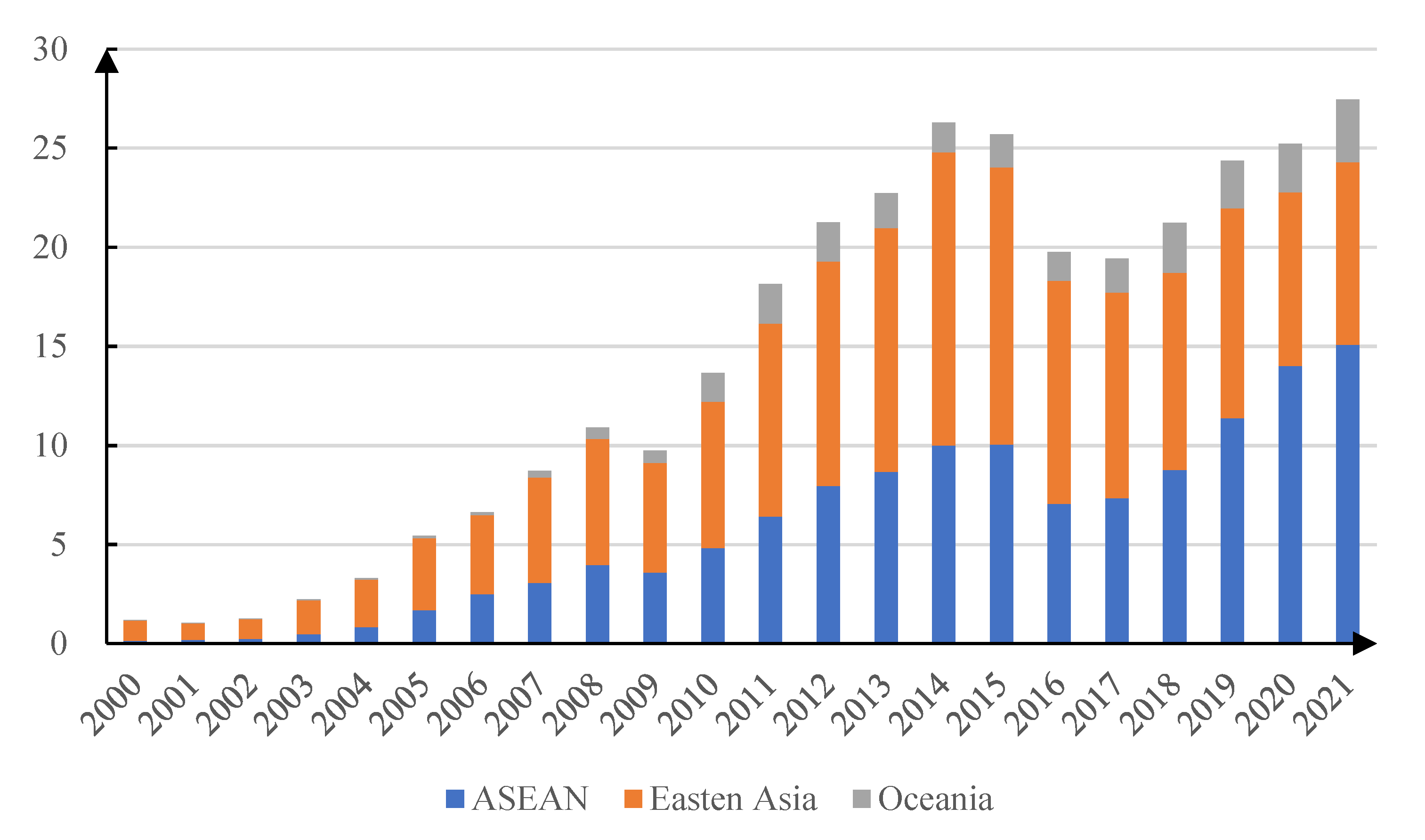
As shown in Figure 1, the region covered by the RCEP agreement was already an important market for China’s PV exports long before the agreement came into force (data from the trade database UN Comtrade). In each year between 2000 and 2021, China’s PV exports to the region accounted for more than 18% of China’s total PV exports, especially in 2000 when the ratio was as high as 33.99%. Overall, the RCEP market plays a pivotal role in the export of Chinese PV products. Moreover, as shown in Figure 2, China’s PV exports to the RCEP region also grew significantly, with the most significant growth observed in exports to ASEAN and East Asia countries. The growth of China’s PV product exports to the region is attributed to the high priority given to the construction of renewable energy facilities in the region. For example, ASEAN has set an overall regional target of 23% renewable energy shares in the primary energy mix by 2025 in the ASEAN Cooperation Action Plan 2016–2025 Phase I: 2016–2020, which provides a large market for Chinese PV products.

With the more liberal and perfect trade relations created by the agreement among its member countries, China’s PV exports can have a broader development space. However, it is also important to note that China’s trade potential with each RECP member country differs due to country-specific differences in demand, geographic distance, and other factors, and this difference will have an impact on China’s export strategy for PV products to RECP countries. Therefore, the study of China’s trade potential for renewable energy products in RCEP countries can provide a deeper understanding of China’s renewable energy export development and can provide scientific suggestions for China’s trade and cooperation with the RCEP region for PV products.

In order to address the gap in the literature on China’s trade patterns in renewable energy products for RCEP countries and the literature on the application of neural-network-improved trade gravity models on trade potential estimation, this paper constructs a BP neural network model to estimate China’s PV export potential relative to RCEP countries from 2000 to 2020. The marginal contributions of this paper include (1) refining the scope of research in this area of China’s trade in renewable energy products to RCEP countries, yielding more detailed data results, and providing more focused research conclusions. (2) This paper also attempts to apply the neural-network-improved trade gravity model to trade potential estimation, which makes it possible for the method to become a different trade potential estimation method from the original OLS and other methods.

2. Literature Review

2.1. International Trade of Renewable Energy Products

International trade in renewable energy products has received substantial attention. Kalirajan and liu [3] found, via a meta-frontier analysis, that the flow of renewable energy products in Asia is currently hampered by existing institutional rigidities and that the effective operation of RCEP could improve technical cooperation in the production of renewable energy products. Via an analysis of RCEP member countries’ low carbon energy and green products (LEG) trade data from 2011 to 2014, Kaliraja [4] found that regional cooperation and free trade in LEG would increase the actual and potential exports of LEG from all RCEP member countries. Carbaugh and Brown [5] pointed out that renewable energy industrial policies at the national level, such as financial subsidies, exacerbate the trade friction between countries to some extent, and they pointed out that transparency and international cooperation play an important role in avoiding trade protectionism. Liu et al. [6] used a panel model to analyze the impact of renewable energy and international trade on economic growth in the Asia-Pacific region, and they observed two-way causality between economic growth and renewable energy in the long run, while there one-way causality was observed between international trade and renewable energy development. Xu and Wang [7] analyzed the current situation of renewable energy development in Kazakhstan and pointed out that there is a large potential for future renewable energy cooperation between China and Kazakhstan. Chakraborty et al. [8] believe that there will be greater resistance relative to future negotiations for India to join RCEP for broader cooperation with the agreement. Chakraborty et al. [9] believe that India’s withdrawal from the RCEP agreement was mainly influenced by the relatively low RVC participation, the declining domestic value-added content of exports, and the associated adverse trade balance scenarios. Fu and Wu [10] used a panel model to measure the impact of China’s renewable energy R&D expenditures and the institutional quality of importing and exporting countries on China’s solar and wind energy industry exports via an extended trade gravity model, and they found that renewable energy R&D expenditures have an impact on the depth of exports of the solar industry, and environmental regulations of importing and exporting countries have different degrees of impact on the depth and breadth of exports of the two industries. Lewis [11] points out that conflicts between renewable energy policies and trade policies may escalate as renewable energy deployment expands and suggests that a better system is needed internationally to deal with issues related to clean energy and climate change, including subsidies, technology transfer, and trade in environmental goods and services. Chen et al. [12], based on an autoregressive distributed lag (ARDL) bound test method and vector error correction model (VECM) Granger causality method, found a bidirectional causality between foreign trade, CO₂ emissions, and non-renewable to renewable energy sources.

It can be seen that the current academic research on renewable energy trade in the world has been more in-depth, but the existing literature on the analysis of international trade in renewable energy mainly focuses on its impact factors and welfare effects. Analyses focusing on the current situation of renewable energy trade are low in number, and a more detailed analysis on the specific areas of renewable energy is rarer.

2.2. Trade Potential Analysis

At present, trade potential analysis has been widely used in international trade, and most of the current literature uses the trade gravity model and the stochastic frontier gravity model based on its improvement to measure trade potential.

The trade gravity model relies on least squares or fixed or random effects to fit the export value and calculate the corresponding trade potential based on its fitted value. Using this model, for example, Leng et al. [13] analyzed the trade potential of Chinese wind energy products in Belt and Road countries using the trade gravity model and found that China’s trade in wind energy products with the Belt and Road countries is growing rapidly, but its traditional markets for exports are saturated. Shuai et al. [14] analyzed the trade potential of Chinese renewable energy products in Belt and Road countries. Batra [15] analyzed the global trade potential of India based on cross-sectional data containing 146 countries and found that India has a high trade potential with China and Pakistan.

However, the traditional trade gravity model ignores the sunk cost and iceberg cost and relegates them to a stochastic disturbance term, rendering the calculated trade potential nonoptimal, while the stochastic frontier gravity model decomposes the stochastic disturbance term in the traditional gravity model into two parts: the stochastic error term and the trade inefficiency term. Then, the calculation of the trade potential is closer to the optimal value under the condition of no trade resistance. Based on this model, Shi and Li [16] found that China’s foreign export trade potential is increasing, but China’s trade inefficiency is relatively low. Fang and Ma [17] analyzed the trade potential of China’s cultural product exports to the Belt and Road countries and found that the country with the largest cultural product export potential is Laos, and the largest region is Central and Eastern Europe. Tan and Zhou [18] measured the trade potential of China’s exports to the Maritime Silk Road and found that China has a high trade potential in the region, and its trade efficiency is increasing.

The Poisson pseudo-extreme likelihood estimation (PPML) method is also widely used in trade gravity models due to certain advantages, such as a higher inclusiveness of zero values in trade data. For example, Larson et al. [19] used this method to predict the value of forest products exports in 2030 for the U.S. Vieira and Reis [20] analyzed the determinants of the level of technological intensity of Brazilian exports from 2000 to 2015 and found that Brazil’s exports concentrated on low-technology products and plantation technology products and that the income and consumer market size of Brazil’s trading partners have the largest positive impact.

A review of studies that analyzed trade potentials is shown in

Table 1. Review of studies on trade potential estimation.

Research Objective	Author and Year	Methodology
Trade potential of Chinese wind energy products in the Belt and Road	Leng et al. [13]	Least Squares
China’s Renewable Energy Trade Potential in the Belt and Road	Shuai et al. [14]	Least Squares
India’s Global Trade Potential	Batra [15]	Least Squares
China’s Foreign Export Trade Potential	Shi and Li [16]	Stochastic frontier gravity model
China’s Export Trade Potential for Cultural Products on the Belt and Road	Fang and Ma [17]	Stochastic frontier gravity model
China’s Trade Potential for the Maritime Silk Road	Tan and Zhou [18]	Stochastic frontier gravity model
U.S. Forest Products Export Value Forecast	Larson et al. [19]	Poisson maximum likelihood estimation
Determinants of the level of technological intensity of Brazilian exports	Vieira and Reis [20]	Poisson maximum likelihood estimation

Source: Compiled by author.

.

From the above review, it can be seen that, in general, there has been a substantial amount of literature focused on estimating trade potential in various fields, but almost no body of literature used machine learning to improve trade gravity modeling methods, which constitutes a gap in the literature related to trade potential estimation. In this paper, we will attempt to fill this gap by using a machine-learning-improved trade gravity model for trade potential estimation.

2.3. Neural Network Improved Trade Gravity Model

In addition to the OLS and fixed effects approaches that have been widely used in the academic community, some scholars have already made attempts to improve trade gravity models using neural networks. For example, Kennedy and Wohl [21] analyzed international trade gravity data using an improved trade gravity model and using BP neural networks (BPNN), and they compared their results using OLS with a fixed effects model and found that the estimates obtained from BP neural networks were more accurate. Verstyuk and Douglas [22] applied graph neural networks (GNN) to the trade gravity model and also obtained more accurate estimation results than the traditional fixed effects model. Ho et al. [23] used artificial neural networks to measure the changing pattern of apparel imports between China and the United States from 14 Belt and Road countries. Dumor and Yao [24], using the same method, observed that more than 50% of the six East African countries participating in the Belt and Road Initiative were able to achieve the expected targets. Kenya was able to achieve 80% of the target and the neural network model had more accurate estimates. Dumor et al. [25], using neural network analysis techniques and structural gravity model estimations to study the impact of China’s Belt and Road Initiative on its trading partners, found that exports from countries along the “Belt and Road” Initiative will grow moderately by 5.053%. Gopinath et al. [26] applied the deep learning process and supervised and unsupervised machine learning models to the trade gravity model based on the trade data sets of major agricultural products to predict future trade flows, and they found that the machine learning model was better than the traditional econometric model in predicting trade flows.

The literature review on the application of machine learning to trade gravity models can be summarized, as shown in

Table 2. Review of research on machine-learning-improved trade gravity models.

Research Objective	Author & Year	Methodology
An attempt to improve trade gravity models using BP neural networks	Kennedy and Wohl [21]	BPNN
Improving trade gravity models using GNN	Verstyuk and Douglas [22]	GNN
Measuring the trade flows of U.S. apparel imports from countries along the Belt and Road in Asia	Ho et al. [23]	BPNN
Estimated trade between China and partner countries along the “Belt and Road”	Dumor and Yao [24]	BPNN
Quantifying the dynamic impact on trade of “Belt and Road” economies	Dumor et al. [25]	BPNN
Predicting Agricultural Trade Patterns	Gopinath et al. [26]	Deep learning process and supervised processes

Source: Compiled by author.

.

A substantial amount of literature has explored the issue of machine-learning-improved trade gravity models, but currently, in the literature on the improvement of trade gravity models using BPNNs, BPNNs are more often added to trade gravity models in the form of a single BPNN. However, due to the randomness of the initial weight setting and error convergence path of the BPNN, the fitting’s randomness using a single BPNN is large. This study will use a combination of multiple BPNNs to try to alleviate this problem to some extent.

To fill the current research gap in the international trade of Chinese PV products with the neural-network-improved trade gravity model in trade potential estimation, this paper asks the following three questions: (1) What are the advantages of the BP neural-network-improved trade gravity model compared with the traditional trade gravity model? (2) What is the distribution of China’s trade potential to RCEP countries in terms of the latest data in 2021? (3) What is the changing process of China’s trade potential of PV products to RCEP countries from 2000 to 2021?

3. Research Methodology and Data Sources

3.1. Research Methodology

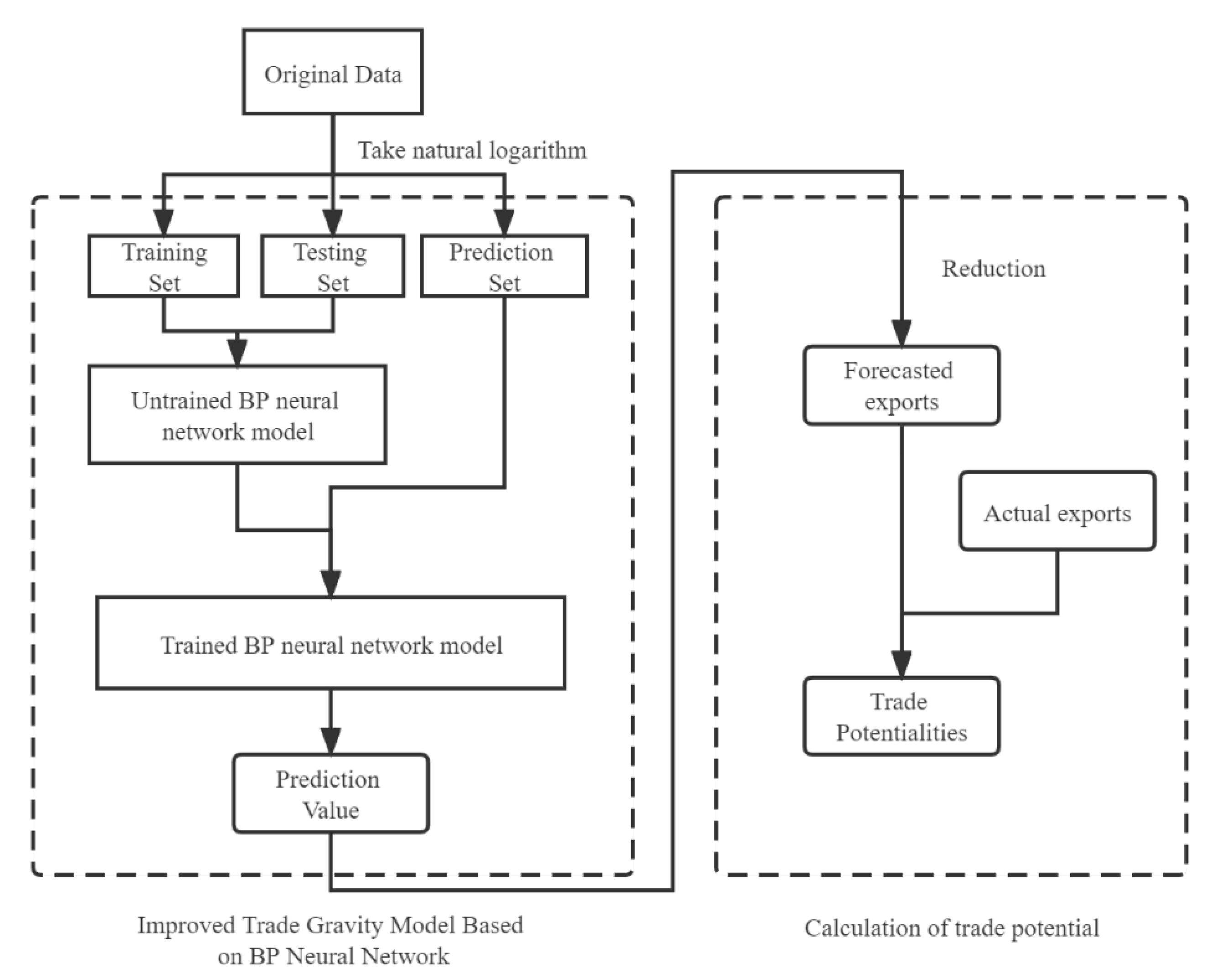
This paper mainly involves two research methods, the trade potential calculated based on the trade gravity model and BP neural-network-improved trade gravity model, and their applications are shown in Figure 3.

The two research methods are described in detail in the following two subsections.

3.1.1. Trade Potential Calculated Based on the Trade Gravity Model

(1) Trade potential

Potential refers to a capacity that exists but that has not been realized, while trade potential refers to the potential of one country to export more goods to another country. Referring to the way Shuai [14] and Batra [15] measured trade potential, in this paper, trade potential is measured by the ratio of the actual value of trade between the two countries to the theoretical estimate, as shown in the following Equation:

$$A=\frac{EX{P}_{ijt}}{E{V}_{ijt}}$$

(1)

where A is the ratio measuring trade potential, EXP_ijt refers to the actual value of a country’s exports from country i to country j in period t, and EV_ijt refers to the theoretical value of a country’s exports from country i to country j in period t. There are two main methods for assessing trade potential A: One uses 1 as the dividing line and considers that if trade potential A is greater than 1, there is trade excess and new competition points need to be created to promote trade, and if A is equal to 1, the current trade has achieved equilibrium and the trade capacity is fully utilized and there is no excess. If trade potential A is less than 1, it is considered that there is a possibility of exporting more goods; i.e., the trade potential has not been realized. Another method uses 0.8 and 1.2 as markers to classify the trade potential, with less than 0.8, within the range of 0.8 to 1.2, and more than 1.2 corresponding to “great potential”, “growth potential”, and “limited potential”, respectively. In this paper, the second classification is used to measure trade potentials according to the research study’s objectives.

(2) Traditional gravity model estimates the theoretical value of exports

The most popular method for calculating the theoretical estimates used in the academic community is the trade gravity model. The trade gravity model is derived from the Newtonian model of gravity in physics, which was first proposed by Tinbergen [27] and Poyhonen [28], which can be expressed by the following equation:

$$EV=G{S}_i{M}_j{\theta }_{ij}$$

(2)

where EV is the value of exports from one country to another, M_j represents all importers’ specific factors that constitute the total demand on the importing side (this component includes the GDP, population, etc., of the importing country). S_i denotes the exporters’ specific factors that relatively constitute the volume of exports that exporters can supply. G is a variable, such as the level of trade liberalization, that is not dependent on either exporting country i or importing country j. θ represents the inverse of the bilateral trade cost, which includes, among other things, the distance between the exporting and importing countries. Usually, multivariate trade resistance θ is denoted as $\theta =lnd\times \exp \left(\beta Dummy\right)$, where lnd is the logarithm of the distance between the exporting and importing countries; Dummy denotes one or more dummy variables related to bilateral trade costs, such as whether by a common border, etc.; and β denotes the correlation coefficient of the dummy variable.

The trade gravity model can be estimated by taking the logarithm to obtain the log-linear estimating equation, and it can be estimated using OLS, etc. The estimating equation can be expressed as follows:

$$lnE{V}_{ijt}={\beta }_0+{\beta }_{1}lnG+{\beta }_{2}ln{S}_i+{\beta }_{3}ln{M}_j+{\beta }_{4}ln{\theta }_{ij}+{\epsilon }_{ijt}$$

(3)

where β₀ denotes the intercept of the model and β_n denotes the correlation coefficient of the nth dependent variable. Furthermore, the gravity model can be extended by adding more variables to give the model more explanatory power, such as Linnemann [29], who first introduced the population factor into the basic gravity model, and Bergstrand [30], who further added the per capita income and exchange rate. Combining the research objectives and computational availability of this study, a total of seven independent variables, such as the population size of the importing and exporting countries, were selected as Mi and Si in Equation (2) to fit the logarithm of the export value. In this paper, multivariate trade boycott is estimated by means of three variables of distance between two countries and whether they are in the same tariff agreement, with import and export over whether they are in WTO or not. The meanings and attributes of each variable are shown in

Table 3. Variable meaning and attribute.

Variables	Specific Meaning	Attribute
Dependent variable
lnEV	Natural logarithm of export value (US dollars)
Independent variable
lnGDPi	Natural logarithm of exporters’ GDP (2015 constant USD)	Si
lnGDPj	Natural logarithm of GDP of importing countries (constant 2015 USD)	Mi
lnDIS	Natural logarithm of the distance between two countries (KM)	θ
RTA	Dummy variable, whether in the same tariff agreement	θ
WTOi	Dummy variable, whether the exporting country is a member of the World Trade Organization	θ
WTOj	Dummy variable, whether the importing country is a member of the World Trade Organization	θ
lnTPi	Natural logarithm of the total population of the exporting country	Si
lnTPj	Natural logarithm of the total population of the importing country	Mi
LnPCi	Natural logarithm of PV energy generation capacity (MW) plus 1 in the exporting country	Si
lnPCj	Natural logarithm of PV energy generation capacity (MW) plus 1 in the importing country	Mi

Source: determined by the authors based on study objectives and data availability.

, and the descriptive statistics of each variable are shown in

Table 4. Descriptive Statistics.

VARIABLES	(1)	(2)	(3)	(4)
	Mean	sd	Min	Max
lnEV	15.72	3.247	2.565	22.95
lnGDPi	29.25	0.833	27.82	30.51
lnGDPj	23.97	2.357	17.15	30.69
lnDIS	9.017	0.498	6.862	9.868
RTA	0.0909	0.287	0	1
WTOi	0.955	0.208	0	1
WTOj	0.793	0.405	0	1
lnTPi	21.01	0.0329	20.96	21.07
lnTPj	15.52	2.143	9.217	21.04
LnPCi	1.773	2.392	0	11.21
lnPCj	7.577	3.077	3.512	12.63

Source: Authors’ calculations.

.

3.1.2. BP Neural Network Improved Trade Gravity Model

BP neural network is a multilayer forward neural network based on an error backpropagation algorithm. Since the transfer function of neurons in the BP neural network is usually a Sigmoid-type differentiable function, it can realize any nonlinear mapping between the input and output; thus, it has wide applications in prediction, risk evaluation, adaptive control, etc.

The main structure of a BP neural network consists of one input layer, one or more hidden layers, and one output layer. Each layer consists of several neurons (nodes), and the output value of each node is determined by the input value, action function, and threshold value. The learning process of the network includes two processes: the forward propagation of information and backward propagation of error.

In the forward propagation process, the input information is transmitted from the input layer to the output layer through the implicit layer, and the output value is obtained after the action function’s operation and compared with the expected value. The output, Oj, of a neuron, j, on the implicit and output layers of the BP neural network is determined by the following equation:

$$O_j=f_j\left(Ne{t}_j\right)=f_j\left({\displaystyle \sum }{w}_{ij}{x}_i+{\theta }_j\right)$$

where f_j denotes the excitation function corresponding to neuron j, and the most used one is the Sigmoid function. θ_j denotes the threshold value of neuron j; x_i denotes the individual inputs to neuron j; w_i denotes the connection weights of the corresponding inputs and neuron j.

In the backpropagation process, the error between the output and the desired value is returned along the original connection path, and the error is reduced by modifying the weights of the neurons in each layer, layer by layer, and so on until the output meets the accuracy requirement. This process requires the use of optimization algorithms to adjust the network’s parameters so that the error between the output and the desired value of the neural network is minimized. The error metric used in this study is the mean square error (MSE) and the optimization algorithm is the Broyden–Fletcher–Goldfard–Shanno (BFGS) method.

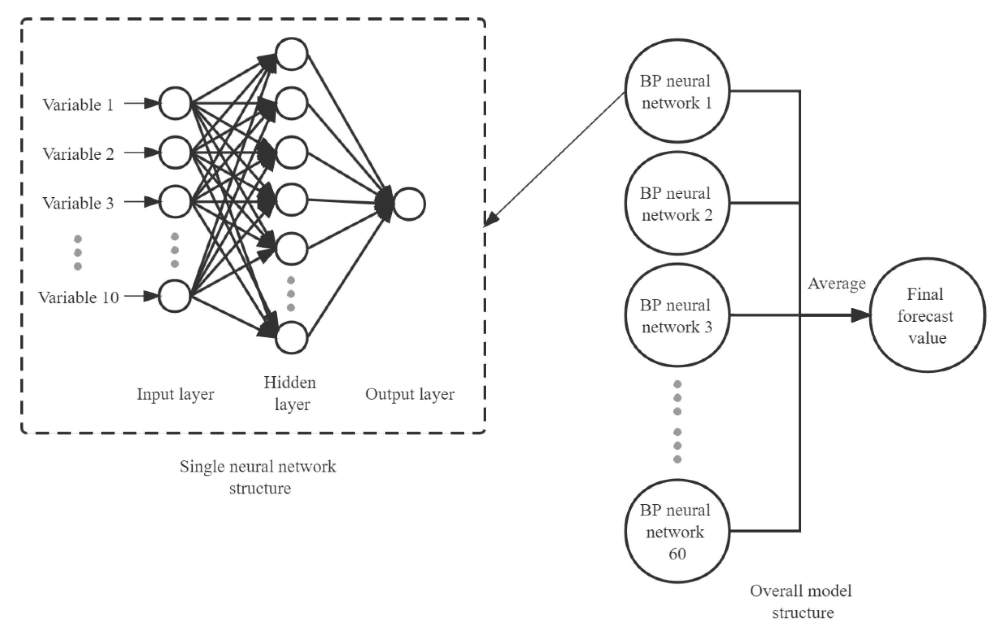
Unlike the previous body of literature [23,24], the model used in this study consists of a composite of 60 neural networks. The composite approach is to train several neural networks simultaneously using the same data set, to obtain several different neural networks and input the prediction set data into them separately, and finally to average the prediction values output from all neural networks as the final prediction result. This approach can reduce the randomness caused by the difference in the initial neuron settings of a single neural network and the difference in the solution paths of the local optimal solutions, resulting in smaller errors and higher robustness. In the single BP neural network used in this study, the input layer contains 10 neurons, the hidden layer contains 21 neurons (the number of neurons is calculated by the empirical formula n₁ = 2m + n, where n₁ is the number of neurons in the hidden layer, m is the number of neurons in the input layer, and n is the number of neurons in the output layer), and the output layer contains 1 neuron. The overall model structure is shown in Figure 4.

3.2. Data Sources

In this paper, 14 countries in RCEP, except China, were selected as the forecast sample, and the time period involved is 2000–2021, with a total of 308 trade data used as the forecast set. The selected time period covers the major events in the development of China’s PV industry, such as the revision of the Renewable Energy Law in 2010, the decreasing cost of renewable energy generation products, the 12th Five-Year Plan, the 13th Five-Year Plan to develop the renewable energy industry, etc. At the same time, this paper collects a total of 3302 pieces of PV product export data from China relative to various countries from 2000 to 2020, which are used as the training set and test set. The PV products studied in this paper include 17 products with the following HS codes: 700991, 700992, 711590, 730890, 732290, 721090, 830630, 841280, 841919, 841990, 850239, 850440, 854140, 900190, 900290, 900580, and 901380. In this paper, the data on whether the countries’ are spacing belong to WTO or not and whether they are in the same tariff agreement were obtained from the CEPII-BACI database, the PV energy generation capacity is obtained from International Renewable Energy Agency IRENA, the GDP and population numbers of each country are from World Development Index WDI, and the trade data between countries are from United Nations trade database UN Comtrade.

4. Model Building and Prediction Results

4.1. Model Building

This paper relies on MATLAB 2022a to implement BP neural networks.

(1) Parameter configuration

The BP neural network needs the correct configuration of learning rate η and system error ε to achieve the balance of training speed and error convergence. In this paper, we use the pieced-together trial method to first determine a smaller learning rate and system error for training and gradually increased the learning rate or system error if it fails to converge within the specified number of training attempts. After several attempts, this paper finally determines the learning rate to be 0.01, and the system error is set to 0.0001.

(2) Training and testing phase

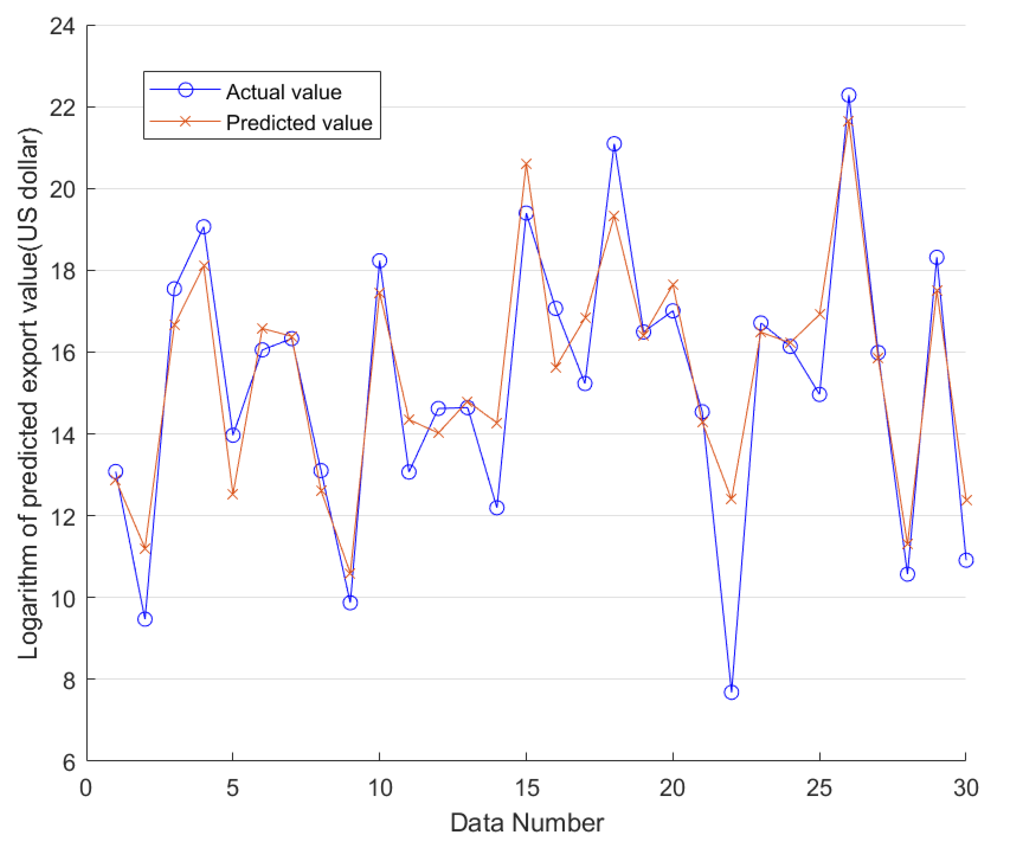
For the 3302 export data covering China’s exports to various countries around the world from 2000 to 2020, this study randomly selected 30 as the validation set to initially judge the model’s performance, and the remaining portion was used as the training set to train the neural network. In this study, 60 neural networks with a network structure of 10 × 21 × 1, a learning rate of 0.01, and a systematic error of 0.0001 were trained based on the BP algorithm, and the final model was obtained by using the average of the predicted values; the model was used to make predictions on the test set, and the prediction results are shown in Figure 5.

The mean square error (MSE) of the prediction results was 1.8132, the root mean square error was 1.3465, and the correlation coefficient R² was 0.8393. With the exception of a few samples with large differences between the actual and predicted values, most predicted values were similar to the actual values, and the model could be initially judged to have high accuracies.

4.2. Forecast Results

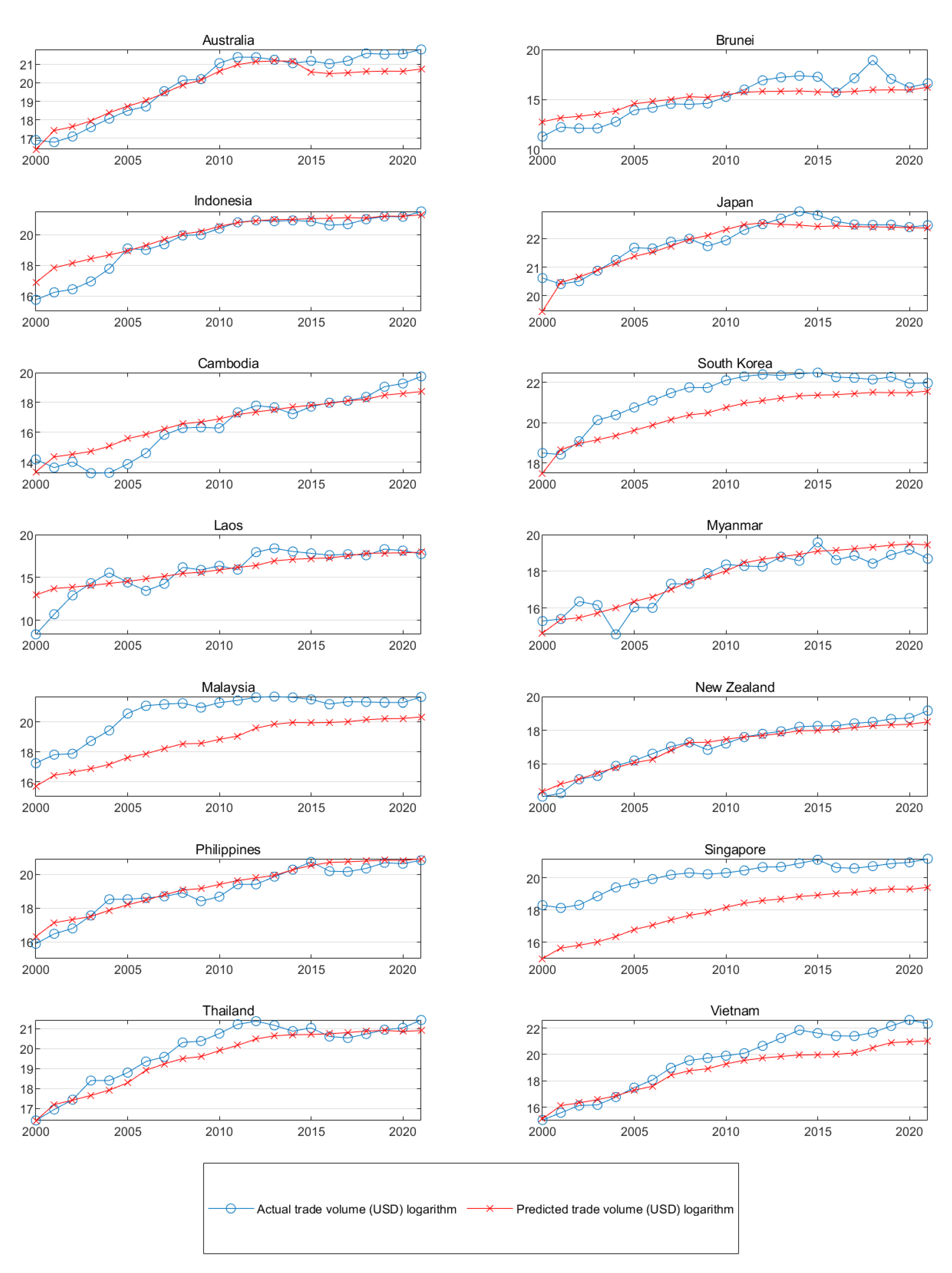
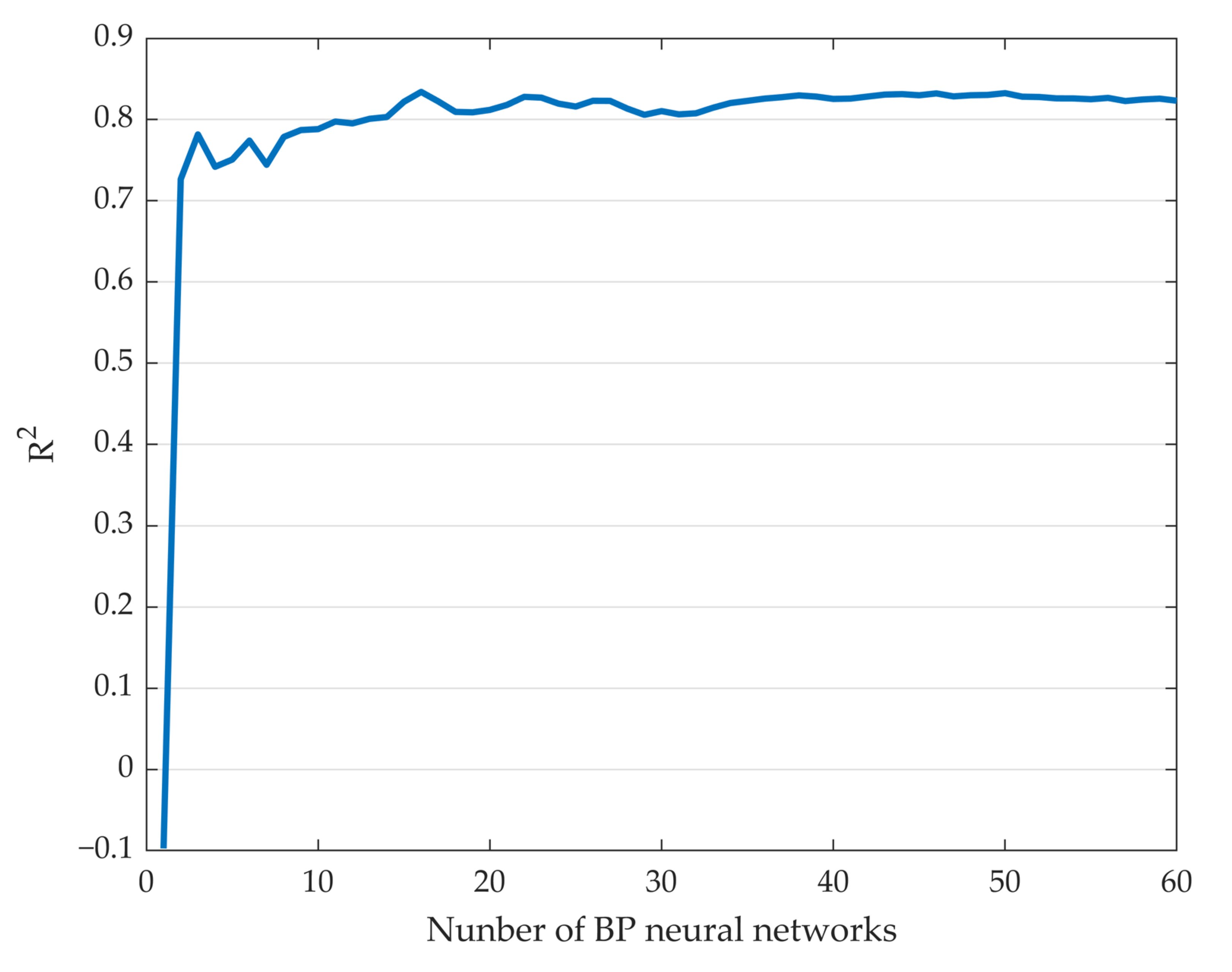
In this paper, we further input the prediction set data into the model to predict the export value of PV products from China to 14 RCEP countries, and the prediction results are shown in Figure 6. Figure 7 shows the changing processes of R² with the increase in the number of neural networks.

The mean absolute error (MAE) of this prediction is 0.7917, the mean absolute percentage error (MAPE) is 4.3587%, and the mean absolute percentage error (SMAPE) is 4.4041%. The mean square error (MSE) is 1.2274, the root mean square error (RMSE) is 1.1079, and the correlation coefficient R² is 0.8232. To further illustrate the improvement of the accuracy of BP neural network on the prediction results, the corresponding linear regression model, fixed effect model, and random effect model were built using the same data set to make comparisons with the BP neural network.

The POLS model used for comparison is described as follows:

$$\begin{array}{c}lnE{V}_{ijt}={\beta }_0+{\beta }_{1}lnGD{P}_{it}+{\beta }_{2}lnGD{P}_{jt}+{\beta }_{3}lnDI{S}_{ij}\\ +{\beta }_{4}RTA+{\beta }_{5}WT{O}_{it}+{\beta }_{6}WT{O}_{jt}+{\beta }_{7}lnT{P}_{it}+{\beta }_{8}lnT{P}_{jt}+{\beta }_{9}lnP{C}_{it}+{\beta }_{10}lnP{C}_{jt}+\epsilon \end{array}$$

where β₀ is the intercept term of the model, and β₁–β₁₀ is the slope term of each variable used in this study. ε denotes the error term. i denotes a different individual, while t denotes a different period.

The random effects model is described as follows.

$$\begin{array}{c}lnE{V}_{ijt}={\beta }_0+{\beta }_{1}lnGD{P}_{it}+{\beta }_{2}lnGD{P}_{jt}+{\beta }_{3}lnDI{S}_{ij}\\ +{\beta }_{4}RTA+{\beta }_{5}WT{O}_{it}+{\beta }_{6}WT{O}_{jt}+{\beta }_{7}lnT{P}_{it}+{\beta }_{8}lnT{P}_{jt}+{\beta }_{9}lnP{C}_{it}+{\beta }_{10}lnP{C}_{jt}+{\epsilon }_{it}\end{array}$$

The fixed effects model is described as follows:

$$\begin{array}{c}lnE{V}_{ijt}={\beta }_0+{\beta }_{1}lnGD{P}_{it}+{\beta }_{2}lnGD{P}_{jt}+{\beta }_{3}lnDI{S}_{ij}\\ +{\beta }_{4}RTA+{\beta }_{5}WT{O}_{it}+{\beta }_{6}WT{O}_{jt}+{\beta }_{7}lnT{P}_{it}+{\beta }_{8}lnT{P}_{jt}+{\beta }_{9}lnP{C}_{it}+{\beta }_{10}lnP{C}_{jt}+{\mu }_j+{\epsilon }_{it}\end{array}$$

where μ_j denotes the fixed effect of importing country j.

The comparison’s results are shown in

Table 5. Error comparison between linear regression and the BP neural network.

Group	Indicators	Value
POLS	MAE	1.0809
	MAPE	8.3005%
	SMAPE	7.8089%
	MSE	2.3972
	RMSE	1.5483
	R2	0.7733
BP Neural Network	MAE	0.7917
	MAPE	4.3587%
	SMAPE	4.4041%
	MSE	1.2274
	RMSE	1.1079
	R2	0.8232
Random effects	MAE	1.1071
	MAPE	8.3456%
	SMAPE	7.9924%
	MSE	2.4981
	RMSE	1.5805
	R2	0.7654
Fixed effects	MAE	1.4083
	MAPE	10.0955%
	SMAPE	11.4588%
	MSE	3.5577
	RMSE	1.8862
	R2	0.7282

Source: Authors’ calculations.

.

A comparison of the linear regression and BP neural network estimation errors from Figure 5 and Table 2 shows the following.

(1) All four models have a high R², indicating that all four models have acceptable prediction accuracies, but the overall accuracy of the BP neural network is higher, indicating that the neural network model is able to learn the information contained in the data species more fully and has better prediction abilities for new samples.

(2) BP neural networks have the lowest MSE and RMSE values, indicating that they have smaller confidence intervals for the same confidence level; i.e., they have more accurate prediction accuracies and stronger robustness.

(3) As the number of neural networks increases, the final prediction accuracy value will converge to a higher value. This indicates that the method of averaging the predicted values of multiple neural networks can improve the accuracy of predictions and avoid the uncertainty caused by the prediction of a single model.

4.3. MIV Analysis

After training the BP neural network, the importance of each variable in the BP neural network is further analyzed by MIV analyses, which include adding or subtracting 10% from the original value of each independent variable in training sample T to form two new training samples, T₁ and T₂, and calculating the simulation results, R₁ and R₂, by using samples T₁ and T₂. 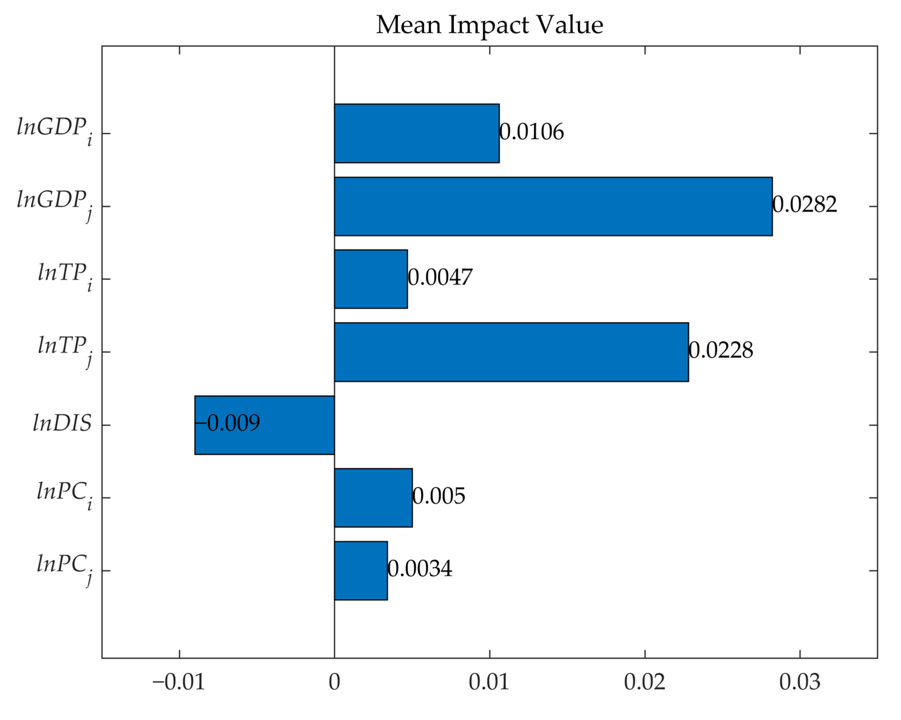The difference between R¹ and R² is the impact value (IV) of the change in the independent variable, and the mean value of IV (MIV) is the result of averaging IV for each case. MIV reflects the degree of influence of a variable on the output’s results in the model. In the neural network model constructed in this paper, the overall MIV of a variable is obtained by averaging the MIV of 60 neural networks on that variable. The three dummy variables (RTA, WTOi, and WTOj) used in this paper will not be included in the analysis because it is not economically meaningful to increase or decrease the original value of the dummy variables by 10%. The final measured MIV values of each indicator are shown in Figure 8.

The results of the MIV analysis show that the GDP of the exporting country (i.e., China), the GDP of the importing country, and the population are three factors that have the greatest impact on the output of the neural network (i.e., the predicted trade volume), and all three factors have a positive impact on the output. The population of the exporting country and the PV capacity of both importing and exporting countries have a small and positive effect on the output structure, while the distance between the two countries has a small negative effect on the network’s output.

5. Trade Potential Analysis

Furthermore, this study calculated the trade potential of PV products by country for each year based on the predicted value of China’s exports to 14 countries of RCEP by the BP neural network.

5.1. Trade Potential Trends in 2021

This study first focuses on the latest trend of the trade potential of Chinese PV products to RCEP countries, and the table of trade potential values for each country can be calculated based on the prediction results of the BP neural network, as shown in

Table 6. China’s trade potential in PV products to RCEP countries in 2021.

Year	Country	Exports (USD Million)	Trade Potential
2021	Singapore	1584.89	5.881
2021	Malaysia	2521.38	3.720
2021	Vietnam	5056.79	3.711
2021	Australia	2955.41	2.885
2021	Cambodia	376.96	2.754
2021	New Zealand	210.88	1.948
2021	Thailand	2032.54	1.702
2021	Korea	3501.43	1.490
2021	Brunei	16.25	1.465
2021	Indonesia	2195.04	1.241
2021	Japan	5700.29	1.103
2021	Philippines	1118.97	0.917
2021	Laos	50.12	0.810
2021	Myanmar	131.00	0.473

Source: Author’s calculations.

.

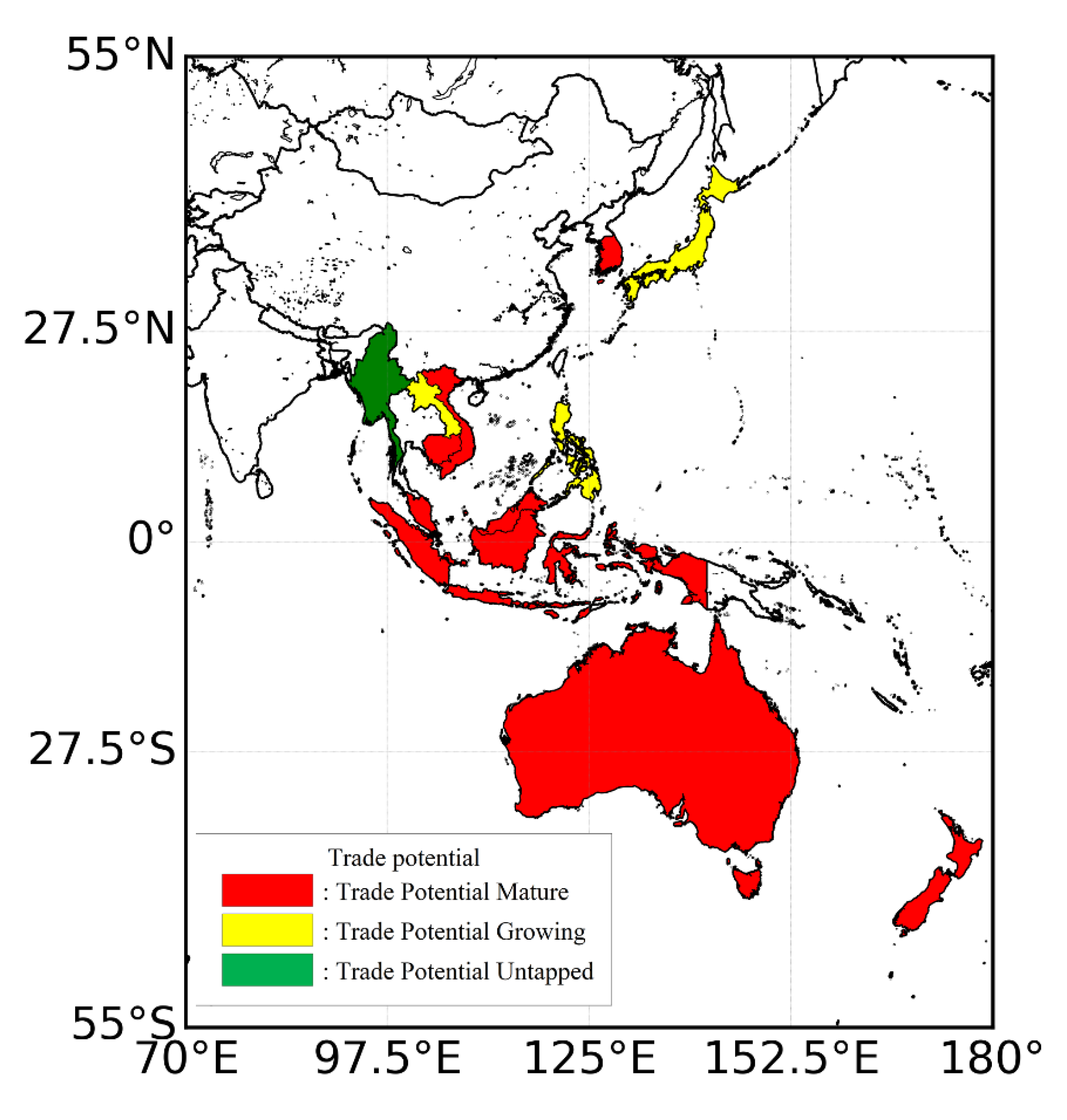
Based on the aforementioned classification, this paper further classifies RCEP14 countries in 2021 into “high potential”, “growing potential”, and “limited potential” based on their trade potential. Three types of countries are identified. The final result is 1 country with “great potential”, 3 countries with “growth potential”, and 10 countries with “limited potential”, as shown in

Table 7. China’s PV product export potential to RCEP countries in 2021 divided.

	Type of Trade Potential
Region	Great Potential	Potential Growth	Limited Potential
East Asia
			Korea
		Japan
Oceania
			New Zealand
			Australia
Southeast Asia
			Brunei
		Philippines
			Thailand
	Myanmar
			Malaysia
			Indonesia
			Cambodia
		Laos
			Singapore
			Vietnam
Total	1	3	10

Source: Author’s calculations.

.

For the purpose of analyzing the trade potential of Chinese renewable energy products in RCEP countries in 2020 and finding potential markets, this paper further marks the trade potential types of 14 RCEP countries, except for China on the map, and the results are shown in Figure 9.

The following observations were observed.

(1) In general, China’s trade relations with RCEP countries have been relatively mature. Most RCEP countries’ trade potential is of the limited potential type, while there are fewer RCEP countries with growing potential and huge potential. This may reflect that the previous path of relying on market capacities to expand PV exports has come to an end, after which China needs to create new competitive points via innovation and other means to promote the further growth of PV exports.

(2) For the East Asia region, China’s trade potential for PV products is more limited. Due to closer proximity, larger economies, and longer-term trade ties, China’s PV imports to South Korea and Japan reach USD 350 million and USD 570 million in 2021, making them the third and highest importers of Chinese PV products among RCEP countries. However, if China’s PV exports to South Korea and Japan are to expand further, new competition is needed to increase their trade potential.

(3) For the Oceania region, China’s PV product trade potential has been very well developed. New Zealand and Australia both belong to the limited potential category, and it is reasonable to assume that China’s PV exports to these two countries will stabilize if there are no exogenous factors such as policy or technological innovation changes.

(4) China’s trade potential for PV products varies greatly among Southeast Asian countries, but overall, the trade potential has been more fully exploited. Countries with high trade potential include Myanmar, Philippines, and Laos, which have long-standing trade ties with China and are closer to China, and they are also less latitudinal in position and richer in solar energy resources; these countries have hopes of establishing closer trade ties with China for PV products.

5.2. Historical Evolution of Trade Potential 2000–2021

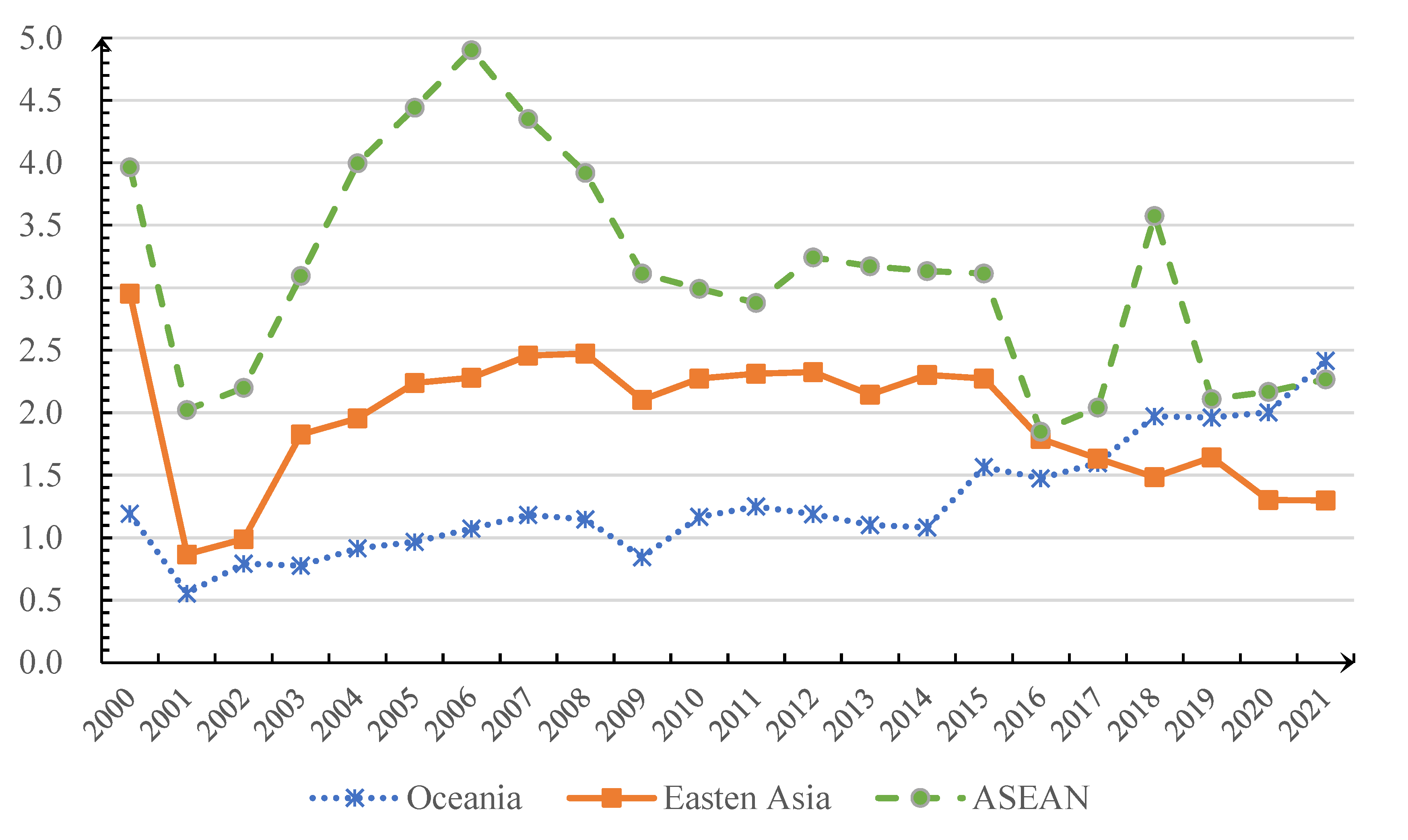
To further study the evolution trend of China’s PV product’s trade potential in RCEP countries, this study calculated the average value of China’s PV products trade potential relative to three RCEP regions’ distributions (Oceania, East Asia, and ASEAN countries from 2000 to 2021), and the results are shown in Figure 10.

It can be seen that there are obvious regional and temporal differences in the changes of China’s trade potential value of PV products relative to RCEP countries.

(1) Overall, the value of China’s trade potential with Oceania has been rising, and in 2004, the value of China’s trade potential with the region exceeded 0.8, changing from being a type with great potential to a type with growing potential, and in 2015, the trade potential with the region exceeded 1.2, exhibiting a type with limited potential. China’s trade potential with East Asia increased first and then declined, and in 2003, China’s trade potential with the region increased rapidly to 1.8, becoming a type with limited potential; in subsequent years, its trade potential remained above 1.2. China’s trade potential with Southeast Asia, on the other hand, increased and then fell, and then it slowly increased again. In all years, China’s trade potential with this region is above 1.2, which is a type with limited potential. The possible reasons for the above changes in trade potential are that China’s deepening trade ties with the Oceania region has led to a fuller trade potential with Oceania, which has led to an increasing trade potential, while China’s innovation in photovoltaic technology and the rapid economic development of the Asian region after 2006 and 2015 led to increasing trade potentials with East and Southeast Asia.

(2) In 2001, the year of China’s accession to the WTO, the value of China’s trade potential relative to all three regions declined significantly, indicating that the event of China’s accession to the WTO gave China the opportunity to engage in larger-scale trade with respect to PV products in the RCEP region, which led to a rapid increase in trade potential. At the same time, the impact of the event on different regions exhibited more obvious heterogeneity. China’s accession to the WTO has had the most significant impact on the trade potential of East and Southeast Asia, while the impact on the Oceania region is lower.

(3) There are two extremes in the time series of changes in trade potentials in Southeast Asia that are worthy of attention. The year 2006 experienced a rapid increase in trade potential with Southeast Asia, while China’s trade potential with other regions began to decline for the first time after its accession to the WTO during the impact of the 2008–2009 financial crisis, which may be related to the boom in the construction of renewable energy facilities in the region. In 2018, there was a significant decline in trade potentials with Southeast Asia, and the sharp increase in this average value was mainly influenced by the extreme value of Brunei, for which its PV imports from China jumped to USD 0.16 billion in that year, which is six times higher than in 2017, bringing the value of its trade potential to 20.04.

6. Conclusions and Policy Recommendations

In the above analysis, this study uses the BPNN-improved trade gravity model to measure the trade potential of Chinese PV products relative to RCEP countries. The three main results obtained from the analysis of this paper are as follows.

(1) The BP neural network is a more effective estimation method than the use of traditional pooled regression, fixed effects, and random effects, and the combination of multiple neural networks for prediction can lead to more robust and accurate results. In this study, the four models of the BP neural network, mixed regression, fixed effects, and random effects were constructed using the same data set, and their goodness-of-fit was compared using three values comprising MSE, RMSE, and R². It was found that the BP neural network was the most accurate estimation. Moreover, the estimated R² converges to a high level by combining multiple neural networks.

(2) China’s trade potential in PV products with RCEP countries is relatively mature, and the trade potential of most countries is relatively limited, but the scale of PV product trades between China and Japan, the Philippines, Myanmar, and Laos may still be further deepened. The trade potential values measured in this study show that China has the highest trade potential with Myanmar, which belongs to the type of countries with great potential, while Laos, the Philippines, and Japan belong to the type of countries with growing potential, and the trade potential can still be further developed.

(3) China’s trade potential for different regions in the RCEP agreement changed historically with respect to different processes, with China’s trade potential for the Oceania region decreasing, while its trade potential for the East and Southeast Asia regions increased in recent years. The trade potential values measured in this study show that after China’s accession to the WTO in 2001, the type of PV product trade potential for the Oceania region was transformed into a limited potential type in 2015, while for the East Asia region, this transformation occurred in 2003, and the type of trade potential for the Southeast Asian countries has been the limited potential type.

Although the latest data show that China’s trade potential in most of the regions covered by the RCEP agreement has been fully exploited, the trade potential trend in East and Southeast Asia has not disappeared, but rather, it has become more pronounced. This paper believes that with the operation of the RCEP agreement and China’s opening-up policy, the trade and cooperation between China and other countries of the RCEP agreement in the field of photovoltaic products and even the entire renewable energy field will be more in depth and make more contributions to the world’s shift to green energy.

With such an outlook on renewable energy cooperation, the policy recommendations given in this paper are as follows.

(1) We further recommend promoting the implementation of the RCEP agreement and breaking the unfavorable factors of trade among the RCEP member countries. This paper finds that under the current conditions, China’s trade potential for PV products relative to other RCEP countries has been fully utilized, and the trade potential relative to each RCEP region has been at a low level in recent years. The bilateral trade flow lacks a breakthrough point, and the bilateral trade cost reduction induced by the operation of RCEP is likely to become a new growth point for China’s renewable energy trade with RCEP countries. Therefore, China should actively implement the contents of the RCEP agreement, break trade disadvantages, and reduce the transaction costs by effectively reducing the tariff preference threshold and strengthening the supply chain of the regional industry chain in order to promote the trade cooperation of renewable energy products in the region.

(2) We recommend actively expanding China’s trade relations with RCEP countries for PV products and strengthening cooperative relationships via differentiated strategies. The results of this paper show that China’s trade potential with each country varies widely, and although China’s overall trade flows are saturated, China still has high trade potential with some countries, such as Myanmar. China should take advantage of the favorable trade conditions provided by RCEP to strengthen ties with high-potential and growth countries (e.g., Myanmar, Japan, and the Philippines) to further tap their potential, while consolidating ties with countries with limited potential. In future, China’s PV exports should be focused on high potential and growth countries.