Abstract
Energy planning has become more complicated in the 21st century of sustainable development due to the inclusion of numerous standards such as techno-economic, and environmental considerations. This paper proposes multi-criteria sustainable planning (MCSP) based optimization approach for identifying DGs’ optimal allocations and rating powers. The main objectives of this paper are the reduction of the network’s total power loss, voltage profile improvement, energy loss saving maximization, and curtailing environmental emissions and water consumption to achieve Sustainable Development Goals (SDGs 3, 6, 7, 13, and 15) by taking the constraints into consideration. Different alternatives are evaluated across four aspects of performance indices; technical, cost-economic, environmental, and social (TEES). In terms of TEES performance evaluations, various multi-criteria decision-making (MCDM) approaches are used to determine the optimal trade-off among the available solutions. These methods are gaining wide acceptance due to their flexibility while considering all criteria and objectives concurrently. Annual energy loss saving is increased by 97.13%, voltage profile is improved to 0.9943 (p.u), and emissions are reduced by 82.45% using the proposed technique. The numerical results of the proposed MCSP approach are compared to previously published works to validate and may be used by researchers and energy planners as a planning tool for ADN schemes.
1. Introduction
In recent years, with rising energy demand, conventional networks are becoming more complicated, hazardous, uneconomical, and with significant power losses [1]. The rate of development of any society is measured by its energy consumption. Due to industrial, economic, and social changes, load demand is rapidly increasing. As a result, energy resources are a major concern worldwide. The problem is finding the most efficient and cost-effective way to provide the required power [2]. Distributed generation (DG) refers to small-scale power generation that happens at or near the load center. The size of a DG unit can range from a few kilowatts to a few megawatts. Solar photovoltaic, wind turbines, small hydro, biomass, gas turbines, and other DG technologies are currently in use. DGs are responsible for injecting active and reactive powers into the distribution networks (DN). Adoption of DG units benefits both electric utilities and consumers [3]. Power flows in a uni-direction from the radial distribution network (RDN) to the load centers. However, the integration of small, medium, and large sizes of DGs, transforms their passive structure into an active distribution network (ADN) with multi-directional power flows [4].
The development of DG technologies, the challenges of constructing a new transmission line, the increase in consumer demand, the economics of the electric power market, and the impact of climate change have all aroused interest in DG allocation throughout DN. The depletion of fossil fuel sources and continued progress in the sector of non-conventional ones have prompted utilities to switch to DGs [5]. The distribution system has the highest percentage of power losses, around 70% owing to its low voltage level and high current carrying capacity [6,7]. The primary goal of DG integration is to reduce power losses and improve voltage profiles, which in turn, increases the overall efficiency of the power system [8]. In terms of real and reactive power delivery capability, DGs can be categorized as follows [9]:
- Type-I: DGs injecting only active power.
- Type-II: DGs injecting only reactive power.
- Type-III: DGs injecting both active and reactive power.
- Type-IV: DGs injecting active but consuming reactive power.
Due to national and international policies aimed at increasing the share of renewable energy sources (RES) and highly efficient micro-combined heat and power (CHP) units in order to reduce greenhouse gas (GHG) emissions and mitigate global warming [10]. Currently, non-renewable energy (mostly fossil) meets over 80% of the global energy demand, leaving an imprint on land through resource extraction, conversion, and infrastructure. Similarly, the growth of RES such as biomass, geothermal, hydro, solar, and wind have land-related repercussions, however, these vary in scale and form. Environment-friendly technologies are being promoted by governments as a means of achieving sustainable development goals (SDG 7) and enhancing global energy security. Distribution network operators (DNOs) are working hard to harness this momentum in order to provide network operational benefits such as increased voltage stability, system dependability, loadability, and decreased losses as a result of successful DG implementation [11].
The use of DGs improves power quality and reliability, as well as lower generating costs and carbon emissions [12]. Furthermore, advances in compact generators, uninterruptible power supplies (UPS), storage devices, and power electronic devices have accelerated the usage of DGs in power plants [13]. DG units give savings on fuel investment and thus minimize the electricity prices and also increase the system’s voltage stability and voltage stability margin [14]. Utility firms may also use these generation technologies to diversify their energy matrix and turn electric power networks into autonomous and intelligent systems [15]. The integration of DGs into the DN has grown rapidly as a result of technical, economical, environmental, and social benefits, as illustrated in Figure 1.
Figure 1.
Benefits of DG integration.
In DNs, traditional asset optimization methodologies focused on finding an alternative with the lowest possible cost. However, such methods lack a solution that is applicable to all of the required rubrics. Analytical approaches, such as analytical method and efficient analytical (EA) methodology, were thoroughly articulated in a mathematical formulation for the power system to investigate the impacts of the injected DGs power on the performance of the power system [16,17]. However, some analytical techniques were ineffective in determining the best size and position for multiple DGs [18].
To optimize the benefits of DG installation, many authors have proposed various optimization methodologies and objective criteria for the best locations and sizing of DGs in the distribution system. Different optimization-based strategies have been used to overcome the limitations of the numerical methods. The most often utilized methodologies include genetic algorithms (GA), particle swarm optimization (PSO), and multi-objective algorithms. In [19], researchers presented a multi-objective, modified honey bee mating optimization (HBMO) method for DG siting and sizing to minimize power loss, generation cost, voltage deviation, and emissions. In order to reduce power losses and improve voltage profile and stability, a hybrid GA-PSO-based technique for optimal DG allocation in IEEE 33-bus and 69-bus systems has been described [20]. To reduce power losses, modified teaching–learning-based optimization method (MTLBO) was used to find the optimal locations and size of DGs in 69-bus, and 119-bus of RDN [21]. Multi-objective particle swarm optimization (PSO) for DG placement in IEEE 33-bus has been used for power loss reduction, voltage profile enhancement, and economic analysis [22]. On a standard 10 kV distribution system, an improved harmony search algorithm (IHSA) has been implemented for non-dispatchable DGs allocation [23]. To reduce power loss and loss expenses in IEEE 33 and 69-bus radial systems, the intersect mutation differential evolution (IMDE) algorithm was used to find the optimal positions and sizes of DGs and SCs [7]. To reduce power losses and improve voltage profiles and to increase net saving, ant lion optimization algorithm (ALO) was presented for optimal DG allocations and sizing in 33-bus and 69-bus radial distribution systems [24]. Water cycle algorithm (WCA) has been proposed to find the optimal positions and size of DGs and CBs to achieve techno-economic, and environmental benefits [25]. Lightning attachment procedure optimization (LAPO) was used to find the proper location of renewable energy resources (wind and solar PV) in a 118-bus system for loss reduction while taking into account the system’s uncertainties [26]. In IEEE 85-bus distribution system with multiple load levels, the grey wolf optimizer (GWO) was used to allocate PV-based DG and DSTATCOM in terms of power loss reduction [27].
A salp swarm algorithm (SSA) has been used to locate the optimal locations and sizes of DGs and CBs in the distribution network to gain technical, economical, and environmental advantages [28]. A multi-objective Bat algorithm (MOBA) has been used to find the optimal location and capacity of DG units in 33-bus, 69-bus, and 85-bus systems to reduce the active power loss and increase the voltage stability index [29]. For optimal DG allocation, a modified adaptive genetic algorithm (AGA) was used to provide active and reactive power compensation in order to reduce network power loss and voltage drop [30]. Elephant herding optimization (EHO) was proposed to find the optimal sizing and locations of DGs in IEEE 15-bus, 33-bus, and 69-bus test systems for cost-benefit analysis [31]. An enhanced genetic algorithm (EGA) that incorporates the merits of genetic algorithm and local search was used to deploy the DGs and SCs in IEEE 33-bus, 69-bus, and 119-bus test distribution systems for the reduction of power loss and voltage deviation [32]. To boost the techno-economic benefits of DG deployment in RDN, an improved raven roosting optimization (IRRO) method was implemented [33]. The manta ray foraging optimization technique (MRFO) was used to determine the position and capacity of type one DGs in order to reduce power losses in RDN [34].
Several methods have been proposed in the literature to handle the aforementioned distribution system concerns and challenges. Based on the above literature, the best allocation of DGs in IEEE 33-bus and 69-bus distribution networks has been explored by various researchers to investigate the power loss and voltage drop problem. Some authors have looked into techno-economic parameters, while others have looked into the use of DGs for both techno-economic and environmental indices. It has been observed that the use of DGs for technical, cost-economic, environmental, and social evaluation is quite rare. Apart from the deployment, DGs are considered in four operational scenarios; unity, 0.90 LPF, 0.85 LPF, and OPF, all of which have been found to be lacking in a single research paper. In this paper, multi-criteria sustainable planning (MCSP) approach based on efficient and nature-inspired meta-heuristic moth flame optimization (MFO) technique is used to optimally place the single and multiple DGs units into ADNs. The effectiveness and convergence of the proposed MFO are verified and compared to the marine predators algorithm (MPA) method. A multi-criteria framework considering techno-economic-environmental-social (TEES) objectives is the novelty of this research work and a pre-requisite for planners in different power scenarios for power growth and sustainability.
The main contributions and findings of this paper can be summarized as follows:
- (i)
- Evaluation with techno-economic-environmental-social performance metrics.
- (ii)
- Power loss minimization and maximization of voltage profile are considered.
- (iii)
- Studying the penetration of DGs to enhance the techno-economic and environmental challenges of distribution networks.
- (iv)
- Cost-economic analysis of adopting DGs is considered.
- (v)
- Reduction in water consumption and GHG emissions, which is essential to mitigate climate change, as set forth in SDGs.
- (vi)
- Social impacts of the penetration of DGs.
- (vii)
- Evaluation of trade-off solutions across sets of alternatives.
- (viii)
- Numerical evaluations are conducted across IEEE 33-bus and 69-bus ADNs.
- (ix)
- Validation of results with those reported in the literature as a benchmark.
The rest paper is organized as follows: Section 2 describes power flow computation, performance evaluation indices, operational constraints, and MCDM methods. Section 3 gives an overview of the optimization methods. In Section 4, numerical results are given. Finally, the conclusion and future work are presented in Section 5.
2. Problem Formulation
The power flow is analyzed using the backward/forward sweep method, which is an effective approach for calculating load flow. The suggested optimization method is applied for the optimal allocation of DGs in ADNs and the convergence rate is compared to MPA. When termination criteria are satisfied then techno-economic and environmental-social performance evaluations are performed. MCDM methods are used to determine a trade-off amongst several important criteria that are incompatible.
2.1. Power Flow Computation
The aim of this research is to determine the optimal locations and sizes of DGs in ADNs. A single-line diagram of a simple RDN system is shown in Figure 2. The backward/forward sweep method is implemented by using a set of mathematical equations as [35]:
Figure 2.
Single line diagram of RDN.
2.2. Performance Evaluation Indices
For an evaluation of the most feasible solutions using the proposed planning approach, the values related to voltage profiles and system losses, as well as other performance indices (PI), need to be considered. In this paper, four types of PI are discussed. Evaluation parameters used in this study are given in Table 1. And PI with aimed objectives is given in Table 2.

Table 1.
Evaluation parameters.
Table 2.
Performance Indices & Objectives.
2.2.1. Technical Performance Indices
The following technical indices (TI) are considered in the performance analysis:
Power Loss
By summing the losses for all branches in the distribution system, the total active and reactive power losses can be computed as:
Active power loss minimization and reactive power loss minimization are calculated as:
DG Penetration Level
It is the ratio of total DG power generation by n DGs over total load demand across nodes in a DN [36].
Voltage Profile
Voltage dips can occur at the terminal nodes of some branches. The installed DG can tackle the adjacent loads after penetration with the appropriate DG at the best position. The voltage profile of the system improves substantially.
Voltage Stability Index
The Voltage Stability Index (VSI) is calculated as [37]:
The positive value of VSI ensures the system’s safe operation.
2.2.2. Cost-Econonmic Performance Indices
The cost-economic performance analysis considers the following indices:
Cost of Energy Loss
The cost of energy loss , which is the yearly cost of energy loss, is presented by (13).
where the cost of an electricity unit is 0.06 kWh, and T is the time period in one year (8760 h) [38].
Energy Loss Saving
Cost of DG
The cost of active power DG is calculated as [39]:
The cost coefficients of are: a2 = 0, a1 = 20, a0 = 0.25. The cost of reactive power DG is calculated as [39]:
where and . The value of k is considered to be 0.75.
Cost of Annual Investment
The cost of annual investment for DG is typically proportionate to its maximum capacity. The cost of DG units varies based on their type and use. DGs are considered to operate at unity and lagging power factors in this paper and are capable of providing both active and reactive powers.
and,
where is the annualized factor, is the interest rate based on annual cost and t is DG’s service life. is the DG capacity in limits of 0.001–2 MVA, and is the cost of a DG unit. The information and assessment of the aforementioned PI can be found in [36,40].
Optimal deployment of DGs in ADN is done to achieve the techno-economic benefits. The net profit including the total costs of DGs and revenue is defined as:
2.2.3. Environmental Performance Indices
The environmental impacts of power generation are gaining traction. Renewable power plants are leading the way in terms of lowering GHG emissions, water, land management, and overall sustainable power generation. Three different environmental indicators are discussed here.
Pollution Emission
DGs produce energy with the least amount of GHG emissions as compared to traditional technologies. The public’s concern about the greenhouse effect is growing rapidly. A proper power planning model is required to carry out an energy expansion that is consistent with CO2 reduction aims.
The amount of emission for ith pollutant PEi with and without the placement of DG can be expressed as [41]:
where is the emission factor (kgCO2/kWh) of ith pollutant. n is the number of conventional plants and m is the number of DG plants.
Carbon emission factors associated with per unit of energy for the base coal power plant and other DG power plants are given in [42]. Only CO2 emissions are studied in this research since they are substantially associated positively with emissions of other pollutants and are the most extensively used energy pollutant emission indicator.
Water Consumption
Operational processes such as cooling, fuel treatment, steam production, and emission control technologies all use water in power plants. Similarly to PE [41], Water consumption (WC) with and without the employment of DG is presented as (22) and (23).
where WCF denotes the water consumption factor (gal/MWh) for jth conventional power plant and kth DG power plant respectively. This study typically focuses on cooling systems, as most of the water is used during electricity generation. WCF of DGs and conventional power plants vary substantially within and across technology categories as given in [43].
Land Use
Land management has become a major concern with the expansion of systems and DER. Non-renewable energy resources (mostly fossil) are used to meet global energy demand, leaving an imprint on land via resource extraction, conversion, and infrastructure. Renewable energy production, such as biomass, hydro, solar, geothermal, and wind, also has land implications, albeit they vary in scope and form. The amount of land used to generate one unit of energy using the various systems (spatial footprint) is expressed as:
where LUI is the land use intensity (m2/MWh). Only direct land requirements are considered in this paper, not indirect land use. Renewable-based DGs can help to alleviate land use demands while avoiding the landscape disruptions created by fossil fuels. The land footprints of energy systems vary depending on the source [44].
2.2.4. Social Performance Indices
The use of renewables reduces the usage of fossil fuels and the emissions of associated air pollutants, which have a favorable impact on human health, ultimately improving the global quality of life. There is a negative relationship between renewable energy (RE) and CO2. If favorable outcomes in the reduction of CO2 emissions are achieved, people’s behavior will improve further, resulting in a rise in RE. Individuals’ well-being and awareness might lead to a higher demand for RES. Policymakers should use a variety of policy instruments to promote societal sustainability and awareness regarding the transition to renewable-energy economies.
The performance analysis considers the following social indicators.
Life Quality
This indicator tells about how much positive change comes to the public’s life quality after the integration of DGs. The LQValue is calculated as:
where 15% is a LQ factor [39]. LQ in percentage after the deployment of DGs can be determined as:
Social Awareness
This indicator tells about awareness regarding the penetration of DGs into the electric power system. The SAValue is found as:
where 35% is a SA factor [39]. Social awareness in percentage after the installation of DGs can be determined as:
2.3. Operational Constraints
While achieving the objective functions, the system is subjected to some constraints that must be met.
2.3.1. Equality Constraints
A balance between power generation and demand, as well as power loss, should be taken into account. This can be mathematically represented as:
2.3.2. Inequality Constraints
Both bus voltages and DG size limits are inequality constraints for the simulated power system. These two limitations are mathematically represented as follows:
Voltage Constraint
The bus system voltage must be kept between Vmax and Vmin. The voltage variations in this work are set at 0.90 (p.u) and 1.05 (p.u) respectively.
DG Sizing Constraint
DG’s sizing constraints are expressed as:
DG capacity limits are set between 0.001 to 2 MVA.
2.4. Multi-Criteria Decision Making Analysis
Multi-criteria decision-making (MCDM) techniques are used to solve decision-making problems involving a set of predetermined solutions. To assess energy planning based on technical, economical, environmental, and social (TEES) aspects, MCDM methods are utilized. Different techniques have different approaches to incorporating cogent or delicate criteria. MCDM models are most adapted to achieve the optimal solution when considering numerous scenarios, factors, and limitations. This paper highlights various MCDM models that can be used to solve the core challenges that must be addressed in order to achieve sustainability goals [45]. The proposed system layout is shown in Figure 3.
Figure 3.
Proposed system layout.
In addition to main objective of deploying DGs in ADN to reduce power loss , and enhance voltage profile , other PI such as , , , , , , , and are also considered in MCSP approach for TEES evaluation. The weights for each criterion are considered biased (unequal) and calculated by AHP [46]. Selected alternatives, attributes, the priority or relevance of each attribute, and performance ratings are all included in the decision matrix. The decision matrix is shown in Table 3. The matrix consists of alternatives (for j = 1 to n), attributes (for k = 1 to m), weights considered for attributes (for k = 1 to m) and performance ratings for alternatives (for j = 1 to n; k = 1 to m). The sum of should be equal to 1 as illustrated in (34).
Table 3.
Decision matrix in MCDM methods.
Normalization matrix helps to enable a standard unified scale for measurement and analysis. The decision matrix is normalized using (35) and (36) for beneficial and non-beneficial attributes respectively.
Four different MCDM techniques are employed in this paper for evaluating performance in order to get the optimal solution.
2.4.1. Weighted Sum Method
Optimal solution among m alternatives based on n criteria are calculated as:
where, denotes the weighted sum score. The best solution is considered the one with the highest score.
2.4.2. Weighted Product Method
Based on n criteria, the optimal solution among m alternatives is calculated as:
where, indicates the weighted product score. The solution with the highest score is considered the best.
2.4.3. Technique for Order of Preference by Similarity to Ideal Solution
This technique is based on the concept of measuring the distance from two hypothetical solutions, the negative ideal solution (NIS) and the positive ideal solution (PIS). The best-chosen alternative should have the shortest geometric distance from the best solution and the longest geometric distance from the worst solution. TOPSIS process can be summarized as:
The normalized decision matrix is calculated using (39).
The weighted normalized decision matrix Xjk is calculated as:
Best PIS and worst NIS alternative for each criterion are calculated as:
The Euclidean distance is determined as:
The relative similarity of each alternative to and from the ideal solutions is determined for estimating the closeness of the available alternatives.
The best solution is the alternative with the highest Pj value.
2.4.4. VIseKriterijumska Optimizacija I Kompromisno Resenje
The VIKOR process is summarized as:
Determine the best and worst values for all beneficial and non-beneficial criterion functions.
The normalized decision matrix is calculated as:
Compute utility measure Sj and regret measure Rj as:
Now, calculates the VIKOR index.
where and v is the weight for the maximum group utility strategy, which is commonly set to 0.5 for a balanced approach. The alternative with the smallest VIKOR value is determined to be the best available solution.
3. Overview of Optimization Techniques
In this section, optimization methods are presented and analyzed to solve the optimization problem.
3.1. Moth Flame Optimization
The MFO is a bio-inspired metaheuristic optimization technique invented by Seyedali Mirjalili [47]. The major source of inspiration for this optimization is the transverse orientation navigation mechanism used by the moths. This unique moth behavior is mathematically described in order to accomplish the optimization. Despite the effectiveness of traveling in a transverse path, moths still choose to spiral around the lights. Moths actually do act in this way when they are confused by indoor lighting. This is because of the drawbacks of the transverse orientation, which make it ineffective for straight-line motion unless dealing with highly distant light sources. When approaching a man-made artificial light source, moths will seek to keep a similar angle. Because the light source is so much closer than the moon, moths that try to fly at an equal angle to it end up taking a lethal spiral flight path. A conceptual illustration of this behavior is presented in Figure 4. The candidate solutions in this population-based algorithm are assumed to be moths, and the variables represent the position of moths in space. The moths may change their positions and fly in one, two, three, or higher-dimensional space. The moth matrix [47] may be written as follows:
where n is the number of moths and d represents the number of variables or dimensions. For every moth, their fitness value is calculated and stored in an array as follows:
Figure 4.
MFO spiral path.
The population of flames is represented by a flame matrix similar to moth matrix [47]:
And the corresponding array of fitness values is given as:
Equation (56) represents the update process for the position of each moth relative to a flame.
where denotes the ith moth, for jth flame and S for the spiral/helical function. Therefore, a logarithmic spiral for the moth flight path [47] is defined as follows:
where shows the distance between the moth and the flame, b is the logarithmic shape constant, and t is the random number in [−1, 1]. It is then conceivable to visualize a hyper elliptical extending outwards from the center of the flame, within which the moth would be located. Because of the spiral equation, the moth can successfully explore and exploit the search zone by flying around the flame rather than in the space between them. Figure 5 shows the logarithmic spiral, the space around the flame, and the values of t on the curve. L is calculated as:
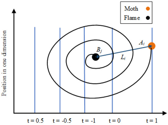
Figure 5.
MFO logarithmic spiral.
An adaptive approach [47] is used for determining the number of flames which reduces as the number of iterations increases.
where k is the current number of iterations, N for the maximum number of flames, and denotes the maximum number of iterations. MFO flowchart is shown in Figure 6 and Algorithm 1 shows the pseudo-code of the proposed MFO.
| Algorithm 1 Pseudo Code of MFO |
|
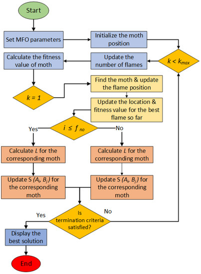
Figure 6.
MFO flow chart.
3.2. Marine Predators Algorithm
The marine predators algorithm (MPA) is a nature-inspired metaheuristic optimization approach. It is based on the relationship between the predator and the prey. Both predators and prey search for food in nature and are considered candidate solutions. MPA is based on marine predators’ diverse foraging strategies, particularly Levy flight and Brownian motion, as well as the predator-prey interaction’s optimal encounter rate approach [48].
In MPA, the initial solution is uniformly dispersed across the search space. This may be accomplished as follows:
where and are the lower and upper bound variables respectively, and is a uniform random value in the range [0 1].
Based on the theory of fittest ones survive, and the top predators in nature, are better foragers. In order to build an elite matrix (E), the top predator is recognized as the best solution. To find the prey, the E matrix array is used.
where N is the number of search agents and D is the number of dimensions. The prey matrix (P) is another matrix with the same dimension as E, in which predators change their positions. The P matrix is given in (62).
Based on the speed ratio, the MPA optimization process is separated into three phases. The three phases of this technique are depicted schematically in Figure 7.
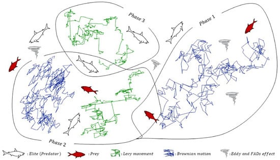
Figure 7.
MPA optimization phases [48].
3.2.1. Phase 1
This stage happens during the initial optimization rounds, where the exploration interests are explored. This stage’s mathematical representation is as follows:
while
where Brownian motion is represented by the vector , which is a vector of random numbers based on the normal distribution. Entry-wise multiplications are denoted by the symbol ⊗. Q = 0.5 is a constant number, and R is a vector of uniform random values in the range [0, 1]. The current iteration is t, while the maximum iteration is T.
3.2.2. Phase 2
When the exploration is trying to be turned into exploitation, this phase occurs in the middle of the optimization process. As a result, half of the population is designated for exploration and the other half for exploitation.
While
- First half of the population:where indicates Lévy movement and is a vector of random numbers based on the Lévy distribution.
- Second half of the population:where is an adaptive parameter that controls the predator’s step length during movement.
3.2.3. Phase 3
This occurs in the last phase of optimization, which is frequently associated with exceptional exploitation capabilities.
While
The behavior of marine predators is influenced by environmental factors. Fish aggregating devices (FADs) are an example of environmental concerns. FADs are considered local optima solutions. FADs may be expressed mathematically as:
FADs have a chance of influencing the optimization process. U is a binary vector containing zero and one array. This is accomplished by constructing a random vector in the range [0, 1] and setting the array to zero if the value is less than 0.2 and one if the value is more than 0.2. The uniform random number in the range [0, 1] is r. The bottom and top borders of the dimensions are represented by the vectors and . The random indices of the prey matrix are and .
Marine predators have an eidetic memory. After updating the current position, compare the fitness values of the current and previous positions and exchange them if the old position’s fitness is better than the current. The MPA flowchart is shown in Figure 8 and the pseudo-code is listed as Algorithm 2.
| Algorithm 2 Pseudo Code of MPA |
|
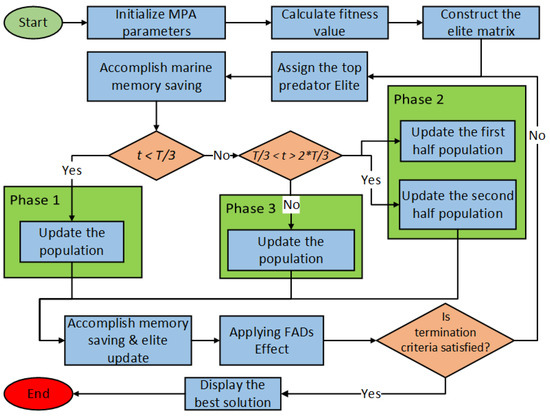
Figure 8.
MPA Flow Chart.
4. Results and Discussion
In this section, the proposed MFO has been evaluated in two IEEE benchmark DNs, including 33-bus and 69-bus systems for different scenarios along with single and multiple DGs placement. DGs types I and III are used in these test systems. The optimal size and locations of DGs have been found using the proposed technique to minimize the total power losses and to increase the magnitude of bus voltage. To evaluate the effectiveness of the proposed method, we used another marine predator optimization technique to tackle the same ODGA problem, for comparison of results and convergence. The size of the population for both optimization techniques is considered as 100. The initial values without DG integration for base cases for both test systems are summarized in Table 4. The proposed method is simulated in MATLAB 2020a environment on an Intel Core i3-4030U, 1.90 GHz processor with 4 GB RAM.
Table 4.
PI in base case without DGs (33-bus and 69-bus).
Different scenarios and cases (S/C) are considered in the studied system with multiple types of DGs (Type I and Type III).
- (S0/C0): Base case (without DG).
- (S1/C1-3): Integrating DGs at UPF.
- (S2/C1-3): Integrating DGs at 0.90 LPF.
- (S3/C1-3): Integrating DGs at 0.85 LPF.
- (S4/C3): Integrating DGs at OPF.
4.1. Test System 1
The benchmarking network IEEE 33-bus system, which is used to test and evaluate the different types of DG units is shown in Figure 9. There are 33 buses and 32 lines in this system. The total active power load (PLD) of this system is 3715 kW and the reactive power load (QLD) is 2300 kVAR, at the base values of 100 MVA and 12.66 kV. In base case S0/C0_1, total active power losses (PLoss) are 210.1 kW and reactive power losses (QLoss) are 142.4 kVAR. And minimum voltage magnitude (Vmin) of the system is 0.9042 (p.u) at bus 18.
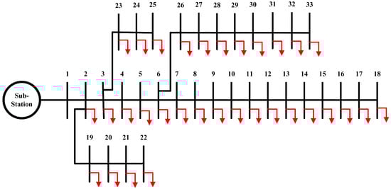
Figure 9.
Single line diagram of IEEE 33-bus system.
4.1.1. TEES Performance Evaluation
This research paper considers some assumptions in order to address the ODGA problem. The DGs’ uncertainty is not taken into account. And the annual energy loss is calculated using a constant power load model. Technical, cost-economic, environmental, and social performance evaluations are evaluated across unity, 0.90, and 0.85 lagging power factors. The detailed results are presented in Table 5, Table 6 and Table 7.
Table 5.
TEES performance evaluations in S1/C1-3 for IEEE 33-bus ADN.
Table 6.
TEES performance evaluations in S2/C1-3 for IEEE 33-bus ADN.
Table 7.
TEES performance evaluations in S3/C1-3 for IEEE 33-bus ADN.
From a TPE aspect, S1/C3, S2/C3, and S3/C3 have the lowest PLoss and QLoss. On the other hand, achieves the best PLM and QLM. According to Figure 10, It is obvious that as DGPP increases, PLM and QLM increase as well. And voltage profile improves gradually. According to CEPE perspective, S1/C3, S2/C3, S3/C3 are observed to have the lowest CELoss. With increasing the penetrations of DGs from one to three in all scenarios, S1/C3, S2/C3, and S3/C3 are observed to have the greatest SELoss values when compared to other solutions as illustrated in Figure 11. CPDG, CQDG, and CAI values are also calculated for revenue and net profit comparison. As DGs penetration increases, revenue and net profit also increase. So, we can say that DGs integration have a positive impact on net profit. A comparative study of TC, Revenue, and Net profit in different scenarios is shown in Figure 12. From an EPE perspective, S1/C3, S2/C3, and S3/C3 have the lowest PE and WC. With the increasing penetration of DGs, PEM and WCM also increase as shown in Figure 13. Similarly, in SPE, it achieves the best LQ and SA results after the integration of DGs as depicted in Figure 14.
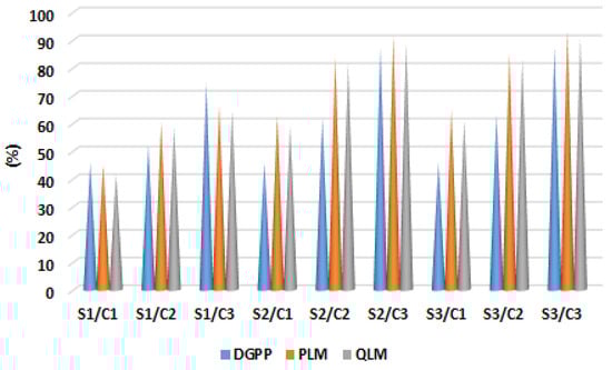
Figure 10.
Comparative study of PLM, QLM with DGPP in IEEE 33-bus system.
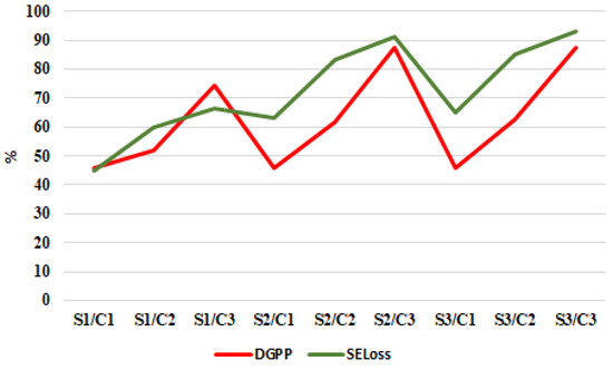
Figure 11.
Comparative study of SELoss with DGPP in IEEE 33-bus system.
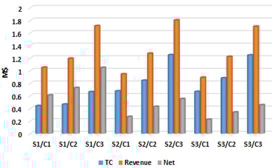
Figure 12.
Comparative study of TC, Revenue and Net profit in IEEE-33 bus system.
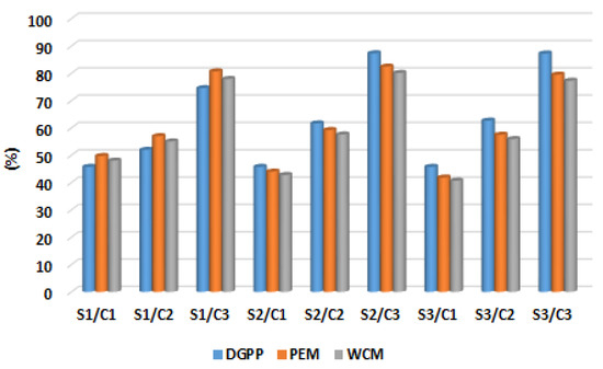
Figure 13.
Comparative study of PEM, WCM with DGPP in IEEE 33-bus system.
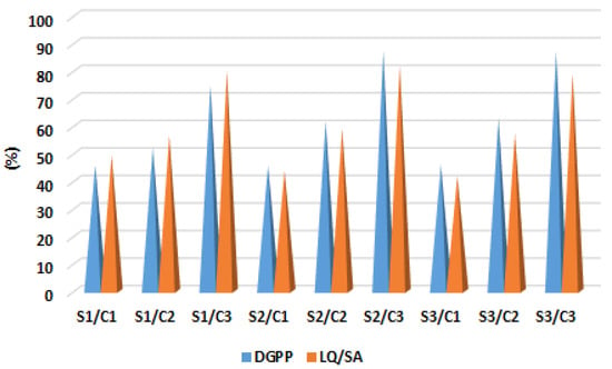
Figure 14.
Impact of LQ/SA wrt DGPP in IEEE-33 bus system.
Detailed evaluations of S1, S2, and S3 in terms of MCDM techniques are done. On the basis of evaluations across TEES, MCDM approaches are applied to get the trade-off. Alternatives S1/C3, S2/C3, and S3/C3 stands out from the other alternatives as shown in Figure 15, Figure 16 and Figure 17.
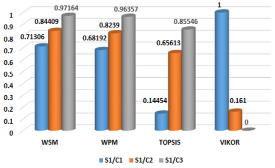
Figure 15.
TEES evaluation for scenario 1 at UPF in IEEE 33-bus system.
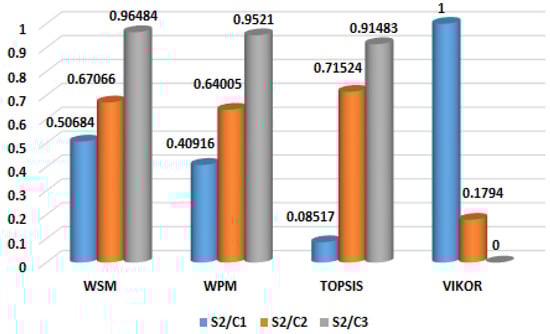
Figure 16.
TEES evaluation for scenario 2 at 0.90 LPF in IEEE 33-bus system.
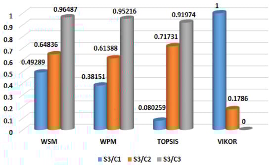
Figure 17.
TEES evaluation for scenario 2 at 0.85 LPF in IEEE 33-bus system.
4.1.2. Scenario 1
It has been found that ADN without DG results in more losses. Besides the type, the suboptimal DG capacity can result in increased system losses in a DN. In scenario 1, the proposed technique is used to optimize the locations and sizes of single and multiple DGs in order to reduce power losses. The results of simulations for various DG operating cases are presented and comparative analysis is done with other optimization methods at UPF as shown in Table 5 and Table 8 respectively. As shown by Table 8, the optimal locations of three DGs in S1/C3 using the proposed technique are 30, 24, and 14 with active power capacities of 1217 kW, 1175 kW, and 867 kW, respectively, resulting in a reduction of power losses from 210.1 kW to 70.6 kW, with a loss reduction (PLM) of 66.37%. The proposed method has the least power losses when compared to other optimization methods. This result is better than that from TLBO [49], QOTLBO [49], KHA [50], SIMBO-Q [51], QOSIMBO-Q [51], QOCSOS [52], IRRO [33], and MRFO [34]. Furthermore, the proposed method significantly improves all objective functions, including PLoss, Vmin, and VSI. Vmin gradually improves as the number of DGs integrated increases. Vmin increases from its base value 0.9042 (p.u) to 0.9790 (p.u) and VSI value is further improved to 0.8943 (p.u) from base value of 0.6672 (p.u) in S1/C3. Energy loss cost and energy loss savings are taken as comparative parameters in economic aspects. The proposed technique gives preferable results in terms of and as comes out o be 0.037128 M$ from proposed and MPA methods which are better than other techniques in Table 8.
Table 8.
Comparative results of DGs allocation for 33-bus network at UPF.
4.1.3. Scenario 2
In this scenario, the proposed technique is used to optimize the locations and sizes of single and multiple DGs in order to reduce active and reactive power losses at a fixed 0.90 LPF. The results of simulations for various DG operating cases C1-3 are presented in Table 6. As number of DG increases, reduces by 62.89%, 83.43%, and 91.38% in C1-3 respectively. Similarly are reduced by 58.85%, 81.28%, and 88.77%. The voltage profile is significantly improved to 0.9942 (p.u) and energy loss savings comes out to be 0.100891 M$ in case of three DGs.
4.1.4. Scenario 3
The proposed technique is used to optimize the locations and capacities of single and multiple DGs in order to minimize the power losses at 0.85 LPF. The results of simulations for various DG operating cases are presented and comparative analysis is done with other optimization methods as shown in Table 7 and Table 9 respectively. As shown by Table 9, the optimal locations of three DGs in S3/C3 using the proposed technique are 30, 24, and 13 with power ratings of 1570 kVA, 1310 kVA, and 932 kVA, respectively, resulting in a reduction of power losses from 210.1 kW to 14.4 kVA, with a loss minimization (PLM) of 93.14%. The proposed method has the minimum power losses when compared to other optimization methods. This result is better than that from MOTA [53], IMOEHO [54], MOPSO [55], MOCSOS [55], and I-DBEA [56]. Reactive power losses is also reduced from 142.4 kVAR (S0/C0_1) to 13.4 kVAR with a loss minimization (QLM) of 90.60% in S3/C3. Voltage profile and voltage stability are significantly improved to 0.9942 (p.u) and 0.9747 (p.u) respectively, as compared to other methods which are reported in Table 9. Energy loss savings comes out to be 0.102836 M$ from both proposed and MPA techniques which are more than reported methods in MOTA [53], IMOEHO [54], MOPSO [55], MOCSOS [55], and I-DBEA [56].
Table 9.
Comparative results of DGs allocation for 33-bus network at 0.85 LPF.
4.1.5. Scenario 4
In this scenario, multiple DGs are optimally placed at optimal power factors. S4/C3_1 shows the results of three DGs, optimally placed at 0.70, 0.90, and 0.82 OPF as presented in Table 10. is reduced to 11.7 kW with a loss minimization of 94.41% which is comparatively equal to SFSA [57], SOS [52], and QOCSOS [52]. Table 11 shows that Vmin and VSI are significantly improved to 0.9942 (p.u) and 0.9801 (p.u) respectively, which are better than reported methods such as SFSA [57], SOS [52], and QOCSOS [52]. Energy loss cost comes out to be 0.006175 M$ from both proposed and MPA techniques which is better than the reported methods. Figure 18 shows the improvement in the voltage profiles of four different scenarios of DGs.
Table 10.
TEES performance evaluations in ADNs at OPF.
Table 11.
Comparative results of DGs allocation for 33-bus network at OPF.
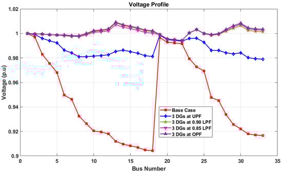
Figure 18.
Bus voltage profile of 33-bus network.
4.1.6. Performance Analysis for the Proposed Method
For the case studies in scenarios S1-3, the MFO outperforms the MPA in terms of convergence rate. The convergence characteristic of the proposed technique and MPA for case 3, which represents three DGs integration of Type I, is depicted in Figure 19. Similarly, the convergence characteristics of the proposed technique and MPA for S2/C3, which represents three DGs integration of Type III, are shown in Figure 20. In comparison to MPA, the proposed approach gets the minimum objective function in less iterations.
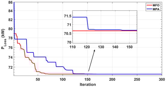
Figure 19.
Convergence curves of MFO and MPA for Scenario 1 of 33-bus network.
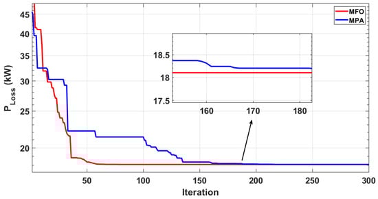
Figure 20.
Convergence curves of MFO and MPA for Scenario 2 of 33-bus network.
4.2. Test System 2
The benchmarking network IEEE 69-bus ADN, which is used to test and compare the various types of DG units is shown in Figure 21. This system consists of 69 buses and 68 branches. The total active power load (PLD) of this system is 3802.2 kW and the reactive power load (QLD) is 2694.6 kVAR, at the base values of 100 MVA and 12.66 kV. In base case S0/C0_2, total active power loss (PLoss) of 224.6 kW and reactive power loss (QLoss) of 101.9 kVAR. And minimum voltage magnitude (Vmin) of the system is 0.9102 (p.u) at bus 18.
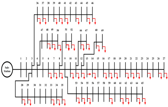
Figure 21.
Single line diagram of IEEE 69-bus system.
4.2.1. TEES Performance Evaluation
TEES performance evaluations are evaluated across unity, 0.90, and 0.85 lagging power factors in the 69-bus system. The detailed results are presented in Table 12, Table 13 and Table 14. From a TPE aspect, S1/C3, S2/C3, and S3/C3 have the lowest and . On the other hand, achieves the best and . According to Figure 22 It is clear that as DGPP increases, PLM and QLM increase as well. And voltage profile improves gradually. According to CEPE perspective, S1/C3, S2/C3, S3/C3 are observed to have the lowest CELoss. With increasing the penetrations of DGs from one to three in all scenarios, S1/C3, S2/C3, and S3/C3 are observed to have the greatest SELoss values when compared to other solutions as depicted in Figure 23. CPDG, CQDG, and CAI values are also calculated for revenue and net profit comparison. As DGs penetration increases, revenue and net profit also increase. So, we can say that DGs integration have a positive impact on net profit. A comparative study of TC, Revenue, and Net profit in the IEEE 69-bus system is given in Figure 24. From an EPE perspective, S1/C3, S2/C3, and S3/C3 have the lowest PE and WC. With the increasing penetration of DGs, PEM and WCM also increase as shown in Figure 25. Similarly, in SPE, it achieves the best LQ and SA results after the integration of DGs as depicted in Figure 26.
Table 12.
TEES performance evaluations in S1/C1-3 for IEEE 69-bus ADN.
Table 13.
TEES performance evaluations in S2/C1-3 for IEEE 69-bus ADN.
Table 14.
TEES performance evaluations in S3/C1-3 for IEEE 69-bus ADN.
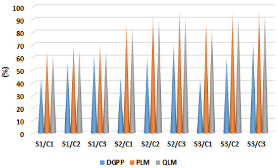
Figure 22.
Comparative study of PLM, QLM with DGPP in IEEE 69-bus system.
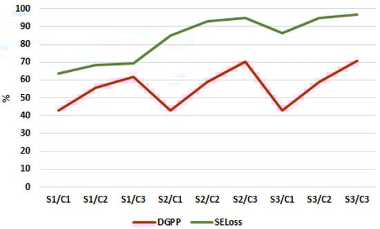
Figure 23.
Comparative study of SELoss with DGPP in IEEE 69-bus system.
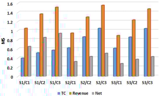
Figure 24.
Comparative study of TC, Revenue and Net profit in IEEE-69 bus system.
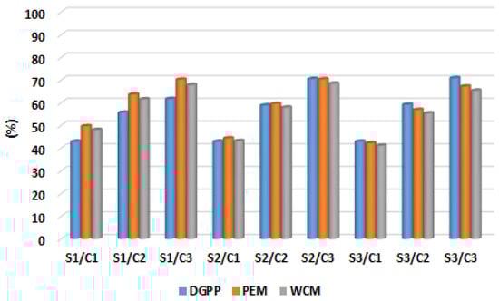
Figure 25.
Comparative study of PEM, WCM with DGPP in IEEE 69-bus system.
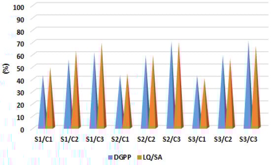
Figure 26.
Impact of LQ/SA wrt DGPP in IEEE-69 bus system.
Detailed evaluations of S1, S2, and S3 in terms of MCDM techniques are done in the IEEE 69-bus system. On the basis of evaluations across TEES, four different MCDM methods are applied to get the trade-off. Alternatives S1/C3, S2/C3, and S3/C3 stands out from the other alternatives as shown in Figure 27, Figure 28 and Figure 29.
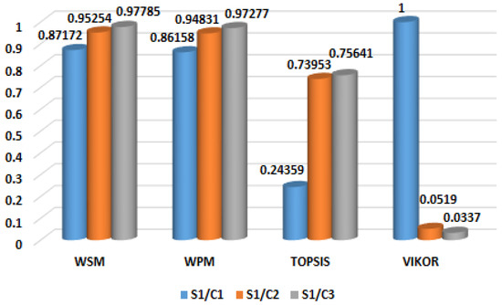
Figure 27.
TEES evaluation for scenario 1 at UPF in IEEE 69-bus system.
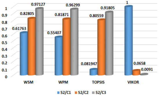
Figure 28.
TEES evaluation for scenario 2 at 0.90 LPF in IEEE 69-bus system.
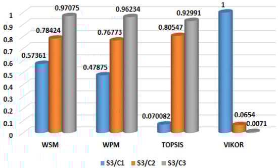
Figure 29.
TEES evaluation for scenario 3 at 0.85 LPF in IEEE 69-bus system.
4.2.2. Scenario 1
In this scenario of 69-bus, the proposed technique is used to optimize the locations and sizes of single and multiple DGs in order to minimize power losses. The results of simulations for various DG operating cases are presented and comparative analysis is done with other optimization techniques at UPF as shown in Table 12 and Table 15 respectively. As shown by Table 15, the optimal places of three DGs in S1/C3 using the proposed technique are found to be 61, 18, and 66 with power ratings of 2000 kVA, 451 kVA, and 425 kVA, respectively, resulting in a reduction of power losses from 224.6 kW to 68.9 kW, with a loss minimization (PLM) of 69.30%. The proposed method has the lowest power losses when compared to other optimization methods. This result is far better than that from TLBO [49], QOTLBO [49], KHA [50], SIMBO-Q [51], QOSIMBO-Q [51], QOCSOS [52], IRRO [33], and MRFO [34]. Furthermore, the proposed method significantly improves other objective functions, including PLoss, Vmin, and VSI. Vmin gradually improves as the number of DGs integrated increases. Vmin increases from its base value 0.9102 (p.u) to 0.9911 (p.u) and VSI is further improved to 0.9694 (p.u) from base value of 0.6832 (p.u) in S1/C3. In economic aspects, energy loss cost and energy loss savings are considered as comparative parameters. The proposed technique gives better results in terms of and as comes out o be 0.037128 M$ from proposed and MPA methods which are better than other techniques in Table 15.
Table 15.
Comparative results of DGs allocation for 69-bus network at UPF.
4.2.3. Scenario 2
The proposed technique is used to optimize the locations and sizes of single and multiple DGs in order to reduce active and reactive power losses at fixed 0.90 LPF. The results of simulations for various DG operating cases C1-3 are presented in Table 13. As number of DG increases, reduces by 84.91%, 93.16%, and 95.05% in C1-3 respectively. Similarly are reduced by 82.87%, 89.76%, and 91.01%. Voltage profile and VSI are significantly improved to 0.9943 (p.u) and 0.9949 (p.u) respectively in S2/C3. Energy loss saving has increased to 0.112213 M$ with the penetration of three DGs.
4.2.4. Scenario 3
The proposed technique is used to optimize the locations and capacities of single and multiple DGs in order to minimize the power losses at 0.85 LPF. The results of simulations for various DG operating cases are presented and comparative analysis is done with other optimization methods as shown in Table 14 and Table 16 respectively. As shown by Table 16, the optimal locations of three DGs in S3/C3 using the proposed technique are 61, 11, and 18 with power ratings of 2000 kVA, 798 kVA, and 504 kVA, respectively, resulting in a minimization of power losses from 224.6 kW to 7.0 kW, with a loss minimization (PLM) of 96.86%. The proposed method has the minimum power losses when compared to other optimization methods. This result is better than that from PSO [58], IMOHS [59], and I-DBEA [56]. Reactive power losses is also reduced from 101.9914 kVAR (S0/C0_2) to 7.27 kVAR with a loss minimization (QLM) of 92.86% in S3/C3. Voltage profile and voltage stability are significantly improved to 0.9943 (p.u) and 0.9944 (p.u) respectively, as compared to other methods which are reported in Table 14. Energy loss saving comes out to be 0.114353 M$ from both proposed and MPA techniques which are more than reported methods in PSO [58], IMOHS [59], and I-DBEA [56].
Table 16.
Comparative results of DGs allocation for 69-bus network at 0.85 LPF.
4.2.5. Scenario 4
Multiple DGs are optimally placed at optimal power factors in the 69-bus system. S4/C3_2 shows the results of three DGs, optimally placed at 0.80, 0.82, and 0.82 OPF as presented in Table 10. is reduced to 6.4 kW with a loss minimization of 97.14% which is comparatively better than HHO [37] as illustrated in Table 17. Vmin and VSI are significantly improved to 0.9943 (p.u) and 0.9934 (p.u) respectively, which are better than reported methods such as HHO [37], and QOCSOS [52]. Energy loss cost comes out to be 0.003379 M$ from both proposed and MPA techniques which is better than the reported methods. Figure 30 shows the improvement in the voltage profiles of four different scenarios of DGs operating cases.
Table 17.
Comparative results of DGs allocation for 69-bus network at OPF.
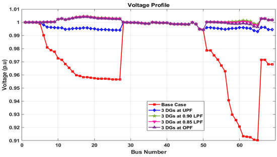
Figure 30.
Bus voltage profile of 69-bus network.
4.2.6. Performance Analysis for the Proposed Method
For the case studies in scenario S1-3, the MFO performs much better than the MPA algorithm in terms of convergence. The convergence characteristic of the proposed technique and MPA for S1/C3, which represents three DGs integration of Type I, is depicted in Figure 31. Similarly, the convergence characteristics of the proposed technique and MPA for S2/C3, which represents three DGs integration of Type III, are shown in Figure 32. In comparison to MPA, the suggested approach takes less iterations to achieve the minimum objective function.
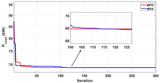
Figure 31.
Convergence curves of MFO and MPA for Scenario 1 of 69-bus network.
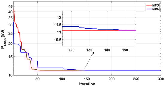
Figure 32.
Convergence curves of MFO and MPA for Scenario 2 of 69-bus network.
5. Conclusions
In this paper, energy planning is evaluated broadly on technical, cost-economic, environmental, and social indices using the MCSP approach based on nature-inspired optimization techniques. The proposed MFO and MPA have been effectively implemented for resolving the ODGA problem in ADNs with multiple criteria. Two benchmark test systems were used to evaluate MFO’s effectiveness and superiority over MPA. The results showed that MFO has a better and faster convergence rate than MPA, as well as MFO’s supremacy in attaining the best DG allocation in the ADNs. MCDM methods such as WSM, WPM, TOPSIS, and VIKOR have been used in taking decisions and selecting the best solution among several alternatives for conflicting criteria. The appropriate weighting factors for different criteria have been decided by the analytic hierarchy process. The results from TEES evaluations demonstrate greater improvements in annual energy loss reduction and cost savings as compared with those of the previous methods reported in the literature. According to studies, DGs have substantial potential for improving the distribution system’s performance. Furthermore, the results obtained revealed that the highest loss reduction in the 33-bus and 69-bus systems were 94.41% and 97.14%, and the maximum VSI was 0.9801 (p.u) and 0.9934 (p.u), respectively; however, the minimum Vmin for the given test systems were 0.9942 (p.u) and 0.9943 (p.u). A significant reduction in PE and WC was also observed in this study.
The appropriate allocation of DGs considering different levels of DG penetration at varying loads should be investigated in future work. Furthermore, the uncertainty modeling of renewable-based DGs would also be considered.
Author Contributions
Conceptualization, S.A.A.K., A.A. and Z.A.K.; methodology, S.A.A.K., Z.A.K., A.A. and D.R.S.; software, M.W.K.; validation, M.W.K., S.A.A.K. and Z.A.K.; formal analysis, M.W.K., A.A. an D.R.S.; investigation, M.W.K.; resources, Z.A.K. and A.A.; data curation, M.W.K. and A.A.; writing—original draft preparation, M.W.K. and S.A.A.K.; writing—review and editing, Z.A.K., A.A. and D.R.S.; visualization, M.W.K.; supervision, S.A.A.K. and Z.A.K.; project administration, S.A.A.K., Z.A.K. and A.A.; funding acquisition, A.A. All authors have read and agreed to the published version of the manuscript.
Funding
The main author extends his appreciation to the Deputyship for Research & Innovation, Ministry of Education in Saudi Arabia for funding this research work through project number (IFP-2020-99).
Institutional Review Board Statement
Not applicable.
Informed Consent Statement
Not applicable.
Data Availability Statement
Not applicable.
Acknowledgments
The main author extends his appreciation to the Deputyship for Research & Innovation, Ministry of Education in Saudi Arabia for funding this research work through project number (IFP-2020-99).
Conflicts of Interest
The authors declare no conflict of interest.
Abbreviations
The following abbreviations are used in this paper:
| ADN | Active distribution network |
| AF | Annualized factor |
| CE | Cost of electricity unit |
| CAI | Cost of annual investment |
| CPDG | Cost of active power DG |
| CQDG | Cost of reactive power DG |
| CUDG | Cost of a DG unit |
| CEPI | Cost-economic performance indices |
| Cost of energy loss/active power loss cost | |
| DG | Distributed generation |
| DN | Distribution network |
| EPI | Environmental performance indices |
| EgAj | Amount of energy produced by jth conventional power plant without employment of DG |
| Egj | Amount of energy produced by jth conventional power plant with employment of DG |
| Amount of energy produced by kth DG plant | |
| EFi | Emission factor of ith pollutant |
| IR | Interest rate based on annual cost |
| LUI | Land use intensity |
| LPF | Lagging power factor |
| M$ | Millions of USD |
| MCDM | Multiple-criteria decision making |
| ODGA | Optimal DG allocation |
| OPF | Optimal power factor |
| PF | Power factor |
| PEM | Pollution emission minimization |
| PLD | Active power load |
| PLoss | Active power loss |
| PLM | Active power loss minimization |
| PSS | Active power release from sub-station |
| QLD | Reactive power load |
| QLoss | Reactive power loss |
| QLM | Reactive power loss minimization |
| QSS | Reactive power release from sub-station |
| SPI | Social performance indices |
| Energy loss saving | |
| TEES | Techno-economic-environmental-social |
| TPI | Technical performance indices |
| UPF | Unity power factor |
| WCF | Water consumption factor |
| WCM | Water consumption minimization |
References
- Haseeb, M.; Kazmi, S.A.A.; Malik, M.M.; Ali, S.; Bukhari, S.B.A.; Shin, D.R. Multi objective based framework for energy management of smart micro-grid. IEEE Access 2020, 8, 220302–220319. [Google Scholar] [CrossRef]
- Wagh, M.; Kulkarni, V. Modeling and optimization of integration of Renewable Energy Resources (RER) for minimum energy cost, minimum CO2 Emissions and sustainable development, in recent years: A review. Mater. Today Proc. 2018, 5, 11–21. [Google Scholar] [CrossRef]
- Ackermann, T.; Andersson, G.; Söder, L. Distributed generation: A definition. Electr. Power Syst. Res. 2001, 57, 195–204. [Google Scholar] [CrossRef]
- Selim, A.; Kamel, S.; Jurado, F. Efficient optimization technique for multiple DG allocation in distribution networks. Appl. Soft Comput. 2020, 86, 105938. [Google Scholar] [CrossRef]
- Quadri, I.A.; Bhowmick, S.; Joshi, D. A hybrid teaching–learning-based optimization technique for optimal DG sizing and placement in radial distribution systems. Soft Comput. 2019, 23, 9899–9917. [Google Scholar] [CrossRef]
- Suresh, M.; Belwin, E.J. Optimal DG placement for benefit maximization in distribution networks by using Dragonfly algorithm. Renew. Wind. Water Sol. 2018, 5, 1–8. [Google Scholar] [CrossRef]
- Khodabakhshian, A.; Andishgar, M.H. Simultaneous placement and sizing of DGs and shunt capacitors in distribution systems by using IMDE algorithm. Int. J. Electr. Power Energy Syst. 2016, 82, 599–607. [Google Scholar] [CrossRef]
- Selim, A.; Kamel, S.; Mohamed, A.A.; Elattar, E.E. Optimal Allocation of Multiple Types of Distributed Generations in Radial Distribution Systems Using a Hybrid Technique. Sustainability 2021, 13, 6644. [Google Scholar] [CrossRef]
- Hung, D.Q.; Mithulananthan, N.; Bansal, R. Analytical expressions for DG allocation in primary distribution networks. IEEE Trans. Energy Convers. 2010, 25, 814–820. [Google Scholar] [CrossRef]
- Georgilakis, P.S.; Hatziargyriou, N.D. Optimal distributed generation placement in power distribution networks: Models, methods, and future research. IEEE Trans. Power Syst. 2013, 28, 3420–3428. [Google Scholar] [CrossRef]
- Jain, S.; Kalambe, S.; Agnihotri, G.; Mishra, A. Distributed generation deployment: State-of-the-art of distribution system planning in sustainable era. Renew. Sustain. Energy Rev. 2017, 77, 363–385. [Google Scholar] [CrossRef]
- Trivedi, I.N.; Jangir, P.; Bhoye, M.; Jangir, N. An economic load dispatch and multiple environmental dispatch problem solution with microgrids using interior search algorithm. Neural Comput. Appl. 2018, 30, 2173–2189. [Google Scholar] [CrossRef]
- Marwali, M.N.; Jung, J.W.; Keyhani, A. Stability analysis of load sharing control for distributed generation systems. IEEE Trans. Energy Convers. 2007, 22, 737–745. [Google Scholar] [CrossRef]
- Esmaili, M.; Firozjaee, E.C.; Shayanfar, H.A. Optimal placement of distributed generations considering voltage stability and power losses with observing voltage-related constraints. Appl. Energy 2014, 113, 1252–1260. [Google Scholar] [CrossRef]
- Parhizi, S.; Lotfi, H.; Khodaei, A.; Bahramirad, S. State of the art in research on microgrids: A review. IEEE Access 2015, 3, 890–925. [Google Scholar] [CrossRef]
- Naik, S.G.; Khatod, D.; Sharma, M. Optimal allocation of combined DG and capacitor for real power loss minimization in distribution networks. Int. J. Electr. Power Energy Syst. 2013, 53, 967–973. [Google Scholar] [CrossRef]
- Mahmoud, K.; Yorino, N.; Ahmed, A. Optimal distributed generation allocation in distribution systems for loss minimization. IEEE Trans. Power Syst. 2015, 31, 960–969. [Google Scholar] [CrossRef]
- Ehsan, A.; Yang, Q. Optimal integration and planning of renewable distributed generation in the power distribution networks: A review of analytical techniques. Appl. Energy 2018, 210, 44–59. [Google Scholar] [CrossRef]
- Niknam, T.; Taheri, S.I.; Aghaei, J.; Tabatabaei, S.; Nayeripour, M. A modified honey bee mating optimization algorithm for multiobjective placement of renewable energy resources. Appl. Energy 2011, 88, 4817–4830. [Google Scholar] [CrossRef]
- Moradi, M.H.; Abedini, M. A combination of genetic algorithm and particle swarm optimization for optimal DG location and sizing in distribution systems. Int. J. Electr. Power Energy Syst. 2012, 34, 66–74. [Google Scholar] [CrossRef]
- García, J.A.M.; Mena, A.J.G. Optimal distributed generation location and size using a modified teaching–learning based optimization algorithm. Int. J. Electr. Power Energy Syst. 2013, 50, 65–75. [Google Scholar] [CrossRef]
- Ameli, A.; Bahrami, S.; Khazaeli, F.; Haghifam, M.R. A multiobjective particle swarm optimization for sizing and placement of DGs from DG owner’s and distribution company’s viewpoints. IEEE Trans. Power Deliv. 2014, 29, 1831–1840. [Google Scholar] [CrossRef]
- Sheng, W.; Liu, K.y.; Liu, Y.; Ye, X.; He, K. Reactive power coordinated optimisation method with renewable distributed generation based on improved harmony search. IET Gener. Transm. Distrib. 2016, 10, 3152–3162. [Google Scholar] [CrossRef]
- Ali, E.; Abd Elazim, S.; Abdelaziz, A. Ant Lion Optimization Algorithm for optimal location and sizing of renewable distributed generations. Renew. Energy 2017, 101, 1311–1324. [Google Scholar] [CrossRef]
- Abou El-Ela, A.A.; El-Sehiemy, R.A.; Abbas, A.S. Optimal placement and sizing of distributed generation and capacitor banks in distribution systems using water cycle algorithm. IEEE Syst. J. 2018, 12, 3629–3636. [Google Scholar] [CrossRef]
- Ramadan, A.; Ebeed, M.; Kamel, S.; Nasrat, L. Optimal allocation of renewable energy resources considering uncertainty in load demand and generation. In Proceedings of the 2019 IEEE Conference on Power Electronics and Renewable Energy (CPERE); 2019; pp. 124–128. [Google Scholar]
- Mohamed, M.A.E.S.; Mohammed, A.A.E.; Abd Elhamed, A.M.; Hessean, M.E. Optimal allocation of photovoltaic based and DSTATCOM in a distribution network under multi load levels. Eur. J. Eng. Technol. Res. 2019, 4, 114–119. [Google Scholar]
- Sambaiah, K.S.; Jayabarathi, T. Optimal allocation of renewable distributed generation and capacitor banks in distribution systems using salp swarm algorithm. Int. J. Renew. Energy Res. 2019, 9, 96–107. [Google Scholar]
- Remha, S.; Chettih, S.; Arif, S. A novel multi-objective bat algorithm for optimal placement and sizing of distributed generation in radial distributed systems. Adv. Electr. Electron. Eng. 2018, 15, 736–746. [Google Scholar] [CrossRef]
- Ganguly, S.; Samajpati, D. Distributed generation allocation with on-load tap changer on radial distribution networks using adaptive genetic algorithm. Appl. Soft Comput. 2017, 59, 45–67. [Google Scholar] [CrossRef]
- Prasad, C.H.; Subbaramaiah, K.; Sujatha, P. Cost–benefit analysis for optimal DG placement in distribution systems by using elephant herding optimization algorithm. Renew. Wind Water Solar 2019, 6, 1–12. [Google Scholar] [CrossRef]
- Almabsout, E.A.; El-Sehiemy, R.A.; An, O.N.U.; Bayat, O. A hybrid local search-genetic algorithm for simultaneous placement of DG units and shunt capacitors in radial distribution systems. IEEE Access 2020, 8, 54465–54481. [Google Scholar] [CrossRef]
- Nagaballi, S.; Kale, V.S. Pareto optimality and game theory approach for optimal deployment of DG in radial distribution system to improve techno-economic benefits. Appl. Soft Comput. 2020, 92, 106234. [Google Scholar] [CrossRef]
- Hemeida, M.G.; Ibrahim, A.A.; Mohamed, A.A.A.; Alkhalaf, S.; El-Dine, A.M.B. Optimal allocation of distributed generators DG based Manta Ray Foraging Optimization algorithm (MRFO). Ain Shams Eng. J. 2021, 12, 609–619. [Google Scholar] [CrossRef]
- Rupa, J.M.; Ganesh, S. Power flow analysis for radial distribution system using backward/forward sweep method. Int. J. Electr. Comput. Electron. Commun. Eng. 2014, 8, 1540–1544. [Google Scholar]
- Buayai, K.; Ongsakul, W.; Mithulananthan, N. Multi-objective micro-grid planning by NSGA-II in primary distribution system. Eur. Trans. Electr. Power 2012, 22, 170–187. [Google Scholar] [CrossRef]
- Selim, A.; Kamel, S.; Alghamdi, A.S.; Jurado, F. Optimal placement of DGs in distribution system using an improved harris hawks optimizer based on single-and multi-objective approaches. IEEE Access 2020, 8, 52815–52829. [Google Scholar] [CrossRef]
- Murty, V.V.; Kumar, A. Optimal placement of DG in radial distribution systems based on new voltage stability index under load growth. Int. J. Electr. Power Energy Syst. 2015, 69, 246–256. [Google Scholar] [CrossRef]
- Kazmi, S.A.A.; Ameer Khan, U.; Ahmad, W.; Hassan, M.; Ibupoto, F.A.; Bukhari, S.B.A.; Ali, S.; Malik, M.M.; Shin, D.R. Multiple (TEES)-Criteria-Based Sustainable Planning Approach for Mesh-Configured Distribution Mechanisms across Multiple Load Growth Horizons. Energies 2021, 14, 3128. [Google Scholar] [CrossRef]
- Oda, E.S.; Abd El Hamed, A.M.; Ali, A.; Elbaset, A.A.; Abd El Sattar, M.; Ebeed, M. Stochastic Optimal Planning of Distribution System Considering Integrated Photovoltaic-Based DG and DSTATCOM Under Uncertainties of Loads and Solar Irradiance. IEEE Access 2021, 9, 26541–26555. [Google Scholar] [CrossRef]
- Chiradeja, P.; Ramakumar, R. An approach to quantify the technical benefits of distributed generation. IEEE Trans. Energy Convers. 2004, 19, 764–773. [Google Scholar] [CrossRef]
- Baldwin, S. Carbon footprint of electricity generation. Lond. Parliam. Off. Sci. Technol. 2006, 268. [Google Scholar]
- Macknick, J.; Newmark, R.; Heath, G.; Hallett, K. Review of Operational Water Consumption and Withdrawal Factors for Electricity Generating Technologies; Technical Report; National Renewable Energy Lab.(NREL): Golden, CO, USA, 2011. [Google Scholar]
- Fritsche, U.; Berndes, G.; Cowie, A.; Johnson, F.; Dale, V.; Langeveld, H.; Sharma, N.; Watson, H.; Woods, J. Energy and Land Use: Global Land Outlook Working Paper; United Nations Convention to Combat Desertification (UNCCD): Bonn, Germany, 2017. [Google Scholar]
- Kumar, A.; Sah, B.; Singh, A.R.; Deng, Y.; He, X.; Kumar, P.; Bansal, R. A review of multi criteria decision making (MCDM) towards sustainable renewable energy development. Renew. Sustain. Energy Rev. 2017, 69, 596–609. [Google Scholar] [CrossRef]
- Jin, J.; Rothrock, L.; McDermott, P.L.; Barnes, M. Using the analytic hierarchy process to examine judgment consistency in a complex multiattribute task. IEEE Trans. Syst. Man, Cybern. Part A Syst. Hum. 2010, 40, 1105–1115. [Google Scholar] [CrossRef]
- Mirjalili, S. Moth-flame optimization algorithm: A novel nature-inspired heuristic paradigm. Knowl.-Based Syst. 2015, 89, 228–249. [Google Scholar] [CrossRef]
- Faramarzi, A.; Heidarinejad, M.; Mirjalili, S.; Gandomi, A.H. Marine Predators Algorithm: A nature-inspired metaheuristic. Expert Syst. Appl. 2020, 152, 113377. [Google Scholar] [CrossRef]
- Sultana, S.; Roy, P.K. Multi-objective quasi-oppositional teaching learning based optimization for optimal location of distributed generator in radial distribution systems. Int. J. Electr. Power Energy Syst. 2014, 63, 534–545. [Google Scholar] [CrossRef]
- Sultana, S.; Roy, P.K. Krill herd algorithm for optimal location of distributed generator in radial distribution system. Appl. Soft Comput. 2016, 40, 391–404. [Google Scholar] [CrossRef]
- Sharma, S.; Bhattacharjee, S.; Bhattacharya, A. Quasi-Oppositional Swine Influenza Model Based Optimization with Quarantine for optimal allocation of DG in radial distribution network. Int. J. Electr. Power Energy Syst. 2016, 74, 348–373. [Google Scholar] [CrossRef]
- Truong, K.H.; Nallagownden, P.; Elamvazuthi, I.; Vo, D.N. A quasi-oppositional-chaotic symbiotic organisms search algorithm for optimal allocation of DG in radial distribution networks. Appl. Soft Comput. 2020, 88, 106067. [Google Scholar] [CrossRef]
- Meena, N.K.; Swarnkar, A.; Gupta, N.; Niazi, K.R. Multi-objective Taguchi approach for optimal DG integration in distribution systems. IET Gener. Transm. Distrib. 2017, 11, 2418–2428. [Google Scholar] [CrossRef]
- Meena, N.K.; Parashar, S.; Swarnkar, A.; Gupta, N.; Niazi, K.R. Improved elephant herding optimization for multiobjective DER accommodation in distribution systems. IEEE Trans. Ind. Inform. 2017, 14, 1029–1039. [Google Scholar] [CrossRef]
- Saha, S.; Mukherjee, V. A novel multiobjective chaotic symbiotic organisms search algorithm to solve optimal DG allocation problem in radial distribution system. Int. Trans. Electr. Energy Syst. 2019, 29, e2839. [Google Scholar] [CrossRef]
- Ali, A.; Keerio, M.; Laghari, J. Optimal Site and Size of Distributed Generation Allocation in Radial Distribution Network Using Multi-objective Optimization. J. Mod. Power Syst. Clean Energy 2020, 9, 404–415. [Google Scholar] [CrossRef]
- Nguyen, T.P.; Vo, D.N. A novel stochastic fractal search algorithm for optimal allocation of distributed generators in radial distribution systems. Appl. Soft Comput. 2018, 70, 773–796. [Google Scholar] [CrossRef]
- AlRashidi, M.; AlHajri, M. Optimal planning of multiple distributed generation sources in distribution networks: A new approach. Energy Convers. Manag. 2011, 52, 3301–3308. [Google Scholar] [CrossRef]
- Nekooei, K.; Farsangi, M.M.; Nezamabadi-Pour, H.; Lee, K.Y. An improved multi-objective harmony search for optimal placement of DGs in distribution systems. IEEE Trans. Smart Grid 2013, 4, 557–567. [Google Scholar] [CrossRef]


Disclaimer/Publisher’s Note: The statements, opinions and data contained in all publications are solely those of the individual author(s) and contributor(s) and not of MDPI and/or the editor(s). MDPI and/or the editor(s) disclaim responsibility for any injury to people or property resulting from any ideas, methods, instructions or products referred to in the content. |
© 2022 by the authors. Licensee MDPI, Basel, Switzerland. This article is an open access article distributed under the terms and conditions of the Creative Commons Attribution (CC BY) license (https://creativecommons.org/licenses/by/4.0/).