Article

The Coupled Thermal-Structural Resonance Reliability Sensitivity Analysis of Gear-Rotor System with Random Parameters

1
School of Mechanical and Power Engineering, Yingkou Institute of Technology, Yingkou 115014, China
2
School of Mechanical Engineering and Automation, Northeastern University, Shenyang 110819, China
*
Author to whom correspondence should be addressed.
Sustainability 2023, 15(1), 255; https://doi.org/10.3390/su15010255
Submission received: 31 October 2022 / Revised: 9 December 2022 / Accepted: 16 December 2022 / Published: 23 December 2022
(This article belongs to the Special Issue Reliability and Optimization for Engineering Design)

Abstract

:
The resonance of the gear-rotor system will produce a large number of responses that do not exceed the threshold value, resulting in structural fatigue failure and transmission failure, affecting its life and reliability. It is particularly critical to consider the temperature rise under high-speed and heavy-load conditions. Therefore, the research will take the main drive gear-rotor system of a certain type of aeroengine accessory gearbox as the research object, consider the influence of the temperature field on the natural frequency of the gear-rotor system, and take the difference between the natural frequency of the gear-rotor system and the excitation frequency (gear meshing frequency) as the performance function. The PC-Kriging and adaptive design of experimental strategies are applied to the thermal-structural coupling parametric model to analyze the resonance reliability and sensitivity of the gear-rotor system. For complex mechanical mechanisms, the method has better accuracy than other surrogate models and greatly saves the time of finite element simulation in reliability analysis. The results show that the natural frequency of a gear rotor decreases with an increase in temperature, and the natural frequency of different orders varies with the change in temperature. The influence of the sensitivity of different random parameters on the resonance reliability of the gear-rotor system is obtained. Reliability research on resonance failure of high-speed and heavy-load aviation gear-rotor systems considering random parameters under a temperature rise field has important practical engineering application value and scientific research significance.

1. Introduction

As a key component of mechanical transmission system, gear-rotor system has been widely applied in aerospace, automotive, marine, engineering machinery and other fields. In engineering practice, the gear-rotor system is inevitably disturbed by various random factors, such as the structural dimensions of each gear are different even in a batch of manufactured gears due to environmental, measurement and human factors during machining and assembly. In addition, random factors such as damping and external excitation exist in the transmission process, resulting in different vibration parameters such as natural frequency and amplitude of each gear-rotor system. The excitation frequency inevitably falls within the range of natural frequency, thus causing the resonance of the gear-rotor system, and the change of the temperature rise of the gear rotor will cause the change of the mechanical properties of the material, and then cause the change of the natural frequency, and also lead to the resonance of the gear-rotor system. In the transmission of high speed and heavy load gear rotor system, more heat will be generated, leading to thermal deformation of gear and non-involute error, resulting in increased vibration, noise, accelerated wear, and shortened gear life [1]. Therefore, it is of practical significance to study the resonance reliability sensitivity analysis of gear-rotor system with random parameters considering temperature rise.
At present, the reliability sensitivity analysis of gear-rotor system for uncertain factors is seldom studied [2,3], and the resonance reliability sensitivity analysis of gear-rotor system considering thermal factors is even less. In the practical engineering application of reliability analysis, because its performance function is usually complex, strongly non-linear, or implicit, it cannot be expressed by display, so it needs to apply the finite element simulation analysis. When the mechanical structure is highly nonlinear or complex, the time of a single analysis is usually very time-consuming (hours or days), and a large number of finite element analysis operations (tens or hundreds or more) are required to obtain satisfactory results, which is not acceptable in engineering practice. Therefore, the surrogate model technologies such as support vector machine [4], artificial neural network [5,6], response surface method [7,8] and Kriging model have been widely used and developed to solve similar problems [9,10,11,12,13] in recent years. In particular, the recently proposed surrogate model method [14,15,16] has been applied to the reliability analysis of aviation gear rotors, which provides great inspiration for this research. The Kriging model is the most widely applied in engineering, but it also has its own shortcomings. It can be seen that the accuracy of Kriging model with different basis functions is different [17]. If there are enough DoE points, the influence of the order of the basis function can be neglected. In reliability analysis, if the function is implicit and the number of SDoE points is small, the higher the order of the basis function, the more accurate the model is. However, with the increase in the size of X and the order of polynomial, the number of terms of basis function increases dramatically, which makes it difficult to calculate Kriging model in high-order reliability analysis (such as cube). Subsequently, Schobi [18] et al. proposed a new model method combining PCE and Kriging, named polynomial chaos -Kriging (PC-Kriging). Compared with the traditional Kriging model, PC-Kriging model has more advantages in the calculation of strong nonlinear and complex problems. Due to the relatively little further research on the model, especially in engineering applications. Therefore, the research will adopt the method of combining PC-Kriging model and adaptive design of experimental strategies to carry out the engineering application analysis of reliability sensitivity of aviation gear rotor system.
In this research, sensitivity analysis can determine the importance of random parameters and identify the random parameters that have the greatest influence on gear-rotor system and determine the sensitive and non-sensitive parameters of gear rotor system reliability under the influence of thermal factors, which has practical significance for guiding engineering application research. More importantly, the reliability and sensitivity analysis of the main transmission gear rotor system (complex engineering structure) of aviation accessory gearbox with PC-Kriging surrogate model is exploratory research, which can provide important reference value and theoretical basis for similar application research in engineering.

2. Thermal Theories and Numerical Simulation

The friction heat generated between the tooth surfaces mainly includes three aspects: sliding friction between the tooth surfaces, rolling friction and internal friction caused by metal elastic-plastic deformation. The proportion of internal friction caused by rolling friction, and metal-elastic-plastic deformation is very small, usually neglected, and only the heat generated by sliding friction is calculated [19].

2.1. Frictional Heat Generation

2.1.1. Average Contact Pressure

According to the Hertz formula, the maximum contact pressure of the meshing point p max is obtained:
p max = E F S 2 π R S b
where E = E 1 E 2 E 1 + E 2 is the comprehensive elastic modulus of the gear material; b is the tooth width; F S is normal load at the meshing point S and R S is comprehensive curvature radius.
The average contact pressure at the meshing point S is [20]:
p ¯ = π 4 p max

2.1.2. Relative Sliding Velocity

The speed of the driving gear and the driven gear at the normal meshing point S are the same, which ensures the continuous transmission of the gear. Figure 1 shows the transmission process of spur gear. The absolute speed v S 1 and v S 2 of the meshing point S along the tangent direction can be obtained, which can be expressed, respectively [21], as follows:
v S 1 = 2 π n 1 ( m z 1 2 sin α S ± d S ) 60 × 1000
v S 2 = 2 π n 2 ( m z 2 2 sin α S d S ) 60 × 1000
In Formulas (3) and (4), z 2 is the tooth number of the driven gear; n 1 is the rotation rate of the driving gear; n 2 is the rotation rate of the driven gear; d S is distance between the meshing point S and the point C on the meshing line.
The relative sliding speed of the driving and driven gear at the meshing point is
v = | v S 1 v S 2 |

2.1.3. The Average Heat Generation on Meshing Surface

Given tooth surface average friction coefficient f = 0.05 [21]. The frictional heat generation of the meshing surface is:
q = p ¯ f v
where p ¯ is average contact pressure in contact area (unit N); f is friction coefficient; v is the relative sliding velocity of the tooth (unit m/s).

2.2. Convection Heat Transfer Coefficient

2.2.1. Meshing Surface Heat Transfer Coefficient

The aerospace accessory gear-rotor system studied in the research has a high peripheral speed and is cooled by the oil-injection lubrication method. The lubricating oil is directly sprayed to the pitch position of the meshing surface, so that a large number of lubricants take away more heat. The meshing surface heat transfer coefficient h m is [22,23,24]:
h m = ω 2 π k o ρ o c o ( δ o r c v o H ) 1 4 q t o t
where ω is the angular velocity of the gear; k o is the thermal conductivity of the lubricating oil; ρ o is the density of the lubricating oil. c o is the specific heat capacity of the lubricating oil; δ o = k o / ρ o c o is the thermal conductivity of lubricating oil; v o is the kinematic viscosity of lubricating oil; r c is the pitch circle radius of the gear; H is the height of the tooth; q t o t is the standardized cooling quantity.

2.2.2. Convective Heat Transfer on Gear Flank

The flow patterns of oil-gas mixtures on the gear flank can be divided into three types: laminar flow, transition laminar flow and turbulent flow, which can be determined according to the range of Reynold number.
Laminar flow state: When R e mix 2 × 10 5 , the oil and gas mixture is laminar on the gear flank. Hartnett J P and Deland E C studies point out [25,26] that the convective heat transfer coefficient of laminar flow is independent of the rotational radius. Therefore, the convective heat transfer coefficient h D of the gear flank is:
h D = 0.308 k mix ( m D + 2 ) 0.5 P r mix 0.5 ( ω υ mix ) 0.5
Transition laminar flow state: When 2 × 10 5 < R e mix 2.5 × 10 5 , the oil and gas mixture is in a transitional laminar flow state on the gear flank, and the convective heat transfer coefficient h D on the gear flank is [27]:
h D = 10   × 10 20 k mix ( ω υ mix ) 4 r f 7
Turbulent state: When R e mix   >   2.5   ×   10 5 , the oil-gas mixture is in a turbulent state on the gear flank, the convective heat transfer coefficient h D is [28]:
h D = 0.0197 k mix ( m D + 2.6 ) 0.2 P r mix 0.6 ( ω υ mix ) 0.8 r f 0.6

2.2.3. Heat Transfer Coefficient of the Root Surface, the Top Surface and the Non-Meshing Surface

During the gear operation process, the top surface, the root surface and the non-meshing tooth surface are also forced to convective heat transfer with the oil and gas mixture, and the convective heat transfer coefficient h p can be approximated as 1/3–1/2 of the meshing surface [29].
h m 3 h p h m 2

2.2.4. Transmission Shaft Convection Heat Transfer Coefficient

(1) Heat transfer coefficient of external cylindrical surface
The convective heat transfer process between the external cylinder of the transmission shaft and the oil-gas mixture in the accessory casing can be simplified as the convective heat transfer problem of the horizontal rotating cylinder in the fluid [30,31]. Therefore, the convective heat transfer coefficient h g is
h g = 0.133 R e mix 2 3 P r mix 1 3 k mix d w
(2) Heat transfer coefficient of internal cylindrical surface
The convective heat transfer process of internal cylindrical surface can be equivalent to the convective heat transfer in a rotating cylinder with axial air flow [32]. The axial Reynolds number R e mix a and the rotational Reynolds number R e m i x r are, respectively, shown in Equations (13) and (14).
R e mix a = 4 V l π υ mix d n
R e mix r = ω 1 d n 2 2 υ mix
When rotating Reynolds number R e mix r < 2.77 × 10 5 , the convective heat transfer coefficient of the inner cylindrical surface h p is [32]:
h p = ( 0.01963 R e mix a 0.9285 + 8.5101 × 10 6 R e mix r 1.4513 ) k mix d n
When the Reynolds number is R e mix r > 2.77 × 10 5 , the convective heat transfer coefficient of the inner cylindrical surface h p is [32]:
h p = 2.85 × 10 4 R e mix r 1.19 d n
(3) Heat transfer coefficient of transmission shaft flank
Since the radius of the transmission shaft flank is usually small, it can be approximated that the oil-gas mixture is in laminar flow and the convective heat transfer coefficient h s is [25,26]:
h s = 0.308 k mix ( m D + 2 ) 0.5 P r mix 0.5 ( ω 1 υ mix ) 0.5

2.3. Finite Element Model and Numerical Simulation

2.3.1. Thermal Conduction Differential Equation

It is generally assumed that each tooth of the gear in the steady temperature field has the same temperature change, and the heat balance state of the gear is analyzed by establishing a single tooth model. The heat transfer differential equation of the single tooth model established by applying Fourier’s law and the law of conservation of energy is [20,33]:
ρ c t τ = x ( λ t x ) + y ( λ t y ) + z ( λ t z ) + q v
where ρ is the density of the micro-body; c is the specific heat of the micro-body; t is the distribution function of the temperature field related to the coordinates; τ is the time; λ is the thermal conductivity of the gear material in all directions; q v is the heating rate of the internal heat source in the object.
The differential equation of heat conduction for the steady-state temperature field of gears does not contain an internal heat source, that is, q v = 0 , and the steady-state temperature field does not change with time, that is, t / τ = 0 . In addition, the thermal conductivity of the gear material is the same in all direction and The heat conduction differential equation is:
λ ( 2 t x 2 + 2 t y 2 + 2 t z 2 ) = 0

2.3.2. The Gear Boundary Conditions

As shown in Figure 2, based on Newton’s law of cooling and Fourier’s law, convective boundary conditions for the different surfaces are specified as follows [20]:
(1) Meshing tooth surface (m surface)
- λ ( t n ) = h m ( t t m ) + q m
(2) Tooth top surface, tooth root surface and non-meshing surface (p surface)
- λ ( t n ) = h p ( t t p )
(3) Gear flank (s surface)
- λ ( t n ) = h s ( t t s )
(4) Gear bottom surface (d surface)
t n = 0
(5) Gear split section (f surface)
{ t | f 1 = t | f 2 t n | f 1 = t n | f 2
In Formulas (20)–(24), t / n is the temperature gradient in each surface, q m is the heat flux density of the meshing surface; h m , h p , h s are the convection heat transfer coefficient of each surface, respectively; t m , t p , t s are the medium temperature of the convective heat transfer with each surface; t | f 1 , t | f 2 are the temperature on the spilt tooth section.

3. The Proposed Reliability Analysis Method

3.1. Sparse Polynomial Chaos-Kriging (PC-Kriging)

Kriging model assumes that the deterministic function needed to be approximated is a random function consisting of a regression model and a random function:
G ( x ) = h = 1 p β h g h ( x ) + z ( x ) = g T ( x ) β + z ( x )
where gh(x) (h = 1, 2, …, p) is a regression polynomial basis function. z(x) is a Gaussian random process whose mean is zero. The Kriging model theory can be consulted in the literature [9]. Next, the derivation process of the improved Kriging basis function will be described in detail:
Suppose x is a random input variable subject to a multivariate standard normal distribution and each component is independent. The present paper constructs basis functions according to sparse polynomials, and the least angle regression (LAR) [34] and Akaike information criterion (AIC) [35] are adopted.
Let π j ( m ) (j = 1, 2, …) denote the standard orthogonal basis of L 2 ( R , f X i ) in a complete Hilbert space.
π k ( m ) ( x ) π j ( m ) ( x ) f X i ( x ) d x = { 0       k j 1       k = j
where f X i is the probability density function (PDF) of Xi (the m-th component of X).
The standard orthogonal basis of a complete Hilbert space L2 (R, f) (f is the joint probability density function of X) is:
ψ α ( X ) = m = 1 M π α m ( m ) ( X m )
where α = [α1, α2, …, αM] is an M-dimensional vector of a natural number. Here, satisfying the total degree |α| = α1 + α2 + … + αM does not exceed a given threshold T0 will be retained as a candidate for the Kriging model basis function. The candidate set A M , T 0 of the basis function can be expressed as:
A M , T 0 = { α Ν M , | α | T 0 }
The number of items A M , T 0 can be represented by P.
P = card ( A M , T 0 ) = ( M + T 0 T 0 )
Then, considering the “complete” design matrix for all candidates of the basis function is:
G M , T 0 = [ ψ α 0 , ψ α 2 , , ψ α P 1 ] ψ α i = [ ψ α i ( x 1 ) , ψ α i ( x 2 ) , , ψ α i ( x N ) ] T
where α i A ( i = 0 , 1 , P 1 ) and x n S D o E ( n = 1 , 2 N ) .
According to Equation (27), if all the terms are used as the basis function of the Kriging model, the minimum number of calls to the performance function will increase sharply with increasing T0. To overcome this problem, when constructing a sparse polynomial basis function, only a few items are preserved. LAR is used to provide the number of possible polynomial basis sets for the performance function, while AIC is used to determine which is optimal.

3.2. The Adaptive DoE Strategy (Isomap-Clustering Strategy)

3.2.1. Dimensionality Reduction of X ˜ with Isomap

Isomap is a non-linear dimension reduction technique, which is based on low-dimensional embedding along the geodesic distance of the sum of the shortest paths between points. The main steps of the Isomap algorithm are briefly described as [36]:
Step 1. Define neighbor set of each point. The neighbor set of x ˜ i in X ˜ consists of its n x nearest neighbor sets.
Step 2. Construct the neighborhood graph at all points and calculate paired geodesic distances to get the square geodesic distance matrix D2. The sum of the edge lengths of the geodesic distance is equal to the distance along the shortest path between two points of Euclidean distance.
D 2 = [ 0 d 12 2 d 1 K 2 d 21 2 0 d 1 K 2 d K 1 2 d K 2 2 0 ]
where d i j is the geodesic distance between x ˜ i and x ˜ j in X ˜ .
Step 3. Apply multidimensional scaling to obtain the pairwise geodesic distance for lower dimension embedding and get the d-dimensional point set X ˜ ( d ) .
s i p = λ p v p i           i = 1 , , K ;     p = 1 , , d
Q = 1 2 H D 2 H H = I K 1 K e K e K T e K = [ 1 , 1 , , 1 ] T R K
where λ p is the pth eigenvalue of matrix Q, and v p is the corresponding eigenvector of λ p .

3.2.2. k-Means Clustering Analysis

The k-means clustering method is to group a set of objects into several clusters, while ensuring that the objects in the same cluster are more similar than those in other clusters [37]. Given the point set X ˜ ( d ) , k-means clustering group X ˜ ( d ) is divided into k clustering { X ˜ 1 ( d ) , X ˜ 2 ( d ) , , X ˜ k ( d ) } to minimize the sum of squares within the cluster (WCSS).
arg min X ˜ ( d ) i = 1 k x d X ˜ i ( d ) i | | x d μ i ( d ) | | 2
where μ i ( d ) is the mean of points in X ˜ i ( d ) . Since d < M, the M-dimensional point corresponding with μ i ( d ) is not unique. In addition, as the iterative process progresses, G ^ ( x ) = 0 converges to G(x) = 0 gradually, and the representative point may be too close to some points in the current DoE, resulting in ill-condition design matrix and worse quality of DoE points. To overcome the awkward conditions, representative points of X ˜ are obtained according to Equations (30) and (31).
x ˜ I i = arg min x ˜ X ˜     | | x ˜ ( d ) μ i ( d ) | | 2       ( i = 1 , , k )
{ | | x ˜ x n | | d 0           n = 1 , , N   and   x n S DoE | | x ˜ x ˜ I j | | d 0           j = 1 , , i 1
Whereas the present paper sets:
d 0 = 0.9 min { | | x m x n | | ;   m n ,   x m , x n S D o E }

3.3. The Convergence Conditions of the Proposed Method

An adaptive reliability analysis method is adopted. The performance function surrogate model of the proposed method integrates the sparse polynomial-Kriging strategy proposed in Section 3.1 and the Isomap-Clustering strategy described in Section 3.2 and the Kriging model is improved iteratively until its accuracy satisfies the stopping criterion. According to Equation (32), when the relative error is less than 4%, the reliability analysis program is considered to be convergent.
P ^ f , t P ^ f , t 1 ( P ^ f , t + P ^ f , t 1 ) / 2 4 %

4. Application of the Proposed Method in Thermal Resonance Analysis

4.1. Natural Frequency of Gear Rotor Considering Temperature

In practical engineering gear system transmission, gear damage is closely related to vibration, especially the damage caused by resonance. In this research, APDL language was used to establish a three-dimensional thermal-structure coupled finite element model, similar to literature [24,38,39].
The main geometric parameters of the gear rotor are shown in Table 1. The gear rotor has a torque of 140 N·m and a rotational speed of 13,600 r/min.
The solid model of a single gear tooth can be generated by inputting the basic structure parameters of the gear and running the command flow of gear tooth parameterization modeling written by APDL language. The unit type was selected as Solid70, a three-dimensional solid thermal analysis unit. The mesh is divided by sweep method, and the elastic modulus and specific heat of the material are set.
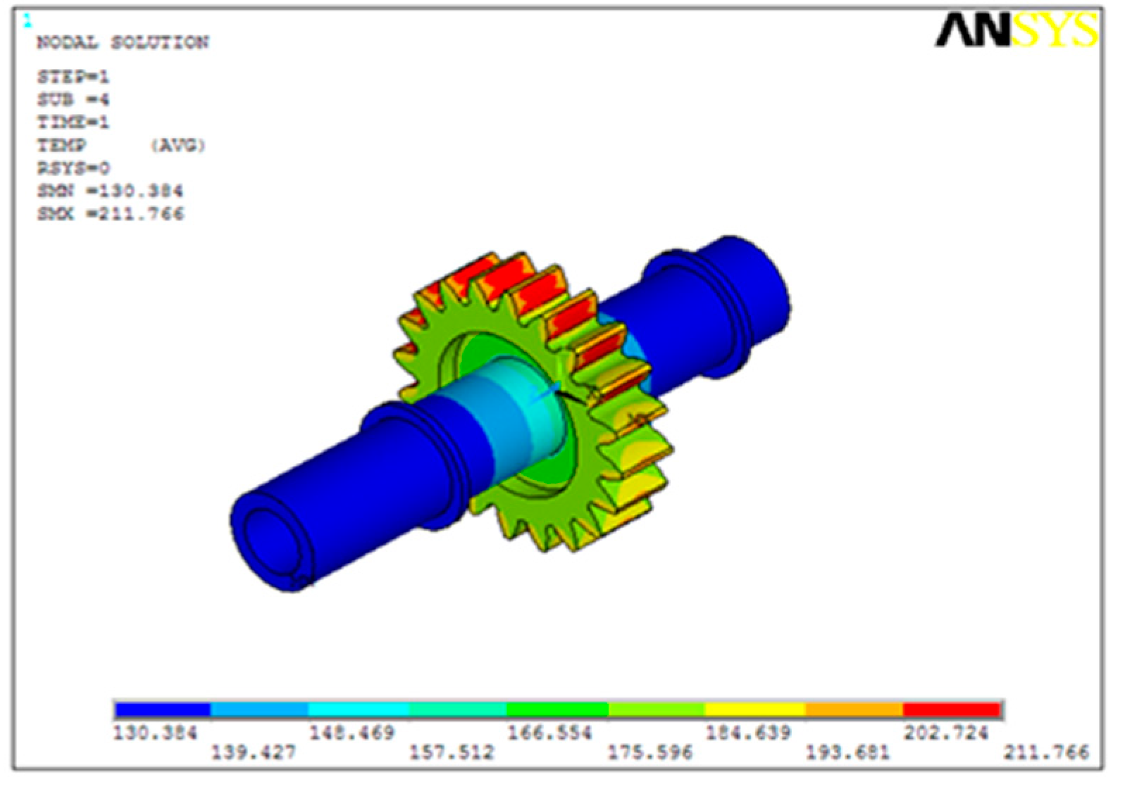
Reasonable mesh density is the guarantee to obtain high precision results. In order to accurately capture the distribution of temperature field, dense mesh should be used in the position with large temperature gradient. To reduce the scale of finite element calculation and improve the analysis efficiency, a relatively sparse grid can be used for the parts with small temperature gradient. Therefore, a relatively dense mesh is used near the meshing tooth surface as shown in Figure 3. The convection heat transfer coefficient and heat flux density are calculated and loaded according to the relevant formula of the 2.2 section. The thermal conductivity of gear is defined as 30.2 W/m3·°C, specific heat capacity 575.6 J/kg·°C and density 7860 kg/m3. The steady-state temperature field distribution is solved, and the data results are saved as .rth file. The temperature field of gear rotor is shown in Figure 4.
Solving the thermal stress is an important step to analyze the gear-rotor natural frequency considering the effect of temperature, which belongs to the thermal—structural coupling analysis. The thermal stress of gear-rotor is solved by load transfer method. Firstly, the load and load step settings of the gear rotor during thermal analysis are cleared, and the element properties are transformed (the thermal analysis element unit Solid70 is transformed into the structural analysis element Solid185). Secondly, the full constraint is applied to both ends of the gear shaft, and the material characteristics that change with temperature are added. Finally, the analysis results of temperature field were read in .rth file to ensure different material properties in different parts, setting the TREF reference temperature to 20 °C, and turn on the pre-stressing switch options.
Since most of the excitation frequencies are concentrated on the first few orders of natural frequencies, only the first six natural frequencies of gear-rotor are considered. In Table 2. The first column i is the order of the natural frequency, the second column f 0 ( i ) indicates the natural frequency without considering the temperature influence, and the third column f 1 ( i ) indicates the natural frequency considering influence of temperature, the fourth column f 1 ( i ) f 0 ( i ) and the fifth column ( f 1 ( i ) f 0 ( i ) ) / f 0 ( i ) represent the difference and percentage in both cases.
From Table 2, the following conclusions can be drawn:
(1) The temperature field has influence on the natural frequency of gear-rotor. The increase in temperature decreases the natural frequency. Because the increase in temperature reduces the material mechanical properties of the gear rotor, the natural frequency of the structure is affected.
(2) The change of temperature reduces the natural frequencies of different orders to different degrees, ranging from tens to hundreds of Hertz. Among the first six natural frequencies, the percentage decreases the most in the first order and the smallest in the sixth order.
When the excitation frequency is close to or equal to the natural frequency, the gear rotor will resonate and cause damage. Therefore, the excitation frequency should be avoided as far as possible from the natural frequency.

4.2. Resonance Failure Analysis of Gear-Rotor

The excitation frequency for generating structural resonance is mainly the meshing frequency of the gear-rotor, and the calculation formula is [2]:
P = nz/60
where z and n are, respectively, the number of gear teeth and the number of revolutions (r/min).
According to the resonance principle, the gear-rotor will resonate when the excitation frequency is close to or equal to the natural frequency. In the manufacturing process of gear rotors, due to the existence of random factors such as manufacturing errors and uneven material, the natural frequency of gear rotor is also uncertain. Temperature changes also affect the natural frequency of the gear-rotor. Since the combined influence of many random factors, the natural frequency of gear-rotor also becomes a random variable. According to reliability interference theory, the performance function of failure analysis of random structures defined as [3]
g i ( p , ω i ) = | p ω i | ( i = 1 , 2 n )
where p is the excitation frequency; ω i is the i-th natural frequency.
The resonance of structural system will cause a large number of responses that do not exceed the threshold value to cause structural failure, which causes the structural system to be in a quasi-failure state, that is, the quasi-failure state that determines the resonance of the structural system is:
g i ( p , ω i ) = | p ω i | γ
where γ is 15% of the natural frequency of each order of the gear-rotor. The mean and variance of the state function are:
μ g i = E ( g i ) = | E ( p ) E ( ω i ) |
σ g i 2 = V a r ( g i ) = σ p 2 + σ ω i 2
The probability of structural system resonance, i.e., quasi-failure probability is:
p f i = p i ( γ p ω i γ )
Assuming that the excitation frequency and the natural frequency, respectively, obey the normal distribution independently, the quasi-failure probability is:
p f i = Φ [ γ μ g i σ g i ] Φ [ γ μ g i σ g i ]
For the gear rotor structure, as long as there is a vibration frequency close to a certain natural frequency, it will make resonance and is considered to be in a failure state. Therefore, the reliability analysis of stochastic structural system based on the natural frequency and excitation frequency of the structural system should be regarded as a series system, and the failure probability of the whole gear-rotor systems can be obtained as follows:
p f = 1 i = 1 n j = 1 m ( 1 p f i j )
The reliability of the whole gear-rotor systems are:
R f = 1 p f = i = 1 n j = 1 m ( 1 p f i j )

4.3. Resonance Reliability Analysis of Gear Rotor

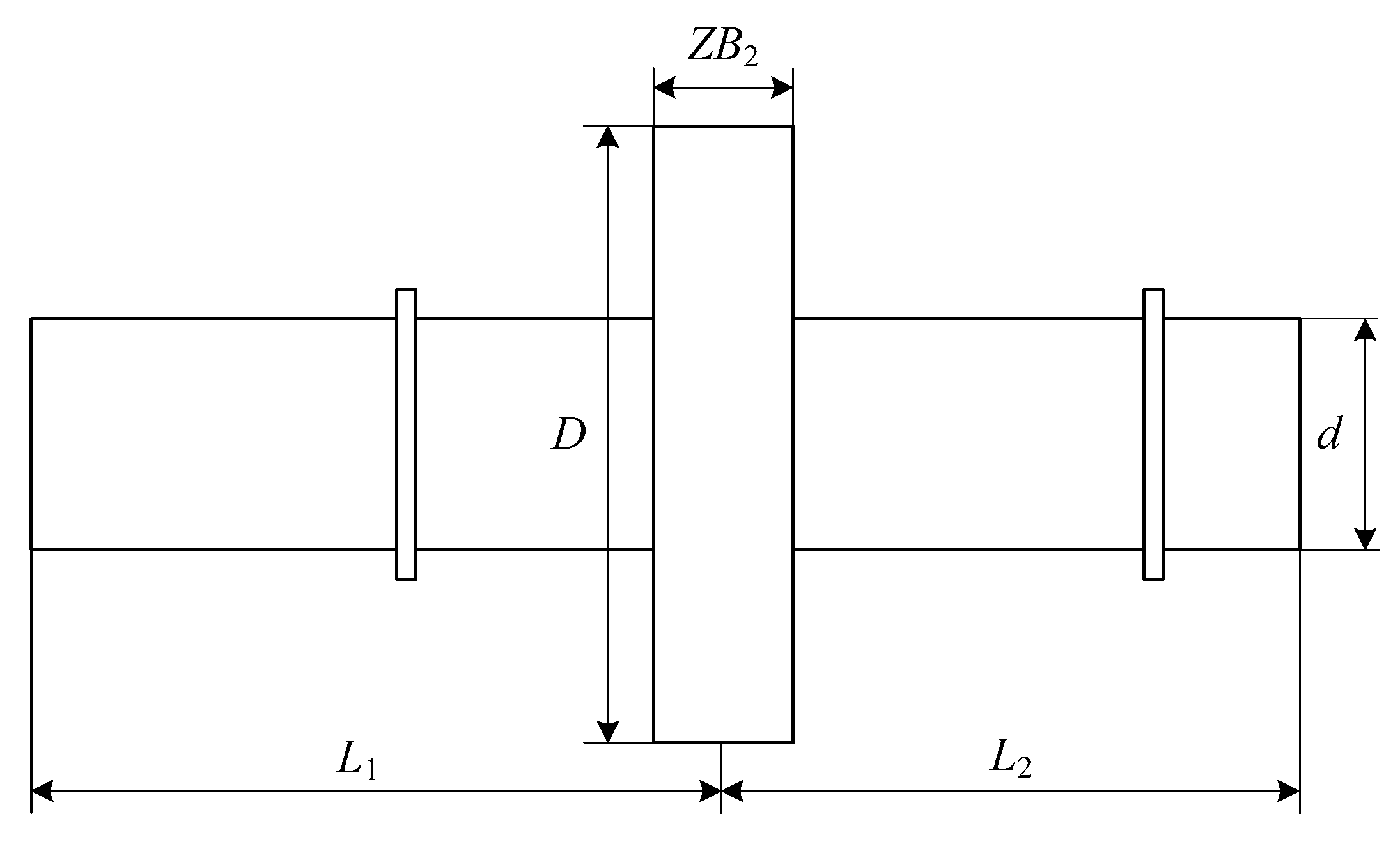
This section will consider both structural dimension parameters and material mechanical properties parameters and will be compiled and executed using APDL. The PC-Kriging method is used to analyze the resonant reliability sensitivity of gear-rotor considering temperature. The two-dimensional dimension variables of the gear-rotor system are shown in Figure 5.
It is assumed that the random parameters of the gear-rotor system size affected by temperature rise are tooth width ZB2, modulus M, shaft length L1, shaft length L2, and tooth width and modulus will also affect the friction heat flux of the gear. The random parameters influencing the mechanical properties of the material are elastic modulus and density of the gear-rotor, and assuming that the excitation frequency of the gear-rotor is also a random parameter. Assume that these parameters are random variables, and that the above random variables are normally distributed. The mean and standard deviation of each random variable are shown in Table 3.

4.4. Resonance Reliability Sensitivity Analysis of Gear Rotor

Reliability sensitivity reflects the influence of random parameters on the gear-rotor reliability. The reliability sensitivity ranking results of random parameters can be obtained through the analysis. It is meaningful to research the influence of statistical characteristics of random parameters (such as mean and standard deviation) on reliability sensitivity.
The reliability sensitivities, with respect to the mean and standard deviation of the random parameters, are written as:
S ( μ g ) = R μ g × μ g R
S ( σ g ) = R σ g × σ g R
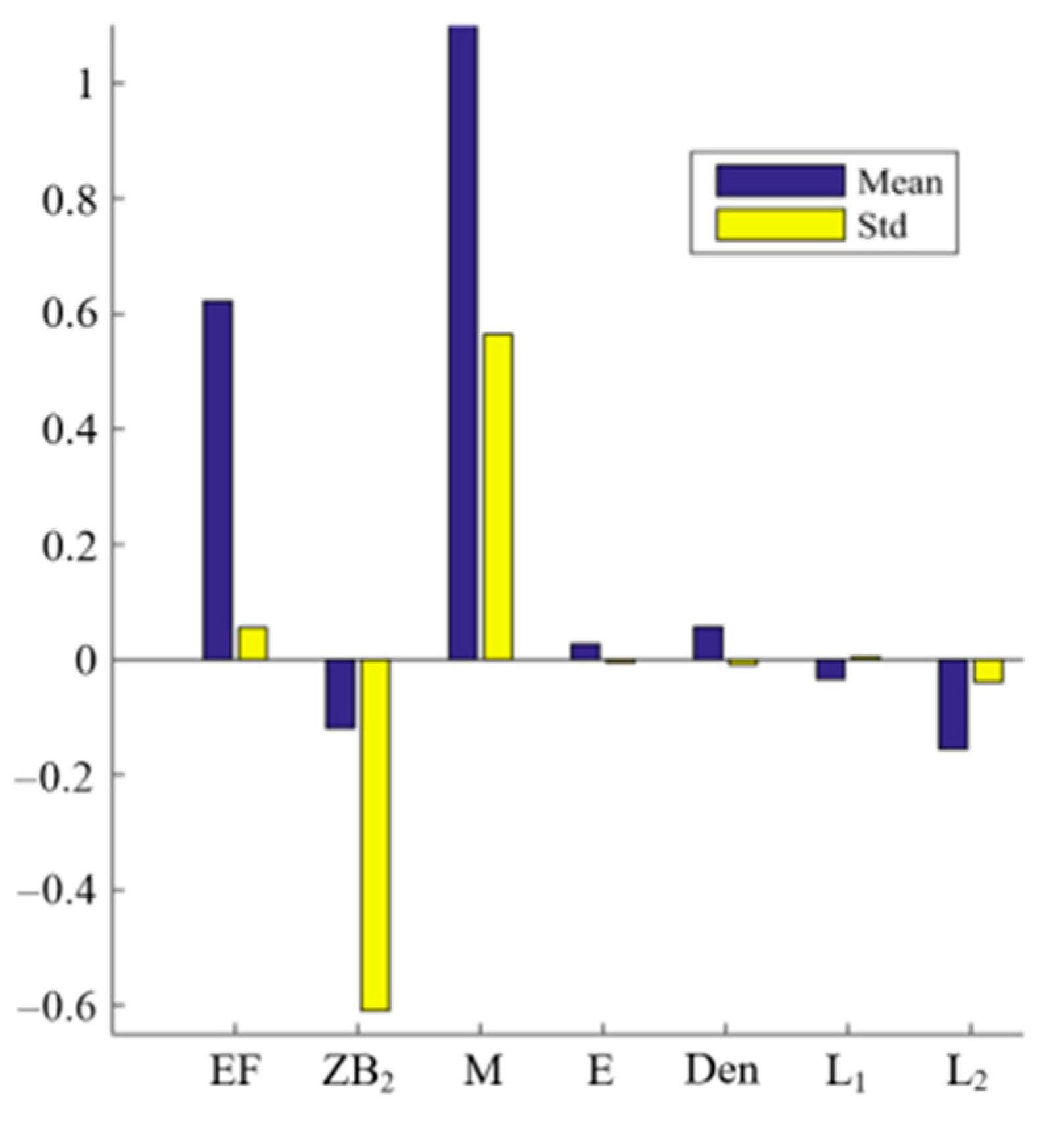
The variation of the random parameters of the gear-rotor system will affect the natural frequency of the rotor, and then affect the resonance reliability of the gear rotor. The influence degree of different parameters is also different. Reliability sensitivity analysis is to calculate the influence of random parameters on reliability, as shown in the histograms Figure 6 and pie charts of Figure 7.
The resonance reliability sensitivity and sensitivity factor of the gear-rotor system are calculated by the above steps. The results are shown in Table 4. The influence of random variables on the resonance reliability of gear-rotor system is shown in cylindrical chart as shown in Figure 6. Resonance reliability is the most sensitive to M, followed by EF and ZB2. E has the least impact. Therefore, in the design process of gear-rotor system, the gear module, tooth width and excitation frequency should be considered, and the improvement and optimization should be made according to the engineering background to ensure that the system has sufficient reliability.
According to the mean sensitivity of each random variable in Figure 6, it is clear that the mean sensitivity of the random variable M is positive, indicating a negative effect on the reliability of the gear rotor resonance. If the mean value of the random variable is increased, the probability of failure increases and the gear system becomes unsafe. The negative mean sensitivity of the random variable ZB2 indicates that the gear rotor has a negative effect on resonance reliability and the effect is positive. If the mean value of the random variable is increased, the probability of failure will decrease, and the gear system will be safe.
As can be seen from the standard variance sensitivity in Figure 6, the standard variance sensitivity of the random variables EF and E is calculated to be positive, indicating that the variance of these two random variables has a negative impact on the reliability of the gear rotor system. If the variance of these two random variables increases, the failure probability of the system increases, and the gear system becomes unsafe. The graph of sensitivity factor weight of each random variable is shown in Figure 7. By analyzing the sensitivity factor specific gravity plot as shown in Figure 7, the degree and trend of influence of each random variable on the resonance reliability of the rotor system can be clearly seen, so that the distribution parameters of these random variables can be understood how to control them.
In the design of gear-rotor, the stochastic parameters which are more sensitive to reliability should be considered, and the random parameters which are less sensitive to reliability can be regarded as deterministic parameters in the design analysis. It can be seen from Figure 6 that among random variables M, ZB2, E and EF, the resonance reliability is most sensitive to the modulus M, followed by EF and ZB2, and E has the least influence. Therefore, it is important to control the design of excitation frequency, modulus, and tooth width parameters of gear in engineering, so as to ensure that the rotor has sufficient resonance reliability.

5. Conclusions

A three-dimensional finite element model of the gear rotor is established, and the intrinsic frequency analysis under thermal-structural coupling is performed. A sensitivity analysis of the resonance reliability of a high-speed heavy-load gear-rotor system considering temperature rise under random parameters is carried out using a combination of PC-Kriging surrogate model and adaptive sampling. The influence of the sensitivity of the mean and variance of different stochastic parameters on the resonance reliability of the geared rotor system is investigated. The main conclusions are as follows:
(1) The temperature rise of the gear-rotor leads to a decrease in the mechanical properties of the material which in turn leads to a decrease in its intrinsic frequency, and the degree to which the intrinsic frequency of each order is affected is different, due to the different temperatures to which each part of the gear-rotor is subjected in the thermal environment, which leads to different changes in the mechanical properties of the material produced by different parts.
(2) Comparing and analyzing the inherent frequency of the gear-rotor with and without considering the temperature, it is found that the increase in the gear temperature will lead to the decrease in the inherent frequency of the gear as a result of the combined effect of both the temperature field and the internal thermal stress of the gear, in which the internal thermal stress of the gear is caused by the temperature gradient and therefore has less influence on the inherent frequency of the gear-rotor.
(3) Through the sensitivity analysis of the resonance reliability of the gear-rotor system, it is found that in order to avoid the occurrence of resonance in the design of the random parameters of the gear should focus on the gear excitation frequency, tooth width and modulus, and improve the optimization and frequency tuning process according to the engineering background, in order to ensure that the system has sufficient reliability.
(4) The influence of the sensitivity of different random parameters on the resonance reliability of the gear system is studied, which provides a strong basis and engineering application value for the design and optimization of the resonance reliability of the gear-rotor system.

Author Contributions

For Conceptualization, methodology, analysis, and writing original draft preparation, Z.Y.; validation, writing review and editing, Z.S.; validation, writing—original draft preparation, S.Z.; writing—original draft preparation, J.W. All authors have read and agreed to the published version of the manuscript.

Funding

The research work financed with the means of Basic Scientific Research Youth Program of Education Department of Liaoning Province, No. LJKQZ2021185; Liaoning Provincial Science and Technology Department Natural Science Foundation Project, No. 2022-YKLH-03; Yingkou Enterprise and Doctor Innovation Program (QB-2021-05); Yingkou Institute of Technology Introduction of doctors to start the fund project (YJRC202109).

Institutional Review Board Statement

Not applicable.

Informed Consent Statement

Not applicable.

Data Availability Statement

Not applicable.

Conflicts of Interest

The authors declare no conflict of interest.

References

  1. Li, W.; Zhai, P.; Tian, J.; Luo, B. Thermal analysis of helical gear transmission system considering machining and installation error. Int. J. Mech. Sci. 2018, 149, 1–17. [Google Scholar] [CrossRef]
  2. Qiu, J.; Zhang, J.; Ma, Y. Resonance Reliability Sensitivity Analysis for Torsional Vibration of Gear-Rotor Systems with Random Parameters. In Proceedings of the ASME 2017 International Mechanical Engineering Congress and Exposition, Tampa, FL, USA, 3–9 November 2017; Volume 14, pp. 121–131. [Google Scholar]
  3. Su, C.; Guo, F.; Shi, Q.; Zhang, Y. Reliability sensitivity estimation of rotor system with oil whip and resonance. Adv. Mech. Eng. 2017, 9, 168–180. [Google Scholar] [CrossRef] [Green Version]
  4. Zhou, J.; Zhu, S.; Qiu, Y.; Armaghani, D.J.; Zhou, A.; Yong, W. Predicting tunnel squeezing using support vector machine optimized by whale optimization algorithm. Acta Geotech. 2022, 17, 1343–1366. [Google Scholar] [CrossRef]
  5. Wu, J.; Wang, Z. A Hybrid Model for Water Quality Prediction Based on an Artificial Neural Network, Wavelet Transform, and Long Short-Term Memory. Water 2022, 14, 610. [Google Scholar] [CrossRef]
  6. Liu, J.; Huang, Q.; Ulishney, C.; Dumitrescu, C.E. Comparison of Random Forest and Neural Network in Modeling the Performance and Emissions of a Natural Gas Spark Ignition Engine. J. Energy Resour. Technol. 2022, 144, 032310. [Google Scholar] [CrossRef]
  7. Yang, Y.; Li, X.; Gu, Y.; Lin, H.; Jie, B.; Zhang, Q.; Zhang, X. Adsorption property of fluoride in water by metal organic framework: Optimization of the process by response surface methodology technique. Surf. Interfaces 2022, 28, 101649. [Google Scholar] [CrossRef]
  8. Saeed, A.A.H.; Harun, N.Y.; Nasef, M.M.; Al-Fakih, A.; Ghaleb, A.A.S.; Afolabi, H.K. Removal of cadmium from aqueous solution by optimized rice husk biochar using response surface methodology. Ain Shams Eng. J. 2022, 13, 101516. [Google Scholar] [CrossRef]
  9. Wang, Z.; Shafieezadeh, A. Metamodel-based subset simulation adaptable to target computational capacities: The case for high-dimensional and rare event reliability analysis. Struct. Multidiscip. Optim. 2021, 64, 649–675. [Google Scholar] [CrossRef]
  10. Zhang, C.; Wang, Z.; Shafieezadeh, A. Value of Information Analysis via Active Learning and Knowledge Sharing in Error-Controlled Adaptive Kriging. IEEE Access 2020, 99, 51021–51034. [Google Scholar] [CrossRef]
  11. Song, C.; Wang, Z.; Shafieezadeh, A.; Xiao, R. BUAK-AIS: Efficient Bayesian Updating with Active learning Kriging-based Adaptive Importance Sampling. Comput. Methods Appl. Mech. Eng. 2022, 391, 114578. [Google Scholar] [CrossRef]
  12. Xiao, X.; Li, Q.; Wang, Z. A novel adaptive importance sampling algorithm for Bayesian model updating. Struct. Saf. 2022, 97, 102230. [Google Scholar] [CrossRef]
  13. Wang, Z.; Shafieezadeh, A.; Xiao, X.; Wang, X.; Li, Q. Optimal monitoring location for tracking evolving risks to infrastructure systems: Theory and application to tunneling excavation risk. Reliab. Eng. Syst. Saf. 2022, 228, 108781. [Google Scholar] [CrossRef]
  14. Zhang, H.; Song, L.K.; Bai, G.C.; Li, X.Q. Active extremum Kriging-based multi-level linkage reliability analysis and its application in aeroengine mechanism systems. Aerosp. Sci. Technol. 2022, 131, 107968. [Google Scholar] [CrossRef]
  15. Li, X.Q.; Song, L.K.; Bai, G.C. Vectorial surrogate modeling approach for multi-failure correlated probabilistic evaluation of turbine rotor. Eng. Comput. 2021, 12, 1–20. [Google Scholar] [CrossRef]
  16. Li, X.Q.; Song, L.K.; Bai, G.C. Recent advances in reliability analysis of aeroengine rotor system: A review. Int. J. Struct. Integrity. 2022, 13, 1–29. [Google Scholar] [CrossRef]
  17. Bucher, C.; Most, T. A comparison of approximate response functions in structural reliability analysis. Probabilistic Eng. Mech. 2008, 23, 154–163. [Google Scholar] [CrossRef]
  18. Schoebi, R.; Sudret, B.; Wiart, J. Polynomial-Chaos-Based Kriging. Int. J. Uncertain. Quantif. 2015, 5, 171–193. [Google Scholar] [CrossRef] [Green Version]
  19. Handschuh, R.F. Thermal Behavior of Spiral Bevel Gears. Ph.D. Thesis, Case Western Reserve University, Cleveland, OH, USA, 1993. [Google Scholar]
  20. Shi, Y.; Yao, Y.-P.; Fei, J.-Y. Analysis of bulk temperature field and flash temperature for locomotive traction gear. Appl. Therm. Eng. 2016, 99, 528–536. [Google Scholar] [CrossRef]
  21. Wang, Y.; Tang, W.; Chen, Y.; Wang, T.; Li, G.; Ball, A.D. Investigation into the meshing friction heat generation and transient thermal characteristics of spiral bevel gears. Appl. Therm. Eng. 2017, 119, 245–253. [Google Scholar] [CrossRef]
  22. Dewinter, A.; Blok, H. Fling-Off Cooling of Gear Teeth. J. Eng. Ind. 1974, 96, 60–72. [Google Scholar] [CrossRef]
  23. Long, H.; Lord, A.A.; Gethin, D.T.; Roylance, B.J. Operating temperatures of oil-lubricated medium-speed gears: Numerical models and experimental results. Proc. Inst. Mech. Eng. Part Gs J. Aerosp. Eng. 2003, 217, 87–106. [Google Scholar] [CrossRef] [Green Version]
  24. Van Heijningen, G.J.J.; Blok, H. Continuous as Against Intermittent Fling-Off Cooling of Gear Teeth. J. Lubr. Technol. 1974, 96, 529–538. [Google Scholar] [CrossRef]
  25. Patir, N.; Cheng, H.S. Prediction of the Bulk Temperature in Spur Gears Based on Finite Element Temperature Analysis. ASLE Trans. 1979, 22, 25–36. [Google Scholar] [CrossRef]
  26. Hartnett, J.P.; Deland, E.C. The Influence of Prandtl Number on the Heat Transfer from Rotating Nonisothermal Disks and Cones. J. Heat Transf. 1961, 83, 95–96. [Google Scholar] [CrossRef]
  27. Popiel, C.; Bogusławski, L. Local heat-transfer coefficients on the rotating disk in still air. Int. J. Heat Mass Transf. 1975, 18, 167–170. [Google Scholar] [CrossRef]
  28. Dorfman, L.A.; Kemmer, N. Hydrodynamic Resistance and the Heat Loss of Rotating Solids; Oliver & Boyd: Edinburgh, UK, 1963. [Google Scholar]
  29. Fernandes, C.M.; Rocha, D.M.; Martins, R.C.; Magalhães, L.; Seabra, J.H. Finite element method model to predict bulk and flash temperatures on polymer gears. Tribol. Int. 2018, 120, 255–268. [Google Scholar] [CrossRef]
  30. Anderson, J.T.; Saunders, O.A. Convection from an isolated heated horizontal cylinder rotating about its axis. Proc. R. Soc. Lond. Ser. A Math. Phys. Sci. 1953, 217, 555–562. [Google Scholar]
  31. Becker, K.M. Measurements of convective heat transfer from a horizontal cylinder rotating in a tank of water. Int. J. Heat Mass Transf. 1963, 6, 1053–1062. [Google Scholar] [CrossRef]
  32. Seghir-Ouali, S.; Saury, D.; Harmand, S.; Phillipart, O.; Laloy, D. Convective heat transfer inside a rotating cylinder with an axial air flow. Int. J. Therm. Sci. 2006, 45, 1166–1178. [Google Scholar] [CrossRef]
  33. Luo, B.; Li, W. Influence factors on bulk temperature field of gear. Proc. Inst. Mech. Eng. Part J J. Eng. Tribol. 2017, 231, 953–964. [Google Scholar] [CrossRef]
  34. Efron, B.; Hastie, T.; Johnstone, I.; Tibshirani, R. Least angle regression. Ann. Stat. 2004, 32, 407–499. [Google Scholar] [CrossRef]
  35. Arnold, T.W. Uninformative Parameters and Model Selection Using Akaike’s Information Criterion. J. Wildl. Manag. 2011, 74, 1175–1178. [Google Scholar] [CrossRef]
  36. Tenebaum, J.B. A global geometric framework for nonlinear dimensionality reduction. Science 2000, 290, 2319–2323. [Google Scholar] [CrossRef] [PubMed]
  37. Macqueen, J. Some Methods for Classification and Analysis of MultiVariate Observations. In Proceedings of the Fifth Berkeley Symposium on Mathematical Statistics and Probability, Berkeley, CA, USA, 21 June–18 July 1965 and 27 December 1965–7 January 1966. [Google Scholar]
  38. Saxena, A.; Chouksey, M.; Parey, A. Measurement of FRFs of coupled geared rotor system and the development of an accurate finite element model. Mech. Mach. Theory 2018, 123, 66–75. [Google Scholar] [CrossRef]
  39. Concli, F.; Cortese, L.; Vidoni, R.; Nalli, F.; Carabin, G. A mixed FEM and lumped-parameter dynamic model for evaluating the modal properties of planetary gearboxes. J. Mech. Sci. Technol. 2018, 32, 3047–3056. [Google Scholar] [CrossRef]
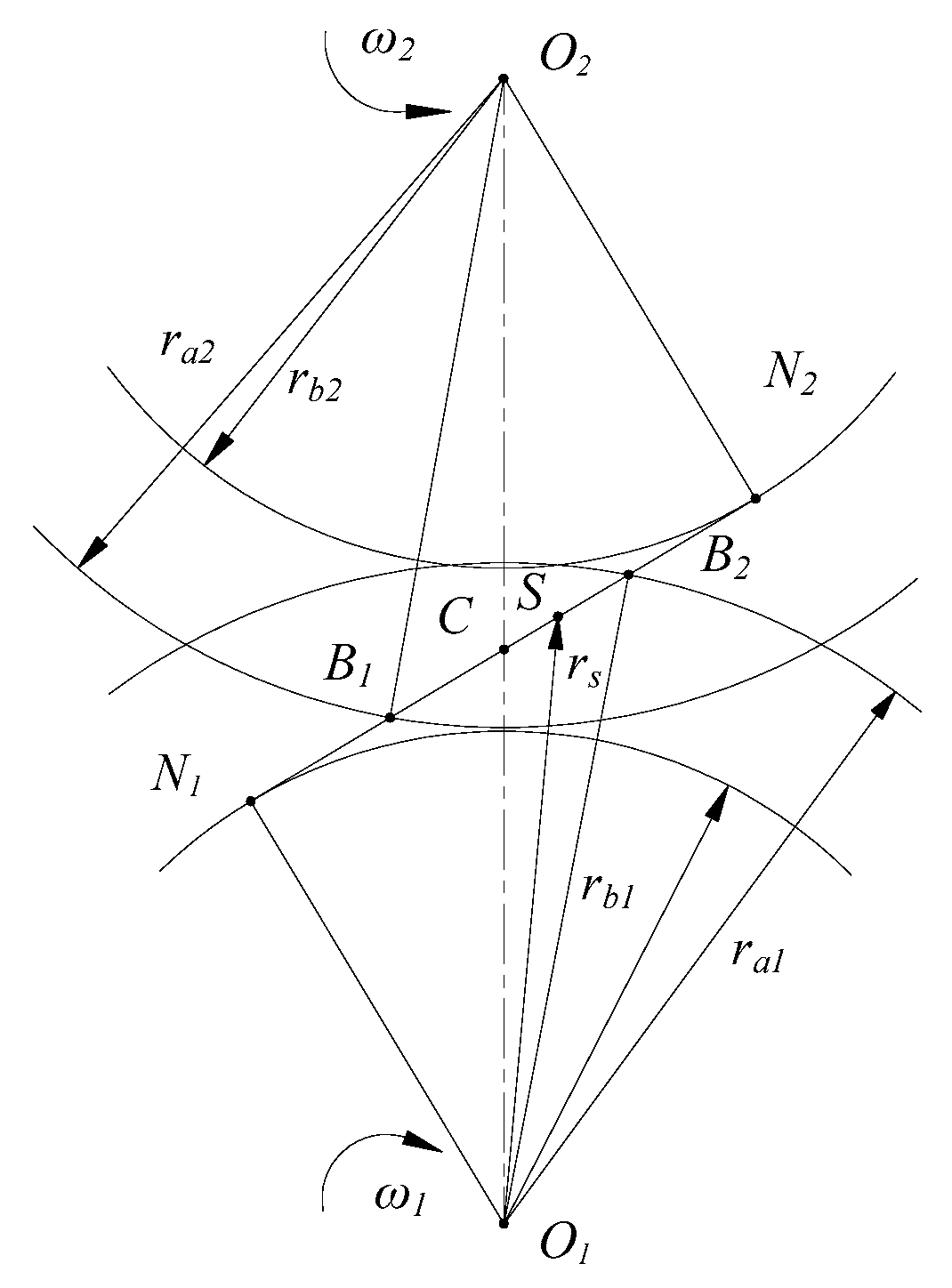
Figure 1. Transmission process of spur gear.
Sustainability 15 00255 g001
Figure 2. Calculation region of single gear tooth.
Sustainability 15 00255 g002
Figure 3. Gear-rotor model after meshing.
Sustainability 15 00255 g003
Figure 4. Temperature field contours.
Sustainability 15 00255 g004
Figure 5. Two-dimensional dimension variables.
Sustainability 15 00255 g005
Figure 6. Sensitivity of random variables.
Sustainability 15 00255 g006
Figure 7. Ratio of Sensitivity Factor.
Sustainability 15 00255 g007
Table 1. The basic parameters of gear.
Basic ParametersDriving GearsDriven Gears
Module33
Number of teeth3420
pressure angle (°)2525
Face width (mm)1514.5
Addendum coefficient11
Coefficient of clearance0.250.25
Modification coefficient00
Radius of gear spoke (mm)4020
Gear spoke width (mm)65
Table 2. Contrast of the first 6 natural frequencies.
Order i f 0 ( i ) f 1 ( i ) f 1 ( i ) f 0 ( i ) ( f 1 ( i ) f 0 ( i ) ) / f 0 ( i )
142634181−82−1.92%
257225665−57−1.00%
357225665−57−1.00%
461826123−59−0.95%
561846125−59−0.95%
683578333−24−0.29%
Table 3. Mean and standard deviation of all random variation.
EF (Hz)ZB2 (mm)M (mm)E (MPa)Den (kg/m3)L1 (mm)L2 (mm)
Means4533.3314.532.1 × 10578601440
Std45.30.290.03756.3 × 10378.60.72
Table 4. Sensitivity of the gear rotor to random parameters.
ParameterEFZB2MEDenL1L2
Mean0.6224−0.11891.12970.02760.0570−0.0335−0.1553
Std0.0554−0.60900.5645−0.0047−0.00810.0049−0.0389
Factor0.22410.22260.45300.01000.02070.01210.0574
Disclaimer/Publisher’s Note: The statements, opinions and data contained in all publications are solely those of the individual author(s) and contributor(s) and not of MDPI and/or the editor(s). MDPI and/or the editor(s) disclaim responsibility for any injury to people or property resulting from any ideas, methods, instructions or products referred to in the content.