A Chaotic Search-Based Hybrid Optimization Technique for Automatic Load Frequency Control of a Renewable Energy Integrated Power System

Abstract

In this work, a chaotic search-based hybrid Sperm Swarm Optimized-Gravitational Search Algorithm (CSSO-GSA) is proposed for automatic load frequency control (ALFC) of a hybrid power system (HPS). The HPS model is developed using multiple power sources (thermal, bio-fuel, and renewable energy (RE)) that generate power to balance the system’s demand. To regulate the frequency of the system, the control parameters of the proportional-integral-derivative (PID) controller for ALFC are obtained by minimizing the integral time absolute error of HPS. The effectiveness of the proposed technique is verified with various combinations of power sources (all sources, thermal with bio-fuel, and thermal with RE) connected into the system. Further, the robustness of the proposed technique is investigated by performing a sensitivity analysis considering load variation and weather intermittency of RE sources in real-time. However, the type of RE source does not have any severe impact on the controller but the uncertainties present in RE power generation required a robust controller. In addition, the effectiveness of the proposed technique is validated with comparative and stability analysis. The results show that the proposed CSSO-GSA strategy outperforms the SSO, GSA, and hybrid SSO-GSA methods in terms of steady-state and transient performance indices. According to the results of frequency control optimization, the main performance indices such as settling time (ST) and integral time absolute error (ITAE) are significantly improved by 60.204% and 40.055% in area 1 and 57.856% and 39.820% in area 2, respectively, with the proposed CSSO-GSA control strategy compared to other existing control methods.

1. Introduction

Nowadays, the interconnected power system has evolved into a complex network that faces the issue of maintaining the generation-load balance at all times in order to achieve frequency regulation. With the goal of limiting fossil fuel depletion and reducing carbon emissions, it is urged to increase the penetration of renewable energy sources in the network, which may impair system stability and increase frequency/tie-line power aberrations. In order to address this issue, each control region of an interconnected power system employs an automatic generation control (AGC) or automatic load frequency control (ALFC) to maintain the generation-load balance during severe disturbances [1,2].

For ALFC applications, several researchers have looked into traditional classical controllers like proportional–integral (PI), proportional–integral–derivative (PID), proportional–derivative (PD), and integral–double–derivative (IDD) controllers [3,4]. The analysis of these controllers demonstrates that the design of the control model is heavily reliant on mathematical modeling, and their performances are not effective for the dynamic system with non-linearities (governor dead-band (GDB) and generator rate constraint (GRC)) [5]. Furthermore, various control methods like the internal model control (IMC), variable structure control [6], linear quadratic optimal control [7], H₂/H∞ robust control, model predictive control, linear matrix control, and fractional order (FO) control [8] have been applied by the researchers to solve the ALFC problem under dynamic conditions of a power system. For most control applications, the PID controller is extensively used due to its simplicity and easy implementation. However, with traditional tuning methods, optimizing the gains of the PID controller is one of the most important tasks to achieve improved dynamic and steady-state responses of the control system. This can be resolved by optimizing the control gains of a controller with various intelligent techniques such as fuzzy [9], artificial neural network (ANN) [10], and adaptive neuro-fuzzy inference system (ANFIS) [11]. However, these control schemes necessitate a significant amount of time to formulate the rules and train the network [12]. As a result, to overcome the problems of these control methods, many researchers have used various heuristic-based stochastic optimization techniques such as genetic algorithm (GA), gravitational search algorithm (GSA), firefly algorithm (FA), artificial bee colony, (ABC), particle swarm optimization (PSO), Cuckoo search (CS), Grey Wolf Optimization (GWO), teaching learning-based optimization (TLBO), dragon fly optimization (DFO), differential evaluation (DE), etc., to tune the control gains of the PID controller for the ALFC application [13,14]. Also, the performance of these algorithms may degrade for the power system operating with a different generation system coupled with its mechanical devices that required retuning of the controller gains as the configuration of the system operation changes. Hence, hybrid techniques are essential in tuning the gains of the controller, as they have a better exploration and exploitation search capability compared to other specified methods.

In the case of the system associated with large dynamics, the control gains obtained from the aforementioned algorithms are ineffective in reducing the system error by reaching local minima. In this context, a meta-heuristic algorithm that integrates the exploration (searching ability) and exploitation (global best) characteristics of several optimization methods was used to increase the efficiency of the controllers by approaching the global optimal solution [15]. Several hybrid algorithms such as PSO-GA, PSO-DE, PSO with Artificial Bee Colony, namely PSO-ABC, and GWO with Cuckoo Search algorithm, namely GWO-CS, are implemented by the researchers to achieve better speed of convergence control and quality of a solution by appropriately tuning the controllers [16,17]. PSO-based hybrid algorithms are extensively used because they are simple and can achieve a better speed of convergence than other state-of-the-art hybrid optimization techniques. The PSO-GSA based hybrid optimization strategy was used to tune the PID controller for the ALFC application in [15,16], and had a faster convergence rate with a better dynamic and steady-state control responsiveness than standard optimization methods.

In this work, a new hybrid optimization technique using the most recent sperm swarm optimization (SSO) algorithm with a GSA approach, namely SSO-GSA, is proposed to tune the control gains of the PID controller for the ALFC of the two-area interconnected power system (TAIPS) under various dynamic conditions. The SSO is a swarm-based optimization method inspired by sperm swarm activity during natural fertilization [18,19] and has the following unique characteristics: high precision of exploitation ability, faster convergence with the ability to find a global optimum, simple computations, and easy implementation. Similarly, GSA is a physics-based optimization technique inspired by Newton’s theory of gravity [20] that offers the following benefits: high precision of exploration capability, simple and easy implementation, applicable to real-time problems, and the ability to solve non-parametric, non-differential, and multi-dimensional problems [21,22,23]. Through merging of SSO’s exploitation skills with GSA’s exploration capabilities, the proposed hybrid technique (SSO-GSA) provides the strengths of both GSA and SSO algorithms. As a result, the proposed approach will be able to search and explore any search space domain with a fast convergence rate and better optimum solution.

Furthermore, the performance of metaheuristic optimization algorithms can also be improved with the implementation of chaos theory, which is the most recent popular application with the following unique characteristics: dynamicity, ergodicity, and non-repetitively [24,25,26]. The dynamic property of chaos theory ensures that the algorithm investigates different landscapes in the search space and delivers a variety of solutions, while ergodicity and non-repetition speed up the search [26]. The literature of chaos theory application with different optimization algorithms such as the crow search algorithm (CSA) [27], salp swarm algorithm (SSA) [28], GWO [29], GA [30], grasshopper optimization algorithm (GOA) [31], firefly algorithm (FA) [32], imperialist competitive algorithm (ICA), and incremental learning algorithm (ICL) [33] clearly show that the chaotic sequence of mapping (1D map method) application works well (than random variables) and improves the global convergence speed along with the exploration/exploitation capabilities of optimization algorithms [34]. Therefore, in this study, in order to improve the performance of the hybrid SSO-GSA optimization technique in terms of dynamic and steady-state responses, a chaotic search has been incorporated into the hybrid optimization technique, SSO-GSA, using a 1D chaotic map and validated for the ALFC application. The proposed chaotic-based hybrid technique improves the overall performance while verifying different bench mark functions with standard SSO, GSA, and hybrid SSO-GSA methods.

The salient contributions of this study are outlined as follows:

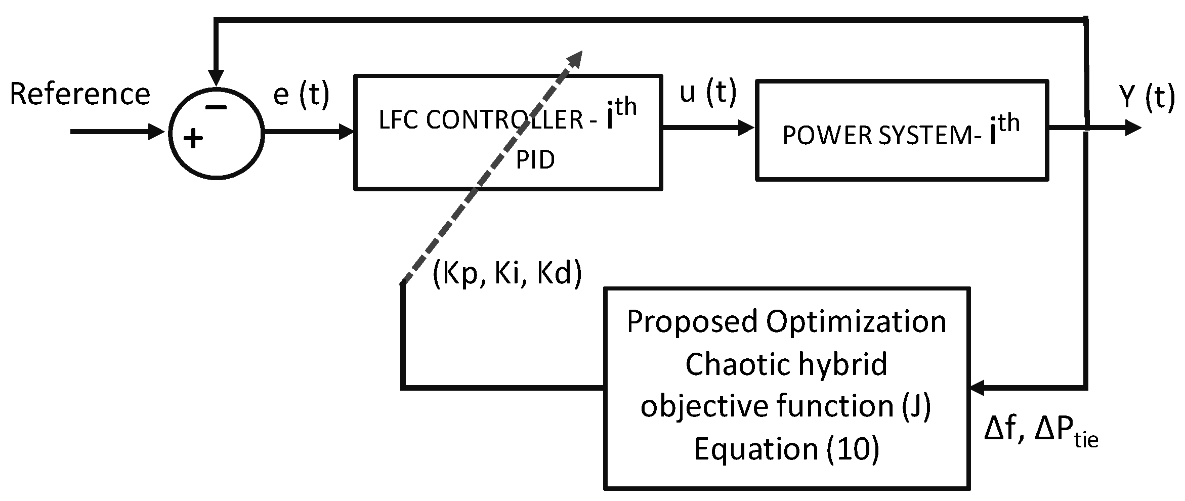
• A chaotic-based (1D mapping sequence) hybrid SSO-GSA optimization technique is implemented to optimize the parameters of the PID controller for ALFC of HPS.
• A dynamic condition of comprehensive analysis is carried out for the proposed CSSO-GSA technique under different combinations of power sources interconnected into the TAIPS.
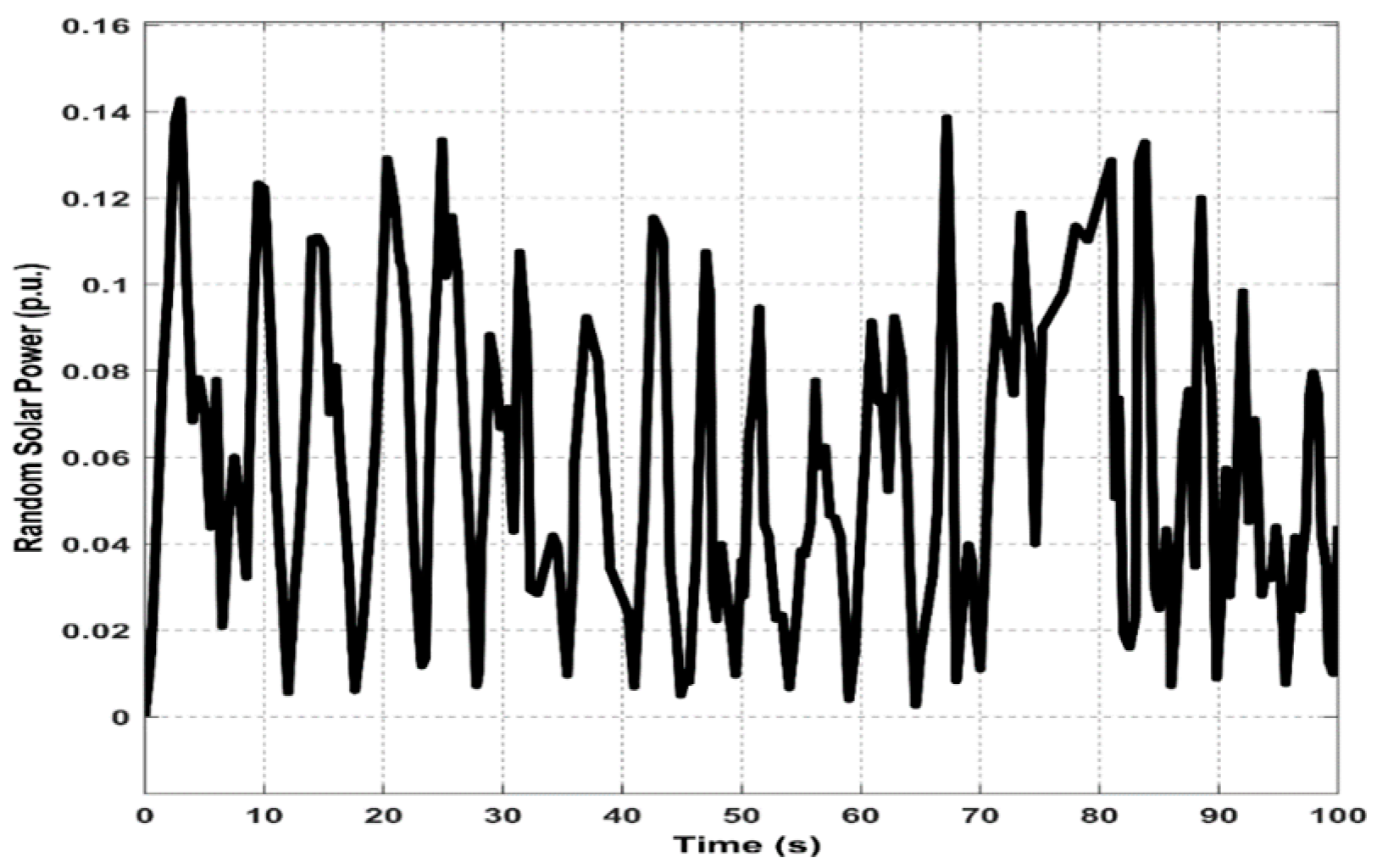
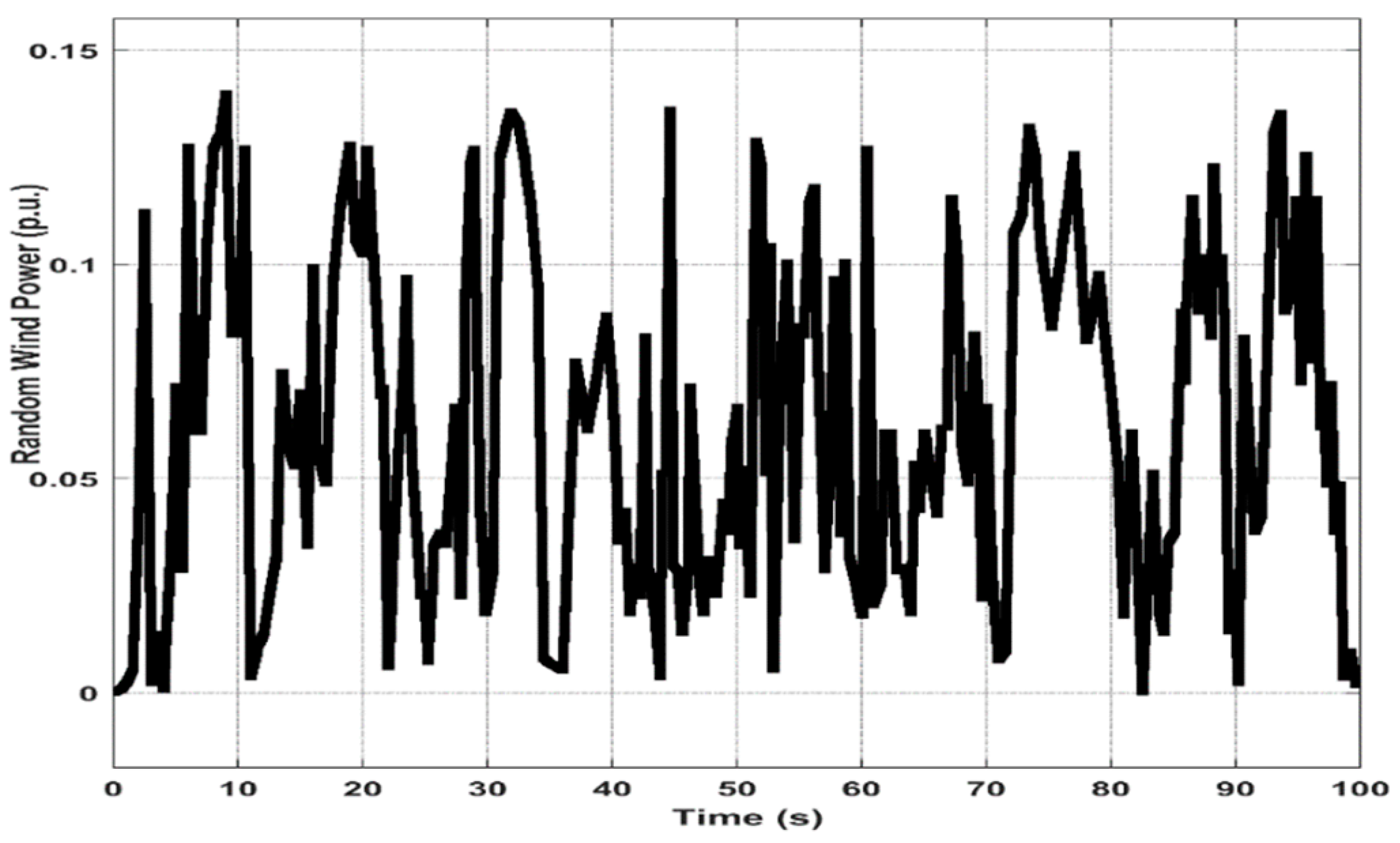
• Sensitivity analysis is carried out under load disturbance and varying (wind and solar) power conditions in real time in order to study the robustness of the proposed CSSO-GSA technique.
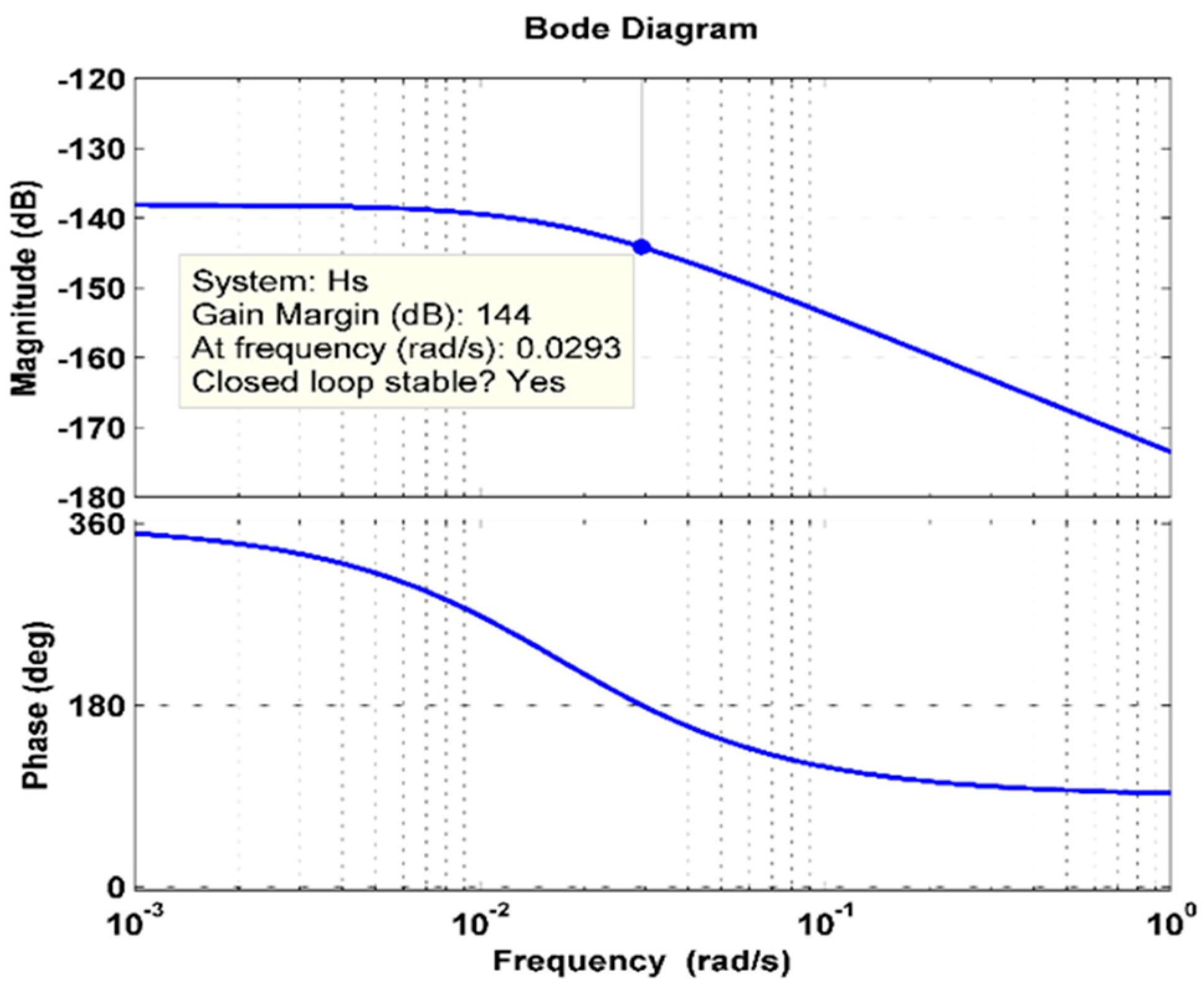
• A stability analysis was performed to explore the frequency stability of the HPS model.
• A comparative analysis with a literature study is conducted to validate the performance of the proposed CSSO-GSA control technique and to exhibit its global convergence ability.

The paper is structured as follows: Section 2 describes the interconnected HPS model with integration of multi-power sources including conventional power (thermal), bio-power (bio-gas and bio-diesel), RE sources (solar thermal and wind power), and energy storage devices (aqua electrolyzer (AE) and fuel cell (FC)). Section 3 details the control scheme and optimization algorithms of SSO, GSA, and proposed hybrid SSO-GSA, along with implementation of the chaotic technique; Section 4 presents the results and discussion of HPS simulation with various case studies and sensitivity analysis; Section 5 concludes the outcomes of the proposed work.

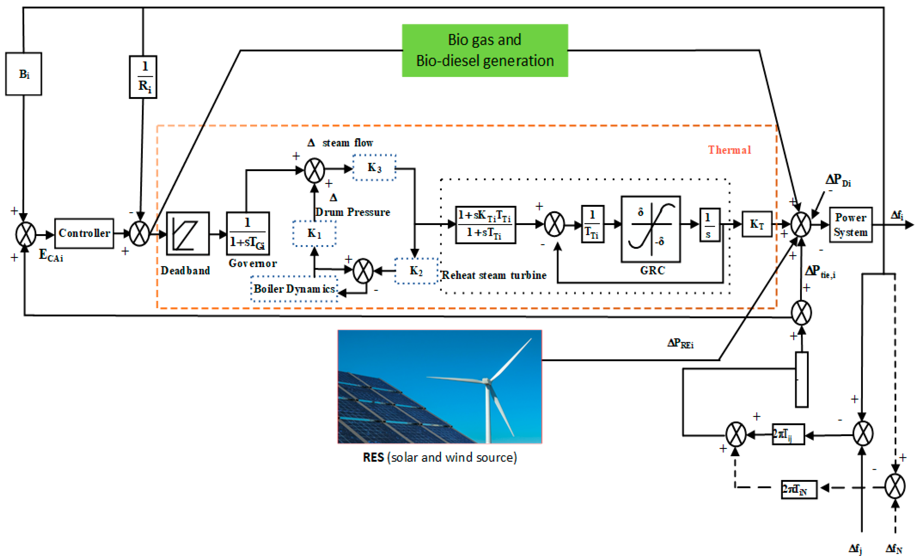
2. Two-Area Interconnected Power System (TAIPS) Model

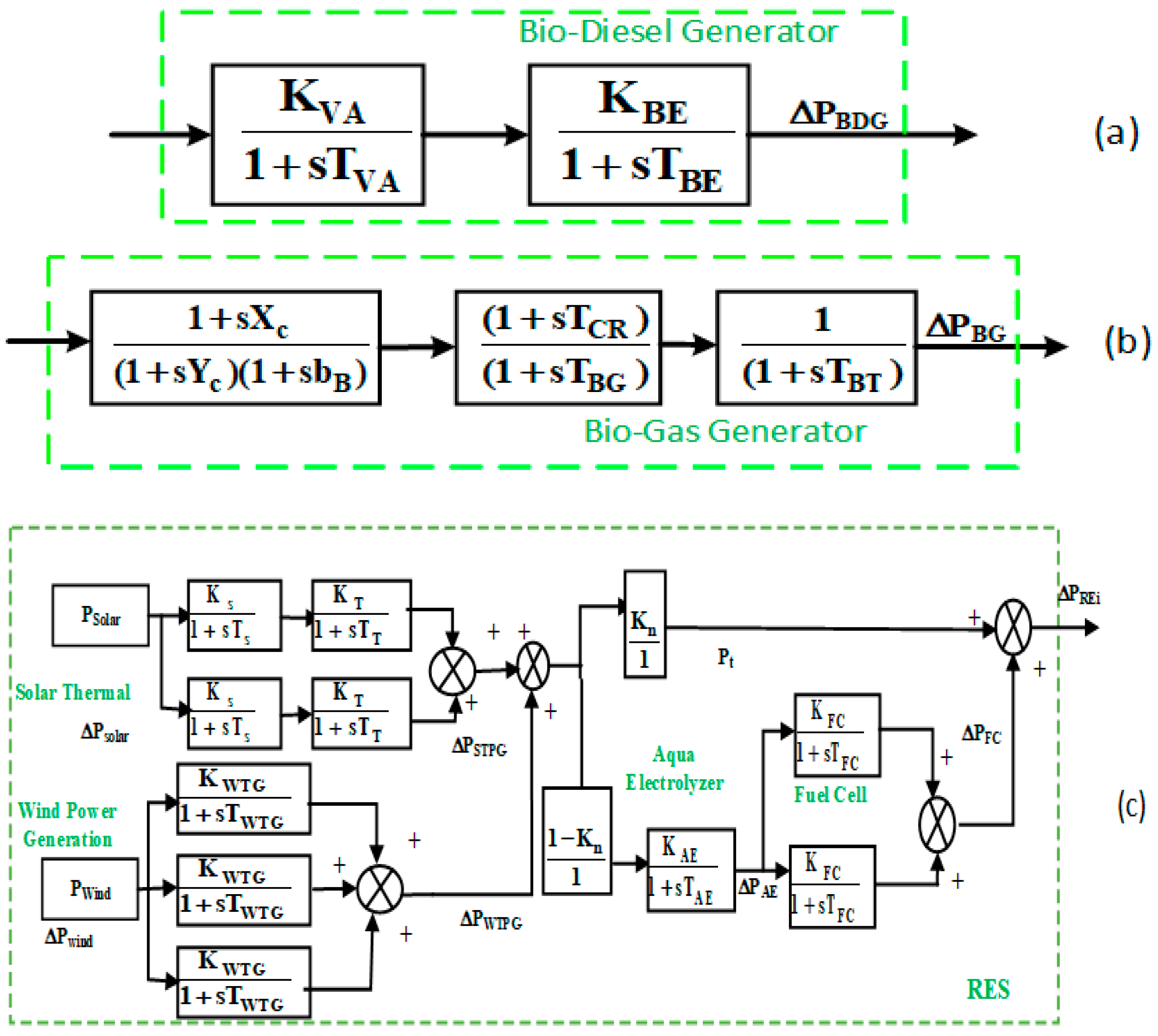
The schematic diagram of two-area HPS, which is shown in Figure 1, consists of the following sources: thermal power reheat unit, bio-power (bio-gas (Figure 2a and bio diesel (Figure 2b), RE sources (solar thermal power and wind power (Figure 2c), and energy storage sources (AE and FC (Figure 2c)). The parameters for the reheat thermal power generation units are considered as per the explanation given in the literature [11,15]. The details for the remaining sources of the HPS model are given as follows:

2.1. RE Sources

The solar thermal power source (STPS) and wind turbine generation source (WTGS) models are considered as RE sources in this HPS network model. The STPS model consists of a solar collector and a steam turbine generating unit. The STPS model is linearized with a few approximations and the first-order transfer function for that model is given as [35],

$$G_s\left(s\right)=\frac{\Delta P_{STPG}}{\Delta P_{solar}}=\frac{K_s}{1+s{T}_s}\times \frac{K_T}{1+s{T}_T}$$

(1)

Considering the dynamics of the WTGS model, the first order transfer function of the model can be written as [36],

$$G_{WTG}\left(s\right)=\frac{\Delta P_{WTPG}}{\Delta P_{wind}}=\frac{K_{WTG}}{1+s{T}_{WTG}}$$

(2)

2.2. Bio Power Sources

The bio-gas and bio-diesel plant models are considered as bio-power sources in the HPS network. The linearized first-order transfer function of bio-gas and bio-diesel plant models are expressed in Equations (3) and (4), respectively, as given below [37]:

$$G_{bg}\left(s\right)=\frac{1+s{X}_C}{\left(1+s{Y}_C\right)\left(1+s{b}_B\right)}\times \frac{1+s{T}_{CR}}{1+s{T}_{BG}}\times \frac{K_{BT}}{1+s{T}_{BT}}$$

(3)

$$G_{bd}\left(s\right)=\frac{K_{BA}}{1+s{T}_{BA}}\times \frac{K_{BE}}{1+s{T}_{BE}}$$

(4)

2.3. Energy Storage

The HPS model incorporates energy storage devices such as an aqua electrolyzer (AE) and fuel cell (FC) to suppress any power variation from RE sources. With AE, excess power generated by RE sources can be used to produce hydrogen (H₂) and store it. In the case of power fluctuations in RE sources or low power yields (due to low wind and solar power), the stored H₂ can be used by the FC to generate power. The first-order transfer function for non-linear models of AE and FC is defined in the following Equations (5) and (6), respectively [35].

$$G_{AE}\left(s\right)=\frac{K_{AE}}{1+s{T}_{AE}}=\frac{\Delta P_{AE}}{\left(\Delta P_{WTG}+\Delta P_{STPG}\right)\left(1-K_n\right)}$$

(5)

where $K_n=\frac{P_t}{\left(P_{WTG}+P_{STPG}\right)}$ is assumed as 0.6,

$$G_{FC}\left(s\right)=\frac{K_{FC}}{1+s{T}_{FC}}$$

(6)

The gain and time constant values for the transfer function of various power sources, and values of other factors used in power system, are given in Appendix A.

3. Control System

The PID controller is widely used in most control applications due to its simplicity and easy implementation. The transfer function of the PID controller can be expressed in the s-domain as [38],

$$G_{\mathrm{PID}}\left(s\right)=\frac{\mathrm{E} \left(\mathrm{S}\right)}{\mathrm{U}\left(\mathrm{S}\right)}={\mathrm{K}}_p+{\mathrm{K}}_{i}s+\frac{{\mathrm{K}}_d}{\mathrm{S}}$$

(7)

where U (S) is the controller output signal, E (S) is the tracking error signal, K_P, K_I, and K_D are the controller’s proportional, integral, and derivative gains. The closed loop feedback control with tuning parameters of controllers for each area of the system is shown in Figure 1. Considering the given set value (Y_ref), actual plant output (Y_plant), and error signal e (t) of a closed loop feedback control system, the u (t) of controller output in each area can be expressed as follows [15]:

Considering for Area 1

$${\mathrm{U}}_1 (\mathrm{t})={\mathrm{K}}_{\mathrm{P}1}{\mathrm{ACE}}_1+{\mathrm{K}}_{\mathrm{I}1} {{\displaystyle \int }}_0^T{\mathrm{ACE}}_1\mathrm{dt}+K_{d1}\frac{{\mathrm{dACE}}_1}{\mathrm{dt}}$$

(8)

Considering for Area 2

$${\mathrm{U}}_2 (\mathrm{t})={\mathrm{K}}_{\mathrm{P}2}{\mathrm{ACE}}_2+{\mathrm{K}}_{\mathrm{I}2} {{\displaystyle \int }}_0^T{\mathrm{ACE}}_2\mathrm{dt}+K_{d2}\frac{{\mathrm{dACE}}_2}{\mathrm{dt}}$$

(9)

where ACE₁ and ACE₂ are the errors of the control areas 1 and 2, respectively, and K_P1/K_P2, K_I1/K_I2, and K_d1/K_d2 are the proportional, integral, and derivative control gains of the PID controller in areas 1 and 2, respectively. In this study, the integral time absolute error (ITAE) as given in Equation (10) is chosen as an objective function to optimize the control gains (K_P, K_I, and K_d) of the PID controller by minimizing the ACE of the system. The ITAE objective function (J) is defined as,

$$\mathrm{J}=\mathrm{ITAE}={{\displaystyle \int }}_0^T\left[\left|AC{E}_1\right|+\left|AC{E}_2\right|\right]\times \mathrm{tdt}$$

(10)

By minimizing the objective function, J, with the overall control error of the ith area system (e), can be written as,

$$Min. \mathrm{J}={{\displaystyle \int }}_0^T\left[\left|e\right|\right].\mathrm{tdt}$$

(11)

It is subjected to the following boundary constraints:

$$\begin{array}{c}{K}_p{}^{\min }{<\mathrm{K}}_{\mathrm{pi}}{<\mathrm{K}}_p{}^{\max }\\ K_i{}^{\min }{<\mathrm{K}}_{\mathrm{ii}}{<\mathrm{K}}_i{}^{\max }\\ K_d{}^{\min }{<\mathrm{K}}_{\mathrm{di}}{<\mathrm{K}}_d{}^{\max }\end{array}$$

The gains of the PID controller are optimized by minimizing the ITAE of the area control error (ACE) of the HPS. The ACE is the sum of frequency and tie-line power deviations; the optimum gain values are obtained on minimizing the oscillations in these responses. Figure 3 shows the closed loop feedback control system on tuning the parameters of the PID controller. The effectiveness of tuned values of the controller are validated by determining the steady-state and transient response of the closed loop system. The lower the values of steady-state indices like ITAE indicate the system performance is good even for large errors in the output. Similarly, the reduction in transient parameters of settling time and peak overshoots will enhance the dynamic stability of the system.

3.1. Control Techniques

The following control methods are used to tune the gain parameters of the controller to optimize the plant output. The details of the control methods are described as follows:

3.1.1. Sperm Swarm Optimization (SSO)

SSO is inspired by the motility of sperm that fertilizes with ovum (egg), and it employs the distributed behavioral approach to solve the multi-dimensional problem [18,19]. To find the most optimal solution, it uses a set of candidate solutions (sperms) that move in a multi-dimensional search space domain. At the same time, the swarms are seeking the best solution (best sperm) in their paths. In other words, sperms consider both the best value obtained thus far (global best solution) and their own best solution (local best solution) [21,22]. It utilizes random parameters instead of static variables and plays an important role in updating each sperm’s position until it reaches the most optimal value. The sperm swarm movement with the global best solution (winner) is shown in Figure 4. The adaptability of the SSO algorithm is determined by two factors, like temperature and PH [22]. In SSO, each sperm adjusts its location according to the level of current velocity, current location, distance to the X_Sbest (current best), and X_Sgbest (global best) [39].

The mathematical rule used for updating the sperm velocity in SSO is composed of three parts as follows [19]:

• Initial velocity of sperm: The sperm swarm takes a random position and its velocity in that position is determined by the pH value. The initial velocity of movement of sperm can be expressed as,

$$\mathrm{Initial} \mathrm{Velocity} ({\mathrm{V}}_{\mathrm{i}} (\mathrm{t}\left)\right)=\mathrm{D}\times \mathrm{Vi}\times {\mathrm{Log}}_{10} (\mathrm{pH}\_{\mathrm{rand}}_1)$$

(12)

where “t” denotes iteration and pH_rand₁ is the random number of pH value (varying between 7 and 14).

• Personal sperm best solution: It is the best solution that the sperm has achieved thus far. The rule for personal best solution can be represented as,

$$\mathrm{Current} \mathrm{best} \mathrm{solution}={\mathrm{Log}}_{10} (\mathrm{pH}\_{\mathrm{rand}}_2)\times {\mathrm{Log}}_{10} (\mathrm{Temp}\_{\mathrm{rand}}_1)\times ({\mathrm{X}}_{\mathrm{Sbest}}-{\mathrm{X}}_{\mathrm{i}} (\mathrm{t}\left)\right)$$

(13)

where pH_rand₂ is the random number of pH value (varying between 7 and 14), Temp_rand₁ is the temperature metrics (varying between 35.1 and 38.5 degree Celsius), X_i is the current location of sperm “i” at iteration “t”.

• Global best solution: It is determined on the basis of the sperm’s data that is closest to the goal at the moment (this sperm will be winner in the end). The mathematical rule for the global best solution is stated as,

$$\mathrm{Global} \mathrm{best} \mathrm{solution}={\mathrm{Log}}_{10} (\mathrm{pH}\_{\mathrm{rand}}_3)\times {\mathrm{Log}}_{10} (\mathrm{Temp}\_{\mathrm{rand}}_2)\times ({\mathrm{X}}_{\mathrm{Sgbest}}-{\mathrm{X}}_{\mathrm{i}} (\mathrm{t}\left)\right)$$

(14)

where pH_rand₃ is the random number of pH value (varying between 7 and 14), Temp_rand₂ is the temperature metrics (varying between 35.1 and 38.5 degrees Celsius), X_i is the current location of sperm “i” at iteration “t”.

By combining all the three rules, the velocity (V_i (t)) can be written as [19,39],

$$\begin{array}{c}{\mathrm{V}}_{\mathrm{i}} \left(\mathrm{t}\right)=[\mathrm{D}\times \mathrm{Vi}\times {\mathrm{Log}}_{10} (\mathrm{pH}\_{\mathrm{rand}}_1)+{\mathrm{Log}}_{10} (\mathrm{pH}\_{\mathrm{rand}}_2)\times {\mathrm{Log}}_{10} (\mathrm{Temp}\_{\mathrm{rand}}_1)\times ({\mathrm{X}}_{\mathrm{Sbest}}-{\mathrm{X}}_{\mathrm{i}} \left(\mathrm{t}\right)\\ +{\mathrm{Log}}_{10} (\mathrm{pH}\_{\mathrm{rand}}_3)\times {\mathrm{Log}}_{10} (\mathrm{Temp}\_{\mathrm{rand}}_2)\times ({\mathrm{X}}_{\mathrm{Sgbest}}-{\mathrm{X}}_{\mathrm{i}} (\mathrm{t}\left)\right)\end{array}$$

(15)

The current best solution can be evaluated from the Equation (16), as given below:

X_i (t) = X_i (t) + V_i (t)

(16)

3.1.2. Gravitational Search Algorithm (GSA)

GSA is a heuristic method inspired by the physical laws of Newton’s theory. The force of attraction between the objects is directly proportional to the product of their masses and inversely proportional to the square of their distance apart [39]. In GSA, a set of agents are considered objects and their masses are proportional to their fitness function values. During the generation process, all the masses are attracted to each other due to their gravitational forces, and the mass of the heavier one has a greater force of attraction. As a result, the heavier mass is getting closer to the global optimum and attracts other masses according to their level of distance [15].

Initially, the algorithm places the agents in the domain of the search path. During the process of iterations, the gravitational forces exerted by the agents m and k can be evaluated as [20],

$$F_{mk}^d\left(t\right)=G\left(t\right)\times \frac{M_{pm}^d\left(t\right) \mathrm{X} M_{aKm}^d\left(t\right)}{R_{mk}\left(t\right)+\epsilon }\times (x_m^d\left(t\right)-x_m^d\left(t\right))$$

(17)

where $\epsilon$ is the small constant and R_mK is the Euclidian distance between objects m and k.

The G(t) can be estimated from the following expression [15,20]:

$$G\left(t\right)=G_O\times \exp (-d_e\times \frac{It}{\mathrm{Max} \mathrm{It}})$$

(18)

where “Max It” is the maximum number of iterations and “It” denotes the iteration.

The total forces of the objects can be computed by,

$${\mathrm{F}}_{\mathrm{m}}^{\mathrm{d}}\left(\mathrm{t}\right)={{\displaystyle \sum }}_{m=1, m \ne K }^{n}ran{d}_m\times F_{mk}^d\left(t\right)$$

(19)

where rand_m denotes the random number (0, 1). The acceleration of mth agent is given by,

$${\mathrm{ac}}_{\mathrm{m}}^{\mathrm{d}}\left(\mathrm{t}\right)=\frac{{\mathrm{F}}_{\mathrm{m}}^{\mathrm{d}}\left(\mathrm{t}\right)}{M_{m\left(t\right)}}$$

(20)

where M_m(t) is the inertia mass of mth agent.

The velocity and position of agents can be evaluated using Equations (21) and (22), respectively, as follows [15,20]:

$${\mathrm{V}}_{\mathrm{m}}^{\mathrm{d}}\left(\mathrm{t}+1\right) = {\mathrm{rand}}_{\mathrm{m}}\times {\mathrm{V}}_{\mathrm{m}}^{\mathrm{d}} \left(t\right)+{\mathrm{a}}_{\mathrm{m}}^{\mathrm{d}}\left(\mathrm{t}\right)$$

(21)

$${\mathrm{x}}_{\mathrm{m}}^{\mathrm{d}}\left(\mathrm{t}+1\right)={\mathrm{x}}_{\mathrm{m}}^{\mathrm{d}}+{\mathrm{V}}_{\mathrm{m}}^{\mathrm{d}}\left(\mathrm{t}+1\right)$$

(22)

where rand_m is a random number with the range of (0, 1).

The GSA technique starts with initialization of all masses with randomly assigned values. Following the initialization stage, the gravitational constant, total forces, and accelerations of objects are computed by using the Equations (18)–(20), respectively. Furthermore, the velocity and position of objects are evaluated using the Equations (21) and (22), respectively. Finally, the termination criteria of the maximum number of iterations are reached to obtain the optimized global solution.

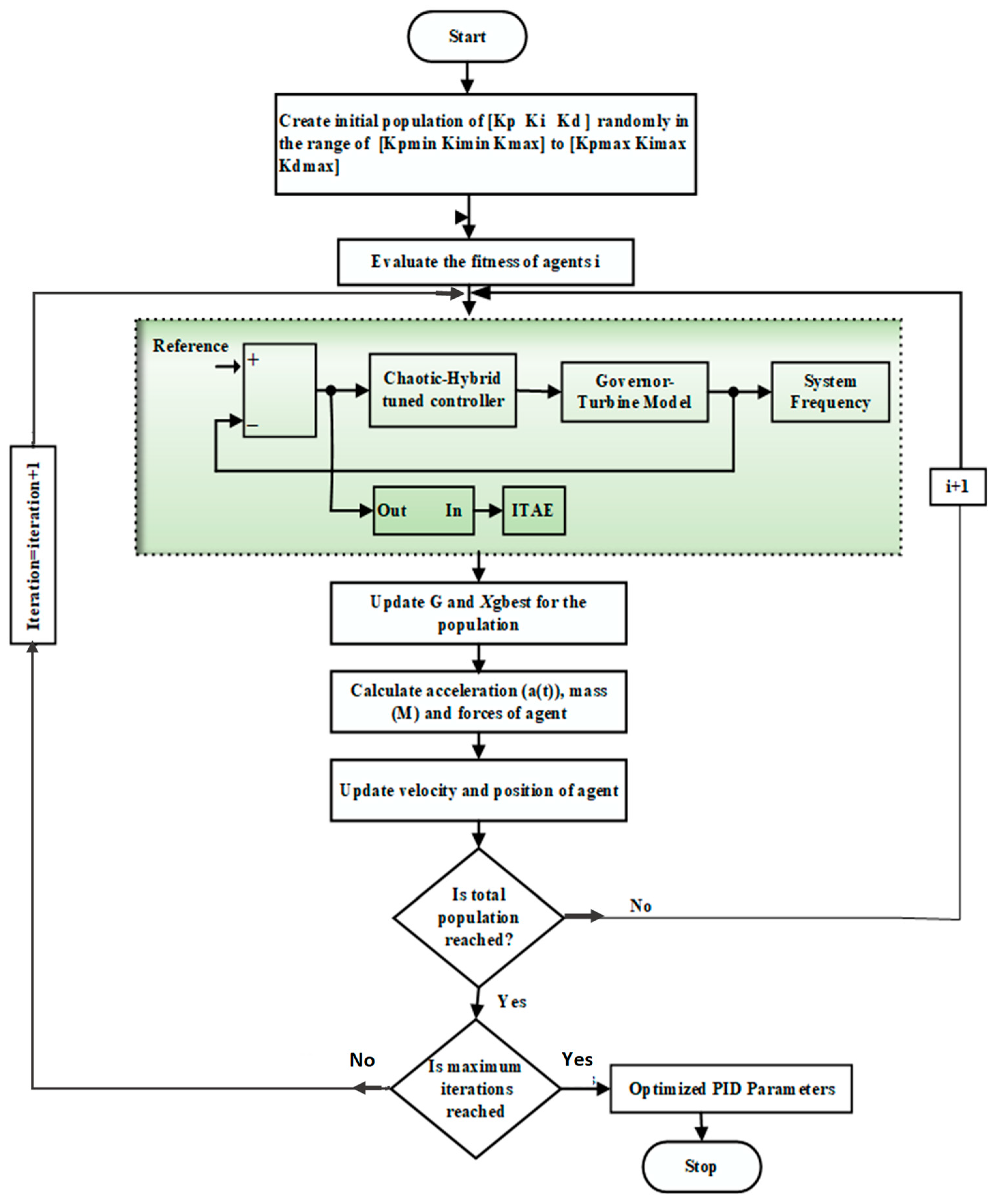
3.1.3. Hybrid SSO-GSA Technique

In meta-heuristic approaches, two techniques can be hybridized at low or high levels, as heterogeneous or homogeneous, with coevolutionary or relay approaches to improve the characteristics of exploration and exploitation to achieve better global minima [40]. In this study, the hybrid SSO-GSA optimization technique is implemented with low-level (merging the functionality of SSO and GSA), co-evolutionary (parallel run of both approaches), and heterogeneous (using two different approaches to get final results) features. The fundamental goal of hybrid SSO-GSA is to combine GSA’s local search capability (aci (t)) with SSO’s social thinking capability (xsgbest). Thus, the integration of both algorithms (SSO and GSA) results in a modified form of velocity Equation (15) expressed as,

$$\begin{array}{c}{\mathrm{V}}_{\mathrm{i}} \left(\mathrm{t}\right)=[\mathrm{D}\times {\mathrm{V}}_{\mathrm{i}} (\mathrm{t})\times {\mathrm{Log}}_{10} (\mathrm{pH}\_{\mathrm{rand}}_1)+\mathrm{rand} \left(\mathrm{n}\right)\times {\mathrm{ac}}_{\mathrm{i}} (\mathrm{t})+{\mathrm{Log}}_{10} (\mathrm{pH}\_{\mathrm{rand}}_2)\\ \times {\mathrm{Log}}_{10} (\mathrm{Temp}\_{\mathrm{rand}}_1)\times ({\mathrm{X}}_{\mathrm{Sgbest}}-{\mathrm{X}}_{\mathrm{i}} (\mathrm{t}\left)\right)]\end{array}$$

(23)

where D is the damping factor of velocity, V_i (t) is the velocity of the agent, pH_rand₁ and pH_rand₂ are the metrics of pH, Temp_rand₁ is the metric of temperature, rand (n) is the random constant (varying between 0 and 1), and ac_i (t) is the acceleration of agent “i” at iteration “t”. X_Sgbest is the sperm global best value, and X_i (t) is the current location of swarm. For this proposed control algorithm, the pH range of 7 to 14 was chosen because it is particularly suited for sperm motility and is regarded as very alkaline and non-toxic to sperm. The temperature inside the vagina ranged from 35.1 to 37.4 degrees Celsius, according to the study of several research works. This temperature can increase to 38.5 degrees Celsius in some cases due to vaginal blood pressure circulation. Based on this information, the temperature range was determined to be between 35.1 and 38.5 degrees Celsius [19,22]

The position of sperm at each iteration is updated as per the following expression:

X_i (t + 1) = X_i (t) + V_i (t + 1)

(24)

The process steps of the hybrid SSO-GSA technique are outlined below:

Step 1: Initialization of all agents randomly; X_i (i = 1, 2, 3,……, N),

Step 2: Evaluate the fitness for all the agents

• Estimate the gravitational force (using Equation (17)),
• Estimate the gravitational constant (using Equation (18)),
• Estimate the resultant forces (using Equation (19)),
• Estimation of acceleration of sperm (using Equation (20)),

Step 3: Update the velocities, V_i (t) (using Equation (23)),

Step 4: Update the positions X_i, (t) (using Equation (24)).

Step 5: Return the best search agent.

3.1.4. Chaotic-Based Hybrid SSO-GSA

In mathematics, chaos can be defined as “randomness,” and it is greatly dependent on the initial conditions of the problem. Small changes in the parameters or beginning values of data in chaotic systems lead to dramatically diverse future behaviors, such as stable fixed points, periodic oscillations, bifurcations, and ergodicity. Furthermore, because of its own periodicity, chaotic motion can pass through each state in a specific region, and each state can only be achieved once [25,41]. Chaos can be used as an alternative to offer the diversity of search during the optimization process. Due to its non-repetition feature, it can be incorporated into the process of metaheuristic algorithms to enhance the convergence rate and avoid being trapped in local minima [42]. To accomplish this, chaotic maps are employed in the process of metaheuristic algorithms for generating chaotic sequences. The 1D chaotic maps are the most extensively used maps due to their simple structure and easy implementation [43]. There are different chaotic maps available, which include the circle map, cubic map, gauss map, iterative chaotic map with infinite collapses (ICMIC), logistic map, sine map, tent map, Chebyshev map, piecewise map, and singer map [34,44]. Among these maps, the sine map is one of the most popular 1D chaotic maps, which is used to enhance the search capability and convergence speed of optimization techniques [43]. Therefore, in this study, a 1D chaotic sine map is implemented with a hybrid SSO-GSA optimization technique to improve the performance of the PID controller in ALFC of HPS. The sine map is a simple 1D chaotic map that generates a chaotic sequence as per the expression of the sine function given below [45]:

$$x_{k+1}=rsin\left(\pi x_k\right)$$

(25)

where the sine function is a function that transforms an input angle into a range of (0, 4), and the sine map exhibits satisfactory chaotic behavior when r $\in$ (0.7, 4).

The process of tuning controller parameters with a chaotic-based hybrid SSO-GSA technique is shown in Figure 5. With consideration of implementing a chaotic function, the modified velocity Equation (23) of the hybrid SSO-GSA optimization algorithm can be expressed as,

$$\begin{array}{c}{\mathrm{V}}_{\mathrm{i}} \left(\mathrm{t}\right)=[\mathrm{Chaos} (\mathrm{n})\times {\mathrm{V}}_{\mathrm{i}} (\mathrm{t})\times {\mathrm{Log}}_{10} (\mathrm{pH}\_{\mathrm{rand}}_1)+\mathrm{Chaos} \left(\mathrm{n}\right)\times {\mathrm{ac}}_{\mathrm{i}} (\mathrm{t})+{\mathrm{Log}}_{10} \\ (\mathrm{pH}\_{\mathrm{rand}}_2)\times {\mathrm{Log}}_{10} (\mathrm{Temp}\_{\mathrm{rand}}_1)\times ({\mathrm{X}}_{\mathrm{Sgbest}}-{\mathrm{X}}_{\mathrm{i}} (\mathrm{t}\left)\right)]\end{array}$$

(26)

where chaos (n) is the sine function given in Equation (25), V_i (t) is the velocity of agent, pH_rand₁ and pH_rand₂ are the metrics of pH (varying between 7 and 14), Temp_rand₁ is the metric of temperature (varying between 35.1 and 38.5 degrees Celsius), and ac_i (t) is the acceleration of agent “i” at iteration “t”. X_Sgbest is the sperm global best value, and X_i (t) is the current location of swarm. SSO (velocity damping factor, D–rand (0, 1), temperature–rand (35.5, 38.5), pH–rand (7, 14), swarm size–30, and total number of iterations–100) are the parameters assumed for tuning the gains of the following: the PID controller, SSO-GSA and CSSO-GSA (velocity damping factor, D–rand (0,1); temperature–rand (35.5, 38.5); pH–rand (7, 14); constant, α = 20; initial gravitational constant, G₀ = 1; total number of agents = 30; and number of iterations = 100). The tuned control gains of the PID controller by the proposed chaotic-based SSO-GSA technique and other techniques (SSO, GSA, and SSO-GSA) for different conditions (Case 1(a): integration of all power sources in HPS; Case 1(b): integration of thermal power and bio energy sources in HPS; Case 1(c): integration of thermal power and RE sources in HPS) are illustrated in

Table 1. Tuned gain parameters of the PID controller with different techniques.

Case Conditions	Control Gains	SSO	GSA	SSO-GSA	Ch SSO-GSA
1(a)	Kp	−9.912	−6.057	−7.00	−6.998
	Ki	−17.00	−15.360	−17.00	−16.999
	Kd	−4.739	−4.145	−3.844	−3.677
1(b)	Kp	−7.822	−6.154	−6.942	−7.00
	Ki	−13.344	−15.230	−16.951	−16.985
	Kd	−2.70	−4.264	−3.409	−2.877
1(c)	Kp	−10.638	−7.821	−6.993	−6.993
	Ki	−16.515	−9.129	−14.458	−16.726
	Kd	−3.207	−3.001	−2.709	−2.702

, as below:

4. Results and Discussion

In this section, the results of time domain analysis for the interconnected two-area HPS model with implementation of the chaotic-based SSO-GSA tuned controller of LFC are described in detail. The HPS model with integration of multiple power sources was developed in a Matlab-Simulink software (R2014b) environment, and the simulation analysis was carried out for various conditions. Among the many power sources, conventional thermal reheat power units with accompanying system non-linearities (GDB) and GRC) are considered the primary power sources in both the areas of power network. In addition, the bioenergy system is considered another important source with the inclusion of bio-diesel and bio-gas generators. In addition, the bioenergy system, which includes bio-diesel and bio-gas generators, is considered another important source. The fuel for the bio-diesel unit is recovered from energy crops via transesterification and has qualities similar to diesel fuel used in traditional diesel engine generators. The bio-gas supply for the bio-gas unit is made from animal waste and biodegradable trash. The bio-gas and bio-diesel power units also consist of a gas valve actuator, combustor, governor, and gas turbine. The RE sources, STPS, and WTGS provide additional power support in the network, and they are not included in the LFC loop because their power output is intermittent and weather dependent. The storage device, which combines AE and FC, is used in tandem to smooth out the power volatility of RE sources.

In order to test the effectiveness of the proffered chaotic-based SSO-GSA controller, the simulation analysis was carried out with various combinations of power sources interconnected to the HPS model. Furthermore, a sensitivity analysis was carried out to validate the robustness of the proffered controller under varying loads and real-time weather intermittency of RE sources.

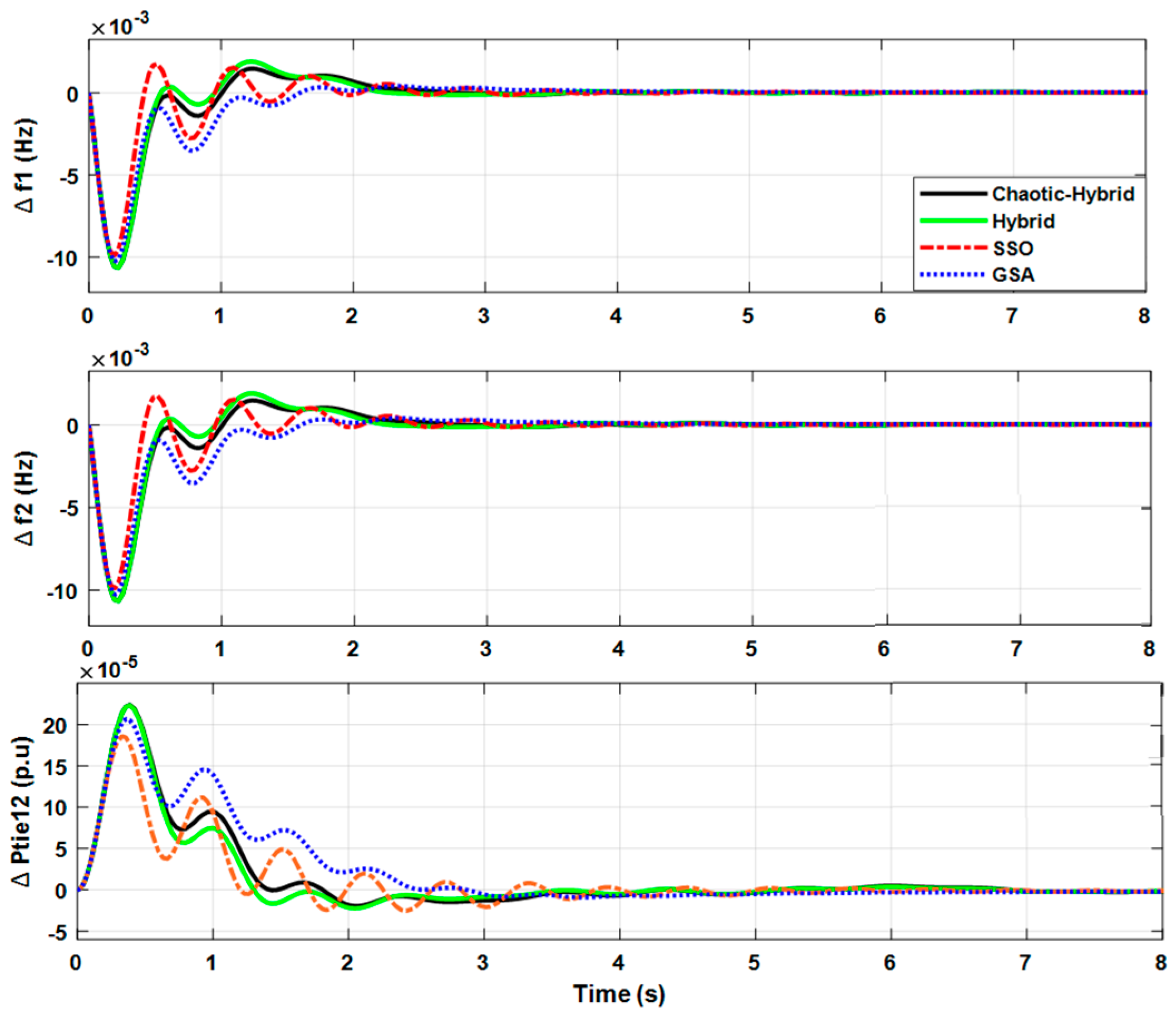
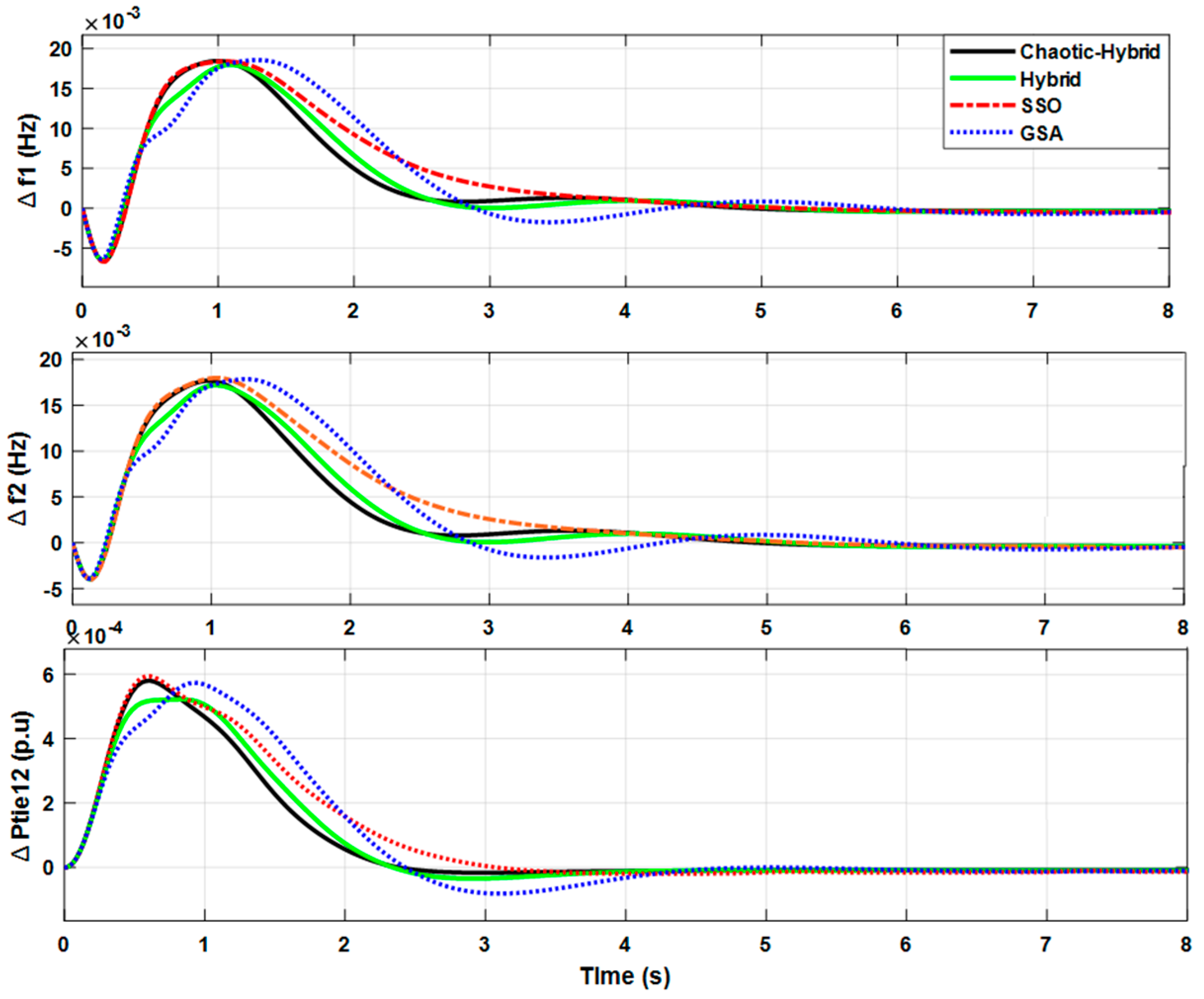
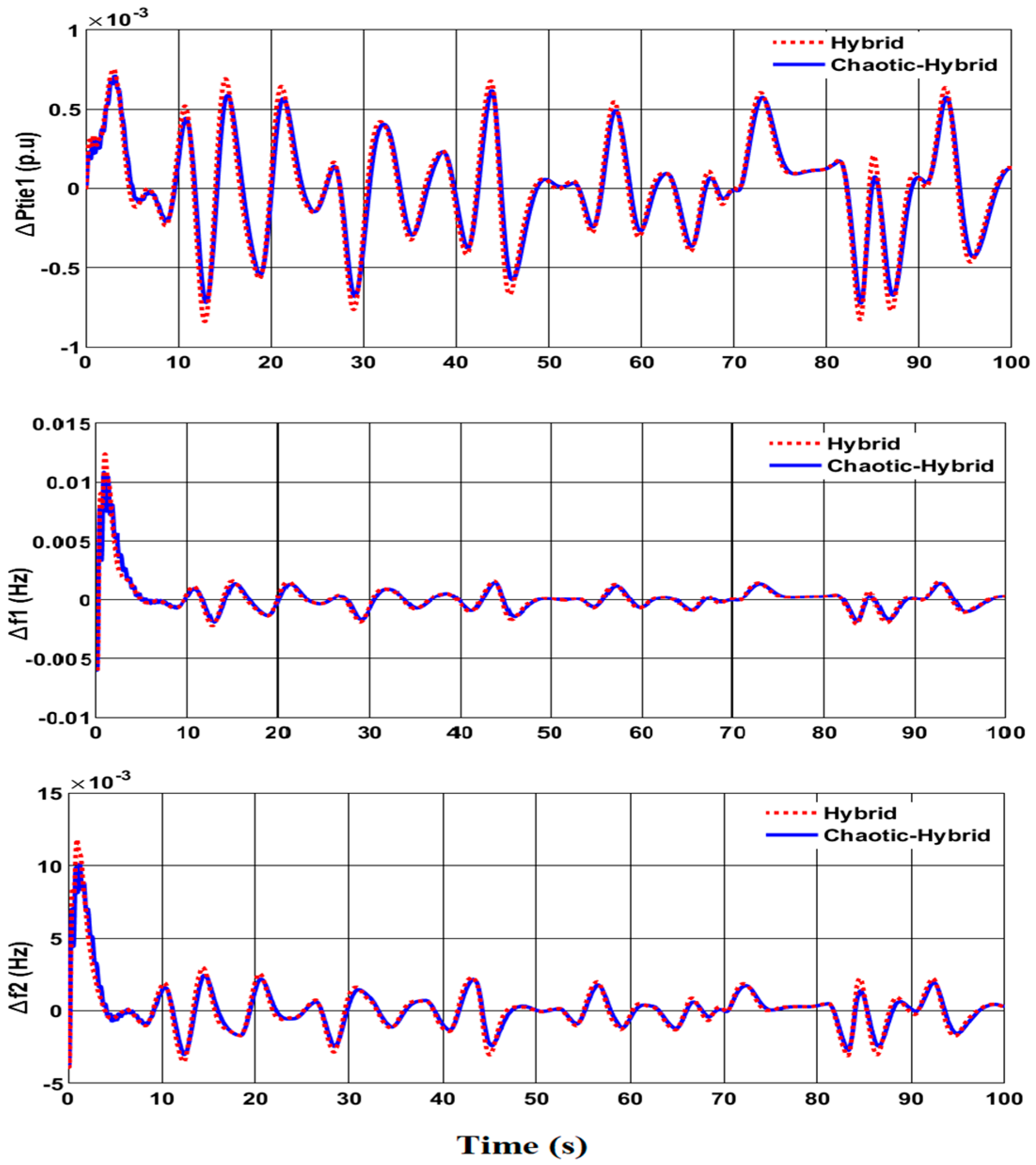
4.1. Time Domain Analysis of HPS with Integration of Different Power Sources

In this case, the analysis was carried out with the integration of different combinations of power sources such as: Case 1(a), all power sources (thermal reheat + bio (bio-gas and bio-diesel) + RE (solar thermal and wind); Case 1(b)), thermal reheat with bio-power sources; and Case 1(c), thermal reheat with RE sources in the HPS model.

Case 1(a): Time domain analysis with integration of all power sources.

In this case, the integration of all generation sources of a reheat thermal power source with non-linearities (GDB of 0.05% and GRC of 3% p.u (MW/min)), bio-energy sources (bio-gas and bio-diesel), and RE sources (solar thermal and wind power) with the inclusion of energy storage systems (AE and FC) was considered in both the areas of HPS with a step load perturbation (SLP) of 0.01 p.u (area 1) and 0.0125 p.u (area 2) of plant capacity (2000 MW). The total power generation from all the power sources of the HPS network can be expressed as:

$$P_{Tg}{=\mathrm{P}}_{\mathrm{Thermal}}{+\mathrm{P}}_{\mathrm{bd} }{+\mathrm{P}}_{\mathrm{bg}}{+\mathrm{P}}_{\mathrm{Wind}}{+\mathrm{P}}_{\mathrm{Solar}}-{\mathrm{P}}_{\mathrm{AE} }{+\mathrm{P}}_{\mathrm{FC}}$$

(27)

The system dynamic responses in terms of frequency deviation and tie-line power variation are shown in Figure 6. The results show that the chaotic-based hybrid tuned PID controller settles into a steady-state faster than the SSO, GSA, and hybrid tuned techniques. The results of steady-state performance indices (integral time absolute error (ITAE), integral absolute error (IAE), integral time square error (ITSE), and integral square error (ISE)), and transient performance indices (control effort (CE), settling time (ST), rise time (RT), and peak magnitude (|P-M|)) of frequency deviations (Δf₁) in area 1, frequency deviations (Δf₂) in area 2, and tie line power variations (ΔP_tie) of HPS, are illustrated in

Table 2. Results of frequency deviation (Δf₁) in area 1 of HPS—Case 1(a).

Case 1(a)	Δf1
	ST (s)	RT (s) ×10−5	|P-M|	IAE ×10−2	ITAE ×10−2	ISE ×10−4	ISTE ×10−4	CE
SSO	8.9611	1.5021	0.0117	1.91	5.87	1.703	1.466	0.4298
GSA	7.3772	1.6212	0.0122	2.229	5.94	1.717	2.062	0.4737
Hybrid	5.0012	1.4721	0.0116	1.908	4.967	1.361	1.492	0.4297
Chaotic-Hybrid	4.9149	1.2282	0.009	1.906	4.961	1.361	1.365	0.4293

,

Table 3. Results of frequency deviation (Δf₂) in area 2 of HPS—Case 1(a).

Case 1(a)	Δf2
	ST (s)	RT (s) ×10−5	|P-M|	IAE ×10−2	ITAE ×10−2	ISE ×10−4	ISTE ×10−4	CE
SSO	7.7883	1.1822	0.0125	2.098	5.727	1.51	1.516	0.4231
GSA	7.3174	1.2758	0.0128	2.011	5.097	1.52	1.526	0.4674
Hybrid	4.9754	1.1583	0.0126	2.011	5.097	1.52	1.52	0.4244
Chaotic-Hybrid	4.9081	1.1469	0.0109	2.007	5.087	1.215	1.465	0.4219

and

Table 4. Results of tie-line power deviation (ΔP_tie) of HPS—Case 1(a).

Case 1(a)	ΔPtie
	ST (s)	RT (s) ×10−5	|P-M| ×10−4	IAE ×10−4	ITAE ×10−3	ISE ×10−7	ISTE ×10−7	CE
SSO	7.6649	0.1035	3.926	5.695	2.145	1.4	1.201	0.0117
GSA	4.9898	0.1208	4.1778	6.724	1.619	1.66	1.69	0.0131
Hybrid	3.9631	0.1059	3.8427	5.588	1.245	1.31	1.19	0.0119
Chaotic-Hybrid	3.8716	0.1034	3.8235	5.643	1.237	1.31	1.17	0.0112

, respectively. From the results of the Case 1(a) analysis, it is inferred that the steady-state performance indices were substantially improved with the chaotic-based hybrid tuned controller than with other techniques (hybrid, SSO, and GSA). Furthermore, the tie-line power tends to be more stable and smooth with the proffered chaotic-based hybrid strategy than other methods. In addition, the results of transient indices show that the proffered method (chaotic hybrid) exhibits minimal ST (s) with a reduced CE, RT, and |P-M| than other methods (hybrid, SSO, and GSA).

Case 1(b): Time domain analysis with integration of thermal power and bio energy sources

In this case, the system consits of bio-diesel and bio-gas units along with a thermal reheat power source in each area of the interconnected HPS model with SLP as specified in Case 1(a). The total power generation can be expressed as,

$$P_{Tg}{=\mathrm{P}}_{\mathrm{Thermal}}{+\mathrm{P}}_{\mathrm{bd} }{+\mathrm{P}}_{bg}$$

(28)

The dynamic response of frequency and tie-line power variations of the HPS model for Case 1(b) is shown in Figure 7. The steady-state and transient performance indices recorded are illustrated in

Table 5. Results of frequency deviation (Δf₁) in area 1 of HPS—Case 1(b).

Case 1(b)	Δf1
	ST (s)	RT (s) ×10−5	|P-M|	IAE ×10−2	ITAE ×10−2	ISE ×10−4	ISTE ×10−4	CE
SSO	11.8398	1.7903	0.018	3.714	12.09	3.894	4.911	0.7275
GSA	11.1111	1.907	0.0179	3.556	11.05	3.88	5.201	0.6362
HSSO-GSA	10.0584	1.4721	0.0116	2.966	9.047	3.071	3.565	0.5712
Chaotic-Hybrid	9.7448	1.2282	0.0115	2.951	9.006	3.069	3.371	0.57

,

Table 6. Results of frequency deviation (Δf₂) in area 2 of HPS—Case 1(b).

Case 1(b)	Δf2
	ST (s)	RT (s) ×10−5	|P-M|	IAE ×10−2	ITAE ×10−2	ISE ×10−4	ISTE ×10−4	CE
SSO	11.7259	1.7495	0.0184	3.862	12.35	4.207	5.363	0.721
GSA	10.9367	1.5025	0.0185	3.697	11.37	4.172	5.746	0.6306
Hybrid	9.7646	1.3517	0.0185	3.098	9.254	3.343	3.963	0.5652
Chaotic-Hybrid	9.2949	1.3488	0.0184	3.017	9.225	3.323	3.768	0.5636

and

Table 7. Results of tie-line power deviation (ΔP_tie) of HPS—Case 1(b).

Case 1(b)	ΔPtie
	ST (s)	RT (s) ×10−5	|P-M| ×10−4	IAE ×10−4	ITAE ×10−3	ISE ×10−7	ISTE ×10−7	CE
SSO	8.7086	10.88	5.938	9.416	2.639	3.355	3.211	0.0185
GSA	7.4632	9.3586	5.7349	10.07	2.724	3.505	3.788	0.0171
Hybrid	4.2268	0.295	5.2203	8.294	2.209	2.769	2.531	0.0156
Chaotic-Hybrid	3.8279	0.2947	3.8235	7.823	2.109	2.724	2.292	0.0154

, respectively. The results show that the range of deviations in frequency and tie-line power level was increased as compared to previous case analysis of 1(a), due to the absence of RE power generation and storage devices. However, the steady-state indices were significantly improved with the chaotic-based hybrid tuned PID controller than with other methods (SSO, GSA, and hybrid). Furthermore, the proposed controller (chaotic-hybrid) outperforms the other methods presented in terms of minimum ST and reduced CE, RT, and |P-M| than other methods presented.

Case 1(c): Time domain analysis with integration of thermal power and RE sources.

The thermal reheat power source with integration of RE sources (solar thermal, wind power) and storage devices (AE and FC) was considered in this case of the HPS model with SLP as discussed in Case 1(a). The total power generation of connected power sources can be expressed as,

$$P_{Tg}{=\mathrm{P}}_{\mathrm{Thermal}}{+\mathrm{P}}_{\mathrm{Wind}}{+\mathrm{P}}_{\mathrm{Solar}}-{\mathrm{P}}_{\mathrm{AE}}{+\mathrm{P}}_{\mathrm{FC}}$$

(29)

The dynamic response of frequency and tie-line power variations is shown in Figure 8. The performance indices of the steady-state and transient state are illustrated in

Table 8. Results of frequency deviation (Δf₁) in area 1 of HPS—Case 1(c).

Case 1(c)	Δf1
	ST (s)	RT (s) ×10−5	|P-M|	IAE ×10−3	ITAE ×10−2	ISE ×10−5	ISTE ×10−6	CE
SSO	3.2277	1.1733	0.0079	4.582	6.411	2.12	6.93	0.0765
GSA	3.4342	1.2096	0.0082	5.579	7.41	2.64	8.18	0.1096
Hybrid	2.4341	1.79	0.0086	4.949	2.69	2.04	6.55	0.074
Chaotic-Hybrid	2.2529	1.006	0.0086	4.357	2.587	2.03	5.96	0.065

,

Table 9. Results of frequency deviation (Δf₂) in area 2 of HPS—Case 1(c).

Case 1(c)	Δf2
	ST (s)	RT (s) ×10−6	|P-M|	IAE ×10−3	ITAE ×10−2	ISE ×10−5	ISTE ×10−6	CE
SSO	2.9461	2.4659	0.0109	4.582	6.411	2.82	8.93	0.0768
GSA	3.1682	3.6062	0.0108	5.579	7.041	2.64	8.58	0.1124
Hybrid	2.4166	4.6685	0.0106	4.9403	2.638	2.78	8.52	0.0767
Chaotic-Hybrid	2.1222	1.4119	0.0106	4.4899	2.627	2.79	8.48	0.0682

and

Table 10. Results of tie-line power deviation (ΔP_tie) of HPS—Case 1(c).

Case 1(c)	ΔPtie
	ST (s)	RT (s) ×10−4	|P-M| ×10−4	IAE ×10−4	ITAE ×10−4	ISE ×10−8	ISTE ×10−8	CE
SSO	6.0225	1.4713	0.3852	3.59	3.37	1.93	7.91	0.0026
GSA	5.9878	1.88883	0.3852	2.33	5.69	2.37	0.67	0.0047
Hybrid	3.3736	1.46258	0.3827	2.32	2.895	1.80	1.88	0.0032
Chaotic-Hybrid	2.8889	1.226	0.3827	2.3	2.595	1.6	4.91	0.0024

, respectively. The results show that the oscillations in frequency were reduced as compared to Cases 1(a) and 1(b), respectively. The integration of RE sources with energy storage supports the real power exchange without any abbreations, which improves the frequency regulation of the system. The proposed method of chaotic-hybrid shows superior performance in terms of steady-state (IAE, ITAE, ISE and ITSE) and transient (ST, RT and |P-M|) performance indices, and control effort of the controller than other tuning techniques. This is achieved through improved search ability of a hybrid technique with a chaos embedded function. Despite the exceptional performance of the proposed chaotic-hybrid algorithm, chaotic maps have several limitations while used with meta-heuristic algorithms. That is, there is the need for a large number of experiments during the design phase in order to choose the right type of maps for the problem to be solved. Future studies could broaden the scope of this paper by examining the use of various chaotic maps and comparing the performance of single and multiple chaotic maps in local search.

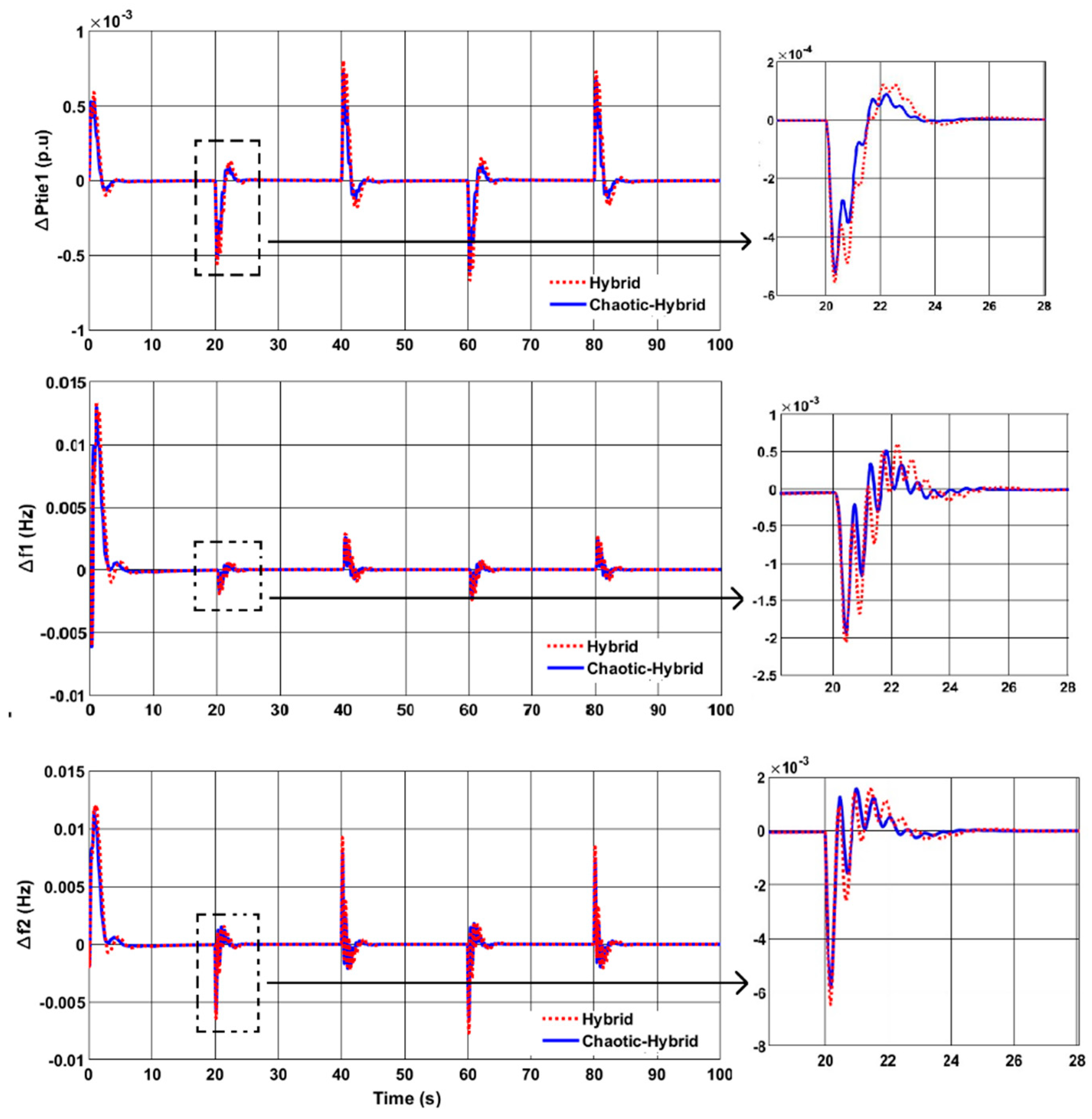
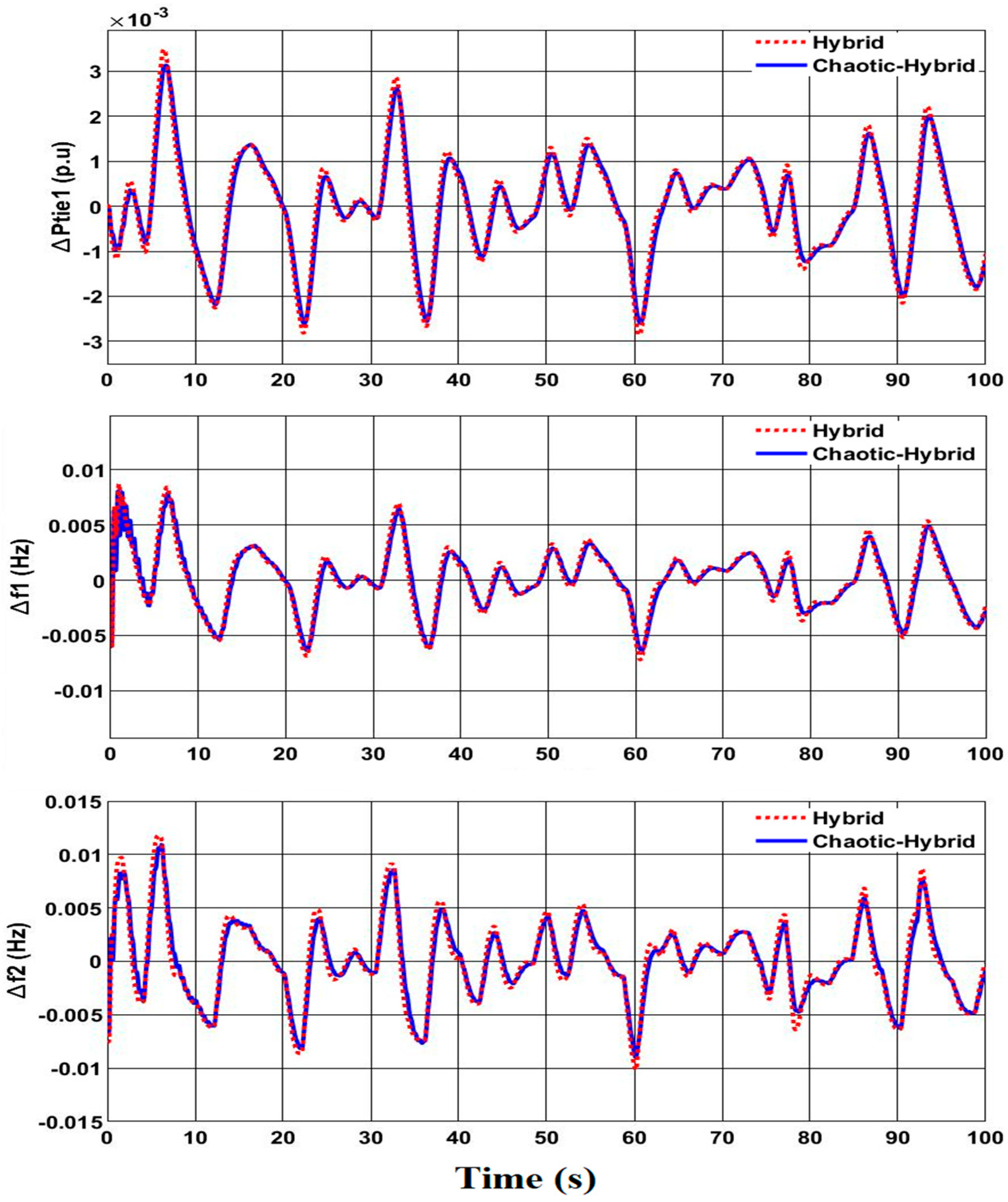
4.2. Sensitivity Analysis

The robustness of the chaotic-hybrid tuned PID controller was verified by examining its performance under various conditions (load variation, real time solar, and wind power variation) of the HPS model. The system model considered for analysis is the same as Case 1(a). First, the proposed controller’s adaptiveness was validated with a random change load profile, as shown in Figure 9. The load demand was changing with consecutive load perturbations of 0.007, 0.015, 0.003, 0.0125, and 0.002 p.u. of plant capacity in area 1 at time intervals of 0, 20, 40, 60, and 80 s, while area 2 remained constant at 0.0125 p.u. The deviations in frequency (Δf₁ and Δf₂) and tie-line power (ΔP_tie) of the interconnected HPS network for these uncertain load changes are shown in the Figure 10. From the results, it is inferred that the deviations in frequency and tie-line power were settled faster with the proposed chaotic-hybrid method of tuning the controller. As per the load profile (Figure 9), when there is an increment of load (at 20 s), the results of power deviation (ΔP_tie) as shown in Figure 10 clearly indicate that the proposed chaotic-hybrid method offers reduced power devaition (ΔP_tie = −5.24 × 10⁻⁴ p.u) than with the hybrid method (ΔP_tie = −5.58 × 10⁻⁴ p.u). At same time, reduced frequency deviations in area 1 and 2 (Δf₁ = −1.86 × 10⁻³ Hz and Δf₂ = −5.55 × 10⁻³ Hz) were observed with the proposed chaotic-hybrid method rather than with hybrid control method (Δf₁ = −1.99 × 10⁻³ Hz and Δf₂ = −6.29 × 10⁻³ Hz). When there is a decrement of load (at 40 s), reduced power deviation (ΔP_tie = 7.21 × 10⁻⁴ p.u) and frequency deviations (Δf₁ = 2.63 × 10⁻³ Hz and Δf₂ = 7.97 × 10⁻³ Hz) were observed with the chaotic-hybrid method rather than the power deviation (ΔP_tie = 8.03 × 10⁻⁴ p.u) and frequency deviations (Δf₁ = 2.91 × 10⁻³ Hz and Δf₂ = 9.25 × 10⁻³ Hz) of the hybrid control method. Thus, the proposed technique had a more robust and faster response time to converge into a steady-state under consecutive load disturbances in HPS.

Further, the dynmic response of the proposed technique was verified with the effect of real time solar power variation of STPS (Figure 11) in the HPS network. To study this, real-time solar irradiance data (200 slots with an interval of 0.5 s) from the Subang meterological center of Malaysia [46] was considered. During this case of analysis, the observed dynamic response of frequency and tie-line power deviation are shown in Figure 12. As an example, at 13 s of simultion time (where higher deviations in power and frequency), reduced power deviation (ΔP_tie = −7.18 × 10⁻⁴ p.u) and frequency deviations (Δf₁ = −1.93 × 10⁻³ Hz and Δf₂ = −3.02 × 10⁻³ Hz) were observed with the chaotic-hybrid method rather than with power deviation (ΔP_tie = −8.40 × 10⁻⁴ p.u) and frequency deviations (Δf₁ = −2.27 × 10⁻³ Hz and Δf₂ = −3.52 × 10⁻³ Hz) of the hybrid control method. Thus, from the results, it is seen that the proposed technique provides a better and smoother response with reduced undershoot and overshoot than in the hybrid technique, during the case of real time solar power variation.

Similarly, the effectiveness of the proposed controller was varified with the effect of wind power variation of WTGS (Figure 13). For analysis, the real-time varying wind speed data (200 slots with an interval of 1 s) from the Kuala Terengganu meterological center of Malaysia [47] was considered. The dynamic response of frequency and tie line power deviations of HPS during the case of wind power variation is shown in Figure 14. At simulation time of 6.6 s (where higher deviations in power and frequency), the power deviation (ΔP_tie = 3.12 × 10⁻³ p.u) and frequency deviations (Δf₁ = 7.85 × 10⁻³ Hz and Δf₂ = 10.95 × 10⁻³ Hz) with the chaotic-hybrid method were found to be lesser than power (ΔP_tie = 3.48 × 10⁻³ p.u) and frequency deviations (Δf₁ = 8.44 × 10⁻³ Hz and Δf₂ = 11.57 × 10⁻³ Hz) of the hybrid method. Thus, from the results of varying wind power analysis, it is inferred that the proposed method offers reduced frequency oscillations and steady-state error, as compared to the hybrid method.

Hence, from the results of the sensitivity analysis, it can be concluded that the proposed control method outperforms the hybrid method in terms of controlling frequency and power oscillations during the case of consecutive load disturbances and varying wind/solar power in real time conditions.

4.3. Convergence Performance

The convergence performance of various control techniques (SSO, GSA, hybrid, and chaotic-hybrid) obtained while tuning the gain parameters of the PID controller in the HPS model is discussed in this section. Figure 15 represents the minimization of steady-state performance indices of the ITAE objective function as defined in Equation (11). Based on the fitness curves, it is concluded that the proposed chaotic-based hybrid SSO-GSA method converges faster and performs better than other methods presented. Because of diversification of chaotic sequences in the sine map used, premature convergence was avoided. As a result, the implementation of chaotic sequences in hybrid techniques enhances the exploration and exploitation capability significantly.

4.4. Stability Analysis

A stability analysis was performed to explore the frequency stability for the single area power network of the HPS model with the MSSO tuned controller of the LFC system, as considered in Case 1A. Because the networks in both areas have the same configuration, analyzing stability using a single area power network is sufficient. The order (max. 33) of the closed loop transfer function (CLTF) obtained for the network is higher, and it is difficult to analyze stability for the higher-order system. Therefore, the higher-order transfer function was reduced into a second-order transfer function by the Hankel matrix method. The entire process for model order reduction utilizing the Hankel approach for HPS is given in the authors’ prior study [36]. By applying the Hankel method, the reduced lower-order transfer function of the HPS model was obtained as follows:

$$\mathrm{CLTF}=\frac{-2.104\times {10}^{-9} s+3.565\times {10}^{-11}}{s^2+0.03388 s+0.000287}$$

(30)

The frequency response of the Bode plot for the HPS model is shown in Figure 16, with a gain margin of 144 dB and a gain cross over frequency of 0.0293 (rad/s). The bode analysis response demonstrates that the closed-loop system for the proposed MSSO tuned PID controller of the LFC is stable.

The stability of the closed-loop system was verified in a further level using the second-order Lyapunov method of stability. For analysis, the area control error of interconnected HPS was considered and defined as a positive definite squared error function of the Lyapunov function, expressed as below [11]:

$$E (k_P, k_i, k_d)=\frac{1}{2} e {\left(t\right)}^2$$

(31)

$$E (k_P, k_i, k_d)=\frac{1}{2} e {\left(f_{ref}-f_P\right)}^2$$

(32)

where f_ref is the plant output reference and f_P is the actual plant output.

For the system to be stable, the gradients of Equation (32) should be less than zero and that can be defined as:

$$\frac{dE}{dt}=-\frac{\partial E}{\partial t}$$

(33)

The expression (33) clearly shows that the proposed Lyapunov function is always less than zero, i.e., negative definite (dE/dt ≤ 0). The system cannot persist in a non-equilibrium state in which the energy profile increases monotonically, and it decreases to zero over time or to some constant value to achieve the equilibrium state of the system. This demonstrates the notion of Lyapunov stability [11]. The decrease in energy function profile against time with the proposed controller was observed and presented in Figure 17 to assure the overall system’s stability. As a result, the proposed controller’s energy profile reaches zero and converges the system steady-state error in a deterministic manner by travelling in a negative gradient direction, ensuring the system’s stability in a Lyapunov sense. The system is depicted as behaving in a Lyapunov sense and reaching a stable equilibrium point.

4.5. Comparative Analysis

This section presents a comparative analysis of the proposed technique with different meta-heuristic algorithms (PSO, GWO, SSO, and MFO) used to tune PID controllers in the literature. To study this, a two-area interconnected HPS model as discussed in Case 1(a) has been considered for analysis. The dynamic response of controllers in terms of frequency deviations (Δf₁ and Δf₂) and tie-line power variation (Δp_tie) of the HPS model is portrayed in Figure 18. It is seen from the response that the proposed method quickly settles to a steady-state compared to the PSO, WHO, MFO, and SSO method of tuning the controller. Further, the controller technique has been examined in terms of % improvement in ST and ITAE, as given in

Table 11. Results of comparative analysis.

Optimization Method	Signal	ST (s)	Improved (%) in ST	ITAE (×10−2)	Improved (%) in ITAE
PSO	Δf1	12.3503	-	8.276	-
	Δf2	11.6461	-	8.453	-
WHO	Δf1	8.4912	31.247	5.494	33.615
	Δf2	4.7195	59.476	5.626	33.443
MFO	Δf1	8.625	30.163	5.475	33.844
	Δf2	4.7481	59.23	5.601	33.739
SSO	Δf1	8.9611	27.442	5.87	29.072
	Δf2	7.7883	33.125	5.727	32.248
Chaotic-Hybrid	Δf1	4.9149	60.204	4.961	40.055
	Δf2	4.9081	57.856	5.087	39.820

. It is seen that the proffered chaotic-hybrid method outperforms significantly compared to other techniques presented.

5. Conclusions

In this research work, chaotic-based hybrid SSO-GSA tuned gain parameters of a PID controller are proposed for ALFC application of a two-area-interconnected HPS model. The proffered method is implemented with a 1D chaotic sine map to enhance the search capability and convergence speed of the hybrid (SSO-GSA) optimization method. The performance is examined with other optimization methods (SSO, GSA, and hybrid SSO-GSA) in terms of steady-state (ITSE, IAE, ITSE, and ISE) and transient state indices (ST, RT, and |P-M|), as well as CE of frequency deviations (Δf₁ and Δf₂) and tie-line power variation (ΔP_tie) under differnet conditions (1(a), 1(b), and 1(c)). From the results of case studies, it can be concluded that the profferred chaotic-hybrid tuned PID controller offers excellent performance in terms of enhancing the steady-state indices and minimizing the indices of ST, CE, RT, and |P-M|. Furthermore, a sensitivity analysis was carried out to validate the self adaptiveness and robustness of the proposed controller under various conditions such as load variation and uncertain conditions of wind and solar power sources. From the results of sensitivity analysis, it is inferred that the proposed chaotic-hybrid tuned PID controller outperforms the hybrid technique in terms of controlling frequency and power oscillations during the case of consecutive load disturbances and varying wind/solar power in real time conditions. Moreover, from the analysis of convergence performance, it can be seen that the proposed technique offers excellent performance, as it converges faster than the other algorithms (SSO, GSA, and hybrid SSO-GSA). In addition, results from the stability and comparative analysis clearly indicate that the proposed controller is more stable and exhibits minimum ST and ITAE in terms of frequency deviations than other methods. When compared to the existing control approach, the proposed control strategy achieves a significant improvement in ST and IATE by 60.204% and 40.055% in area 1 and 57.856% and 39.820% in area 2 of frequency control. The development of an improved hybrid control mechanism for optimizing frequency and voltage regulation in multi-area power systems is the future scope of this research endeavor.

References

1. Tungadio, D.H.; Sun, Y. Load frequency controllers considering renewable energy integration in power system. Energy Rep. 2019, 5, 436–453. [Google Scholar] [CrossRef]
2. Arya, Y. AGC performance enrichment of multi-source hydrothermal gas power systems using new optimized FOFPID controller and redox flow batteries. Energy 2017, 127, 704–715. [Google Scholar] [CrossRef]
3. Dash, P.; Saikia, L.C.; Sinha, N. Automatic generation control of multi area thermal system using Bat algorithm optimized PD–PID cascade controller. Int. J. Electr. Power Energy Syst. 2015, 68, 364–372. [Google Scholar] [CrossRef]
4. Mokhtar, M.; Marei, M.I.; Sameh, M.A.; Attia, M.A. An Adaptive Load Frequency Control for Power Systems with Renewable Energy Sources. Energies 2022, 15, 573. [Google Scholar] [CrossRef]
5. Dash, P.; Saikia, L.C.; Sinha, N. Flower Pollination Algorithm Optimized PI-PD Cascade Controller in Automatic Generation Control of a Multi-area Power System. Int. J. Electr. Power Energy Syst. 2016, 82, 19–28. [Google Scholar] [CrossRef]
6. Hamodat, Z.; Cansever, G. Automated Generation Control of Multiple-Area Electrical System with an Availability-Based Tariff Pricing Scheme Regulated by Whale Optimized Fuzzy PID Controller. Int. J. Photoenergy 2021, 2021, 5596527. [Google Scholar] [CrossRef]
7. Gbadega, P.A.; Akindeji, K.T. Linear Quadratic Regulator Technique for Optimal Load Frequency Controller Design of Interconnected Linear Power Systems. In Proceedings of the 2020 IEEE PES/IAS PowerAfrica, Nairobi, Kenya, 25–28 August 2020. [Google Scholar]
8. Sun, Y.; Wang, Y.; Wei, Z.; Sun, G.; Wu, X. Robust H load frequency control of multi-area power system with time delay: A sliding mode control approach. IEEE/CAA J. Autom. Sin. 2017, 5, 610–617. [Google Scholar] [CrossRef]
9. Fathy, A.; Kassem, A.M.; Abdelaziz, A.Y. Optimal design of fuzzy PID controller for deregulated LFC of multi-area power system via mine blast algorithm. Neural Comput. Appl. 2018, 32, 4531–4551. [Google Scholar] [CrossRef]
10. Rizwan, R.; Arshad, J.; Almogren, A.; Jaffery, M.H.; Yousaf, A.; Khan, A.; Rehman, A.U.; Shafiq, M. Implementation of ANN-Based Embedded Hybrid Power Filter Using HIL-Topology with Real-Time Data Visualization through Node-RED. Energies 2021, 14, 7127. [Google Scholar] [CrossRef]
11. Ramachandran, R.; Madasamy, B.; Veerasamy, V.; Saravanan, L. Load frequency control of a dynamic interconnected power system using generalised Hopfield neural network based self-adaptive PID controller. IET Gener. Transm. Distrib. 2018, 12, 5713–5722. [Google Scholar] [CrossRef]
12. Weldcherkos, T.; Salau, A.O.; Ashagrie, A. Modeling and design of an automatic generation control for hydropower plants using Neuro-Fuzzy controller. Energy Rep. 2021, 7, 6626–6637. [Google Scholar] [CrossRef]
13. Sarwar, S.; Javed, M.Y.; Jaffery, M.H.; Arshad, J.; Rehman, A.U.; Shafiq, M.; Choi, J.-G. A Novel Hybrid MPPT Technique to Maximize Power Harvesting from PV System under Partial and Complex Partial Shading. Appl. Sci. 2022, 12, 587. [Google Scholar] [CrossRef]
14. Gheisarnejad, M. An effective hybrid harmony search and cuckoo optimization algorithm based fuzzy PID controller for load frequency control. Appl. Soft Comput. 2018, 65, 121–138. [Google Scholar] [CrossRef]
15. Veerasamy, V.; Wahab, N.I.A.; Ramachandran, R.; Vinayagam, A.; Othman, M.L.; Hizam, H.; Satheeshkumar, J. Automatic Load Frequency Control of a Multi-Area Dynamic Interconnected Power System Using a Hybrid PSO-GSA-Tuned PID Controller. Sustainability 2019, 11, 6908. [Google Scholar] [CrossRef] [Green Version]
16. Khadanga, R.K.; Kumar, A. Analysis of PID controller for the load frequency control of static synchronous series compensator and capacitive energy storage source-based multi-area multi-source interconnected power system with HVDC link. Int. J. Bio-Inspired Comput. 2019, 13, 131–139. [Google Scholar] [CrossRef]
17. Duman, S.; Yorukeren, N.; Altas, I.H. A novel modified hybrid PSOGSA based on fuzzy logic for non-convex economic dispatch problem with valve-point effect. Int. J. Electr. Power Energy Syst. 2015, 64, 121–135. [Google Scholar] [CrossRef]
18. Shehadeh, H.A.; Ahmedy, I.; Idris, M.Y.I. Sperm swarm optimization algorithm for optimizing wireless sensor network challenges. In Proceedings of the 6th International Conference on Communications and Broadband Networking, Singapore, 24–26 February 2018. [Google Scholar]
19. Shehadeh, H.A.; Ahmedy, I.; Idris, M.Y.I. Empirical Study of Sperm Swarm Optimization Algorithm. In Intelligent Systems and Applications, Proceedings of the SAI Intelligent Systems Conference, London, UK, 6–7 September 2018; Springer: Cham, Switzerland, 2019. [Google Scholar]
20. Mittal, H.; Tripathi, A.; Pandey, A.C.; Pal, R. Gravitational search algorithm: A comprehensive analysis of recent variants. Multimedia Tools Appl. 2020, 80, 7581–7608. [Google Scholar] [CrossRef]
21. Shehadeh, H.A.; Idris, M.Y.I.; Ahmedy, I.; Ramli, R.; Noor, N.M. The Multi-Objective Optimization Algorithm Based on Sperm Fertilization Procedure (MOSFP) Method for Solving Wireless Sensor Networks Optimization Problems in Smart Grid Applications. Energies 2018, 11, 97. [Google Scholar] [CrossRef] [Green Version]
22. Shehadeh, H.A.; Ldris, M.Y.I.; Ahmedy, I. Multi-Objective Optimization Algorithm Based on Sperm Fertilization Procedure (MOSFP). Symmetry 2017, 9, 241. [Google Scholar] [CrossRef]
23. Ghorbani, M.A.; Deo, R.C.; Karimi, V.; Kashani, M.H.; Ghorbani, S. Design and implementation of a hybrid MLP-GSA model with multi-layer perceptron-gravitational search algorithm for monthly lake water level forecasting. Stoch. Environ. Res. Risk Assess. 2018, 33, 125–147. [Google Scholar] [CrossRef]
24. Khokhar, B.; Dahiya, S.; Parmar, K.S. Load frequency control of a microgrid employing a 2D Sine Logistic map based chaotic sine cosine algorithm. Appl. Soft Comput. 2021, 109, 107564. [Google Scholar] [CrossRef]
25. Chen, F.; Tang, B.; Song, T.; Li, L. Multi-fault diagnosis study on roller bearing based on multi-kernel support vector machine with chaotic particle swarm optimization. Measurement 2014, 47, 576–590. [Google Scholar] [CrossRef]
26. Mokeddem, D. A new improved salp swarm algorithm using logarithmic spiral mechanism enhanced with chaos for global optimization. Evol. Intell. 2021, 14, 1–31. [Google Scholar] [CrossRef]
27. Sayed, G.I.; Hassanien, A.E.; Azar, A.T. Feature selection via a novel chaotic crow search algorithm. Neural Comput. Appl. 2017, 31, 171–188. [Google Scholar] [CrossRef]
28. Sayed, G.I.; Khoriba, G.; Haggag, M.H. A novel chaotic salp swarm algorithm for global optimization and feature selection. Appl. Intell. 2018, 48, 3462–3481. [Google Scholar] [CrossRef]
29. Kohli, M.; Arora, S. Chaotic grey wolf optimization algorithm for constrained optimization problems. J. Comput. Des. Eng. 2018, 5, 458–472. [Google Scholar] [CrossRef]
30. Poojitha, S.N.; Jothiprakash, V.; Sivakumar, B. Chaos-directed genetic algorithms for water distribution network design: An enhanced search method. Stoch. Environ. Res. Risk Assess. 2022, 28, 1–17. [Google Scholar] [CrossRef]
31. Arora, S.; Anand, P. Chaotic grasshopper optimization algorithm for global optimization. Neural Comput. Appl. 2018, 31, 4385–4405. [Google Scholar] [CrossRef]
32. Xu, G.-H.; Zhang, T.-W.; Lai, Q. A new firefly algorithm with mean condition partial attraction. Appl. Intell. 2021, 52, 4418–4431. [Google Scholar] [CrossRef]
33. Yi, J.; Huang, J.; Zhou, W.; Chen, G.; Zhao, M. Intergroup Cascade Broad Learning System with Optimized Parameters for Chaotic Time Series Prediction. IEEE Trans. Artif. Intell. 2022, 53, 1–7. [Google Scholar] [CrossRef]
34. Das, S.; Saha, P. Performance of swarm intelligence based chaotic meta-heuristic algorithms in civil structural health monitoring. Measurement 2020, 169, 108533. [Google Scholar] [CrossRef]
35. Das, D.C.; Roy, A.K.; Sinha, N. GA based frequency controller for solar thermal–diesel–wind hybrid energy generation/energy storage system. Int. J. Electr. Power Energy Syst. 2012, 43, 262–279. [Google Scholar] [CrossRef]
36. Veerasamy, V.; Wahab, N.I.A.; Ramachandran, R.; Othman, M.L.; Hizam, H.; Irudayaraj, A.X.R.; Guerrero, J.M.; Kumar, J.S. A Hankel Matrix Based Reduced Order Model for Stability Analysis of Hybrid Power System Using PSO-GSA Optimized Cascade PI-PD Controller for Automatic Load Frequency Control. IEEE Access 2020, 8, 71422–71446. [Google Scholar] [CrossRef]
37. Barik, A.K.; Das, D.C. Expeditious frequency control of solar photovoltaic/biogas/biodiesel generator based isolated renewable microgrid using grasshopper optimisation algorithm. IET Renew. Power Gener. 2018, 12, 1659–1667. [Google Scholar] [CrossRef]
38. Farahani, M.; Ganjefar, S.; Alizadeh, M. PID controller adjustment using chaotic optimisation algorithm for multi-area load frequency control. IET Control Theory Appl. 2012, 6, 1984–1992. [Google Scholar] [CrossRef]
39. Shehadeh, H.A. A hybrid sperm swarm optimization and gravitational search algorithm (HSSOGSA) for global optimization. Neural Comput. Appl. 2021, 33, 11739–11752. [Google Scholar] [CrossRef]
40. Talbi, E.-G. A Taxonomy of Hybrid Metaheuristics. J. Heuristics 2002, 8, 541–564. [Google Scholar] [CrossRef]
41. Tang, R.; Fong, S.; Dey, N. Metaheuristics and Chaos Theory. In Chaos Theory; InTech: Rijeka, Croatia, 2018; pp. 182–196. [Google Scholar]
42. dos Santos Coelho, L. Tuning of PID controller for an automatic regulator voltage system using chaotic optimization approach. Chaos Solitons Fractals 2009, 39, 1504–1514. [Google Scholar] [CrossRef]
43. Demir, F.B.; Tuncer, T.; Kocamaz, A.F. A chaotic optimization method based on logistic-sine map for numerical function optimization. Neural Comput. Appl. 2020, 32, 14227–14239. [Google Scholar] [CrossRef]
44. Kaveh, A. Advances in Metaheuristic Algorithms for Optimal Design of Structures; Springer: Cham, Switzerland, 2014. [Google Scholar]
45. Zhou, Y.; Bao, L.; Chen, C.L.P. A new 1D chaotic system for image encryption. Signal Process. 2014, 97, 172–182. [Google Scholar] [CrossRef]
46. Lurwan, S.M.; Mariun, N.; Hizam, H.; Radzi, M.A.M.; Zakaria, A. Predicting power output of photovoltaic systems with solar radiation model. In Proceedings of the 2014 IEEE International Conference on Power and Energy (PECon), Kuching, Malaysia, 1–3 December 2014. [Google Scholar]
47. Kadhem, A.A.; Wahab, N.I.A.; Abdalla, A.N. Wind energy generation assessment at specific sites in a Peninsula in Malaysia based on reliability indices. Processes 2019, 7, 399. [Google Scholar] [CrossRef] [Green Version]
Figure 1. Two-area HPS model.
Sustainability 14 05668 g001
Figure 2. Renewable energy sources: (a) bio-diesel generation; (b) bio-gas generation; (c) solar thermal and wind power generation.
Sustainability 14 05668 g002
Figure 3. Tuning of the PID controller parameters with proposed technique.
Sustainability 14 05668 g003
Figure 4. Sperm swarm with global best (winner) [22].
Sustainability 14 05668 g004
Figure 5. Chaotic-based hybrid SSO-GSA method of optimizing controller parameters.
Sustainability 14 05668 g005
Figure 6. Frequency and tie-line power deviations for Case 1(a).
Sustainability 14 05668 g006
Figure 7. Frequency and tie-line power deviations for Case 1(b).
Sustainability 14 05668 g007
Figure 8. Frequency and tie-line power deviations of Case 1(c).
Sustainability 14 05668 g008
Figure 9. Load profile.
Sustainability 14 05668 g009
Figure 10. Tie-line power and frequency deviations with load variation.
Sustainability 14 05668 g010
Figure 11. Real time varying of solar power profile.
Sustainability 14 05668 g011
Figure 12. Tie-line power and frequency deviations with real-time solar power variation.
Sustainability 14 05668 g012
Figure 13. Real time varying of wind power profile.
Sustainability 14 05668 g013
Figure 14. Tie-line power and frequency deviations with real-time wind power variation.
Sustainability 14 05668 g014
Figure 15. Convergence curves of various methods.
Sustainability 14 05668 g015
Figure 16. Bode plot: stability analysis.
Sustainability 14 05668 g016
Figure 17. Lyapunov function analysis: Energy profile of proposed controller.
Sustainability 14 05668 g017
Figure 18. Dynamic response of two-area HPS comparison with literature work.
Sustainability 14 05668 g018