Integrated Optimization of Rolling Stock Scheduling and Flexible Train Formation Based on Passenger Demand for an Intercity High-Speed Railway

Abstract

The key features of an intercity high-speed railway (IHSR) include its high frequency, the short intervals, and the short distances covered. The mode of rolling stock scheduling generally uses fixed segments. In view of the fact that intercity passenger demand has the characteristics of large fluctuations in terms of time and direction, the use of the traditional rolling stock scheduling plan with a fixed train formation will result in a mismatch between the train formation and passenger demand. In order to improve the matching of train formation and passenger demand and increase the utilization rate of rolling stocks, this paper puts forward the concept of flexible train formation by time period and constructs an integrated optimization model of the rolling stock scheduling and flexible train formation based on passenger demand. The model aims at minimizing the number of rolling stocks, the amount of coupling/decoupling necessary, and the deadhead time. The model takes into account constraints such as the connection method used, the source and destination of the rolling stock, the total amount of rolling stock, and the use of a flexible train formation. In addition, the Gurobi solver is used to accurately solve the problem through the linearization of the model. This paper also provides an example of the Beijing–Tianjin IHSR as a verification of the feasibility and effectiveness of the proposed model. The example compares the indicators in the fixed and flexible train formation modes. The results of the research show that, on the premise of meeting passenger demand, the flexible train formation mode can reduce the cost of rolling stock; increase the efficiency of rolling stock; improve the balance of rolling stock scheduling; and, consequently, provide a reference for the optimization of rolling stock scheduling plan with the background of “cost reduction and efficiency increase” in the railway industry.

1. Introduction

With the rapid development of the China high-speed railway (CHSR), high-speed railway (HSR) travel has become an important means allowing people to travel medium and long distances. At the same time, with the rapid development of urban agglomerations and metropolitan circles, more and more connections are developing between neighboring cities, and, thus, the demand for travel between neighboring cities is increasing. To meet this growing transportation demand, a number of intercity high-speed railway (IHSR) lines have been opened in China. IHSR trains have the characteristics of high speed, high density, and short distances covered, and have gradually become the main means by which people travel between adjacent cities.

Because the running segment of IHSR is fixed, the passenger demand is regular; the turnaround rate of rolling stocks is high; the rolling stocks of IHSR are generally not shared with other HSR lines; and the fixed-segment rolling stock scheduling mode is adopted—namely, the rolling stocks serving the IHSR generally do not serve trains from other running segments.

The passenger demand for IHSR trains fluctuates greatly during the day, and the use of a single fixed rolling stock scheduling and train formation mode leads to some trains having a low occupancy rate. In some time periods, some carriages may even be empty, resulting in a great waste of train capacity. It may also appear that the train transport capacity is insufficient, resulting in a rolling stock insufficiency phenomenon (where there is no available rolling stock for trains). Therefore, there is great practical need to improve the utilization efficiency of rolling stocks in order to meet passenger demand.

The problem of Electric Multiple Units (EMU) rolling stock scheduling is a complex optimization problem, the essence of which is to assign rolling stocks to each train and its connection scheme on the basis of the existing timetable. Most of the current researches on the EMU rolling stock scheduling are based on the train organization elements directly related to them, and there is a lack of integrated research with the key indirect element of passenger demand. To solve the problem, improve the utilization rate of rolling stocks, and improve the occupancy rate of trains, an integrated optimization model of rolling stock scheduling and flexible train formation based on passenger demand is constructed in this paper, which combines passenger demand and rolling stock utilization plan well.

The remainder of this paper is organized as follows. Section 2 reviews the existing literature. Section 3 gives a description of the optimization problem of fixed-segment rolling stock scheduling. Section 4 introduces the integrated optimization model of the rolling stock scheduling and flexible train formation based on passenger demand. In Section 5, the proposed model is validated by selecting a line of CHSR. Two train formation modes are also compared in this section. Section 6 discusses the conclusions and prospects for future research.

2. Literature Review

The rolling stock scheduling plan has an important impact on reducing railway costs and increasing efficiency. A large number of scholars have conducted a lot of research on this problem, and the research results achieved are mainly based on the design of models and algorithms and the selection of optimization elements.

In terms of model and algorithm design, a large number of scholars have conducted research on the optimization problem of rolling stock operation plans. This problem is mainly modeled by transforming it into a traveling salesman problem (TSP) or a multi-commodity flow problem (Mul-CFP). Additionally, the corresponding solving algorithms are proposed for different model construction methods.

In [1,2,3,4,5], some scholars carried out research on the construction of an optimization model for a rolling stock scheduling plan and proposed to transform the rolling stock scheduling problem into the TSP for modeling. The model obtained had a high applicability and scalability, and the solution process mainly used heuristic algorithms such as random search, probabilistic search, and the ant colony algorithm. In [6,7], the rolling stock scheduling plan optimization problem was transformed into a multi-objective TSP considering multiple objectives, such as the number of rolling stocks, the maintenance mileage, and the balance of rolling stocks; the model was solved using the ant colony algorithm. In [8,9], for the optimization problems of the rolling stock scheduling plan of a single line and multiple lines, measures were proposed to reorganize trains at stations along the lines, a model based on the Mul-CFP was constructed, and a branch-price algorithm was selected to solve the problem. In [10], an optimization model of the rolling stock scheduling plan was constructed based on the Mul-CFP, and two methods that could be used to solve this model were compared. It was verified by example that both methods were feasible, but the branch-price algorithm was found to be more suitable for solving large-scale problems. In [11], a Mul-CFP model with complementary constraints was constructed and the Dantzig–Wolfe decomposition method was proposed to solve the model. In [12], the rolling stock scheduling problem was also transformed into a Mul-CFP to construct the model, which was solved using the branch-price algorithm, and the use of Pareto optimality was proposed to improve the algorithm. In [13], an exact algorithm was proposed based on the Benders decomposition method for the optimization problem for a rolling stock scheduling plan; the algorithm was verified to outperform the branch-price algorithm. In [14], a mixed-integer programming model was constructed for the rolling stock scheduling problem considering the maintenance requirements; the model was solved using the commercial solver Cplex. In [15], a comparative analysis of two Mul-CFP modeling methods, the arc-based model and the path-based model, was conducted, and the two models were solved with the commercial Gurobi solver and the branch-price method, respectively. The path-based model was found to be more applicable to large-scale railway networks. In [16], a mixed-integer programming model was constructed based on the Mul-CFP and an iterative approximation algorithm was designed for solving it. In summary, the models constructed based on TSP are more often solved by heuristic algorithms. The models constructed based on Mul-CFP more often use exact solution algorithms such as branch-and-bound or commercial solvers to directly solve them. In recent studies, Mul-CFP models are mainly used and solved using commercial solvers or exact solution algorithms.

In terms of optimization elements, most of the studies in this area focus on the relevant elements that directly affect the rolling stock scheduling plan, and different elements are selected for different application scenarios, including a train timetable, station operation plans, train types, and maintenance conditions.

In [1,2,3,4,5], scholars studied rolling stock scheduling planning, considering the train timetable constraint, basic routing constraint, and maintenance constraint, mainly aiming to optimize the connection relationship between rolling stocks. Some scholars focused on the elements of maintenance conditions, station capacity, and connection rules and constructed an optimization model and an exact solution algorithm to study the optimization of a single-line rolling stock scheduling plan [17,18]. The reliability of the rolling stock scheduling plan was studied in [19], where a quantitative approach to the reliability of rolling stock connection was proposed and an optimization strategy to improve the reliability by increasing the connection time was described. A mixed-integer programming model and a two-step solution algorithm were developed for the adjustment of the rolling stock scheduling plan under the influence of COVID-19, providing a solution to the problem of the optimization of the rolling stock scheduling plan during unexpected events [20]. A comprehensive study on the optimization of rolling stock scheduling plan was described in [16]; many elements were considered, such as the number of rolling stocks, reordering requirements, storage conditions, deadhead distance, and balance of rolling stocks. Not only was the connection relationship between rolling stocks optimized, but a comprehensive optimization of the rolling stock reorganization and maintenance plan was also conducted.

With the development of HSR, passenger demand has become the main factor influencing the rolling stock scheduling plan, and there have been few studies on the optimization of the rolling stock scheduling plan combined with passenger demand. However, in the field of urban rail transportation, there have been many studies on the optimization of the rolling stock scheduling plan taking into account passenger demand. Some scholars successively studied the integrated optimization of train scheduling and rolling stock scheduling under a given passenger demand and dynamic passenger demand, taking into account factors such as train operation services, turnaround operations, entering/exiting depot operations, and the number of available trains [21,22]. In one study, the rolling stock scheduling problem for an oversaturated URT line was studied, and a mixed-integer nonlinear programming (MINLP) model was established to formulate the integrated planning of stop planning, train scheduling, and rolling stock circulation, explicitly considering time-dependent origin–destination demand, the first-come-first-serve principle, and rigid capacity constraints [23]. The demand-oriented passenger train scheduling problem for a congested urban rail line was studied in [24], where uneven spatial and temporal demand distributions were considered and a strategy to improve the train structure and, thus, achieve a better match between transport capacity and passenger demand was proposed. In [25], the rolling stock scheduling plan was optimized according to the dynamic and uneven passenger characteristics of URT by considering the dynamic passenger demand, train formation, and connection mode. However, since the passenger flow characteristics of URT are different from those of HSR, and the trains in the same direction and between different stations in URT often cannot turnaround and connect, the rolling stock scheduling optimization in URT cannot be directly applied to HSR. So, we extend the related research to be able to be more applicable to HSR.

As mentioned above, there have been a variety of findings in rolling stock scheduling plan optimization. For easy comparison, related studies are listed in

Table 1. Summary of relevant studies.

Authors	Model Type	Solving Method	Rolling Stock Scheduling Mode	Deadhead	Passenger Demand	Applications
Zhao P. et al.	IP	RS/AC	Unfixed-segment	N	N	HSR
Zhang C.C. et al.	IP	AC	Unfixed-segment	N	N	HSR
Tong L. et al.	IP	AC	Unfixed-segment	N	N	HSR
Nie L.	IP	AC	Unfixed-segment	Y	N	HSR
Haahr J.T.	MILP	Cplex/BP	Unfixed-segment	N	N	HSR
Alfieri A.	MILP	Cplex	Unfixed-segment	N	N	HSR
Giovanni L.G.	MILP	Cplex	Unfixed-segment	N	N	HSR
Gao Y.	ILP	Gurobi	Unfixed-segment	Y	N	HSR
Zhong Q.	MIP	IA	Unfixed-segment	Y	N	HSR
Wang Y.	MINLP	Cplex/ISA	Fixed-segment	N	Y	URT
Zhao S.	MINLP	ISA	Fixed-segment	N	Y	URT
Li S.	MINLP	GA	Fixed-segment	N	Y	URT
Zhao Y.	MINLP	Cplex	Fixed-segment	N	Y	URT
This study	MINLP	Gurobi	Fixed-segment	Y	Y	HSR

Note: IP: Integer programming, MILP: Mixed-integer linear programming, ILP: Integer linear programming, MIP: Mixed-integer programming, MINLP: Mixed-integer nonlinear programming, RSA: Random search algorithm, ACA: Ant colony algorithm, BP: Branch-price algorithm, IAA: Iterative approximation algorithm, ISA: Iterative searching approach, GA: Genetic algorithm, Y: Considered, N: Not considered.

.

Most of the recent studies on this topic have focused on the optimization of rolling stock scheduling and maintenance scheduling without considering passenger demand, mainly based on the unfixed-segment rolling stock scheduling mode. However, there are some limitations to these studies. To the best of our knowledge, few researchers have integrated the optimization of passenger demand, rolling stock scheduling, and train formation in the field of HSR. Only in the field of URT has this aspect been studied, but the passenger demand and rolling stock scheduling characteristics of URT and HSR are different. Based on this, this study establishes an integrated optimization model for a rolling stock scheduling plan of IHSR with fixed-segment rolling stock scheduling mode. Therefore, the contribution of this paper to the optimization of the rolling stock scheduling plan is as follows.

(1)

The passenger demand, train formation and rolling stock scheduling of IHSR with fixed segment rolling stock scheduling mode are comprehensively considered, and an integrated optimization model of rolling stock scheduling and flexible train formation based on passenger demand is constructed. The model takes into account the deadhead factor, so that the turnaround and connection between trains in the same direction and different stations can be realized.

(2)

A concept of “flexible train formation by time period” is proposed to clarify the relationship between passenger demand and train formation. In each time period, the total formations of the trains in each route are fixed, but the formations of the individual trains are variable. Additionally, through this concept, the relationship between passenger demand and rolling stock scheduling is also established.

(3)

In addition to considering the purchase cost of rolling stock, the model also considers the coupling/decoupling cost and the deadhead cost; through the linearization of the model, the commercial Gurobi solver is used to solve it.

(4)

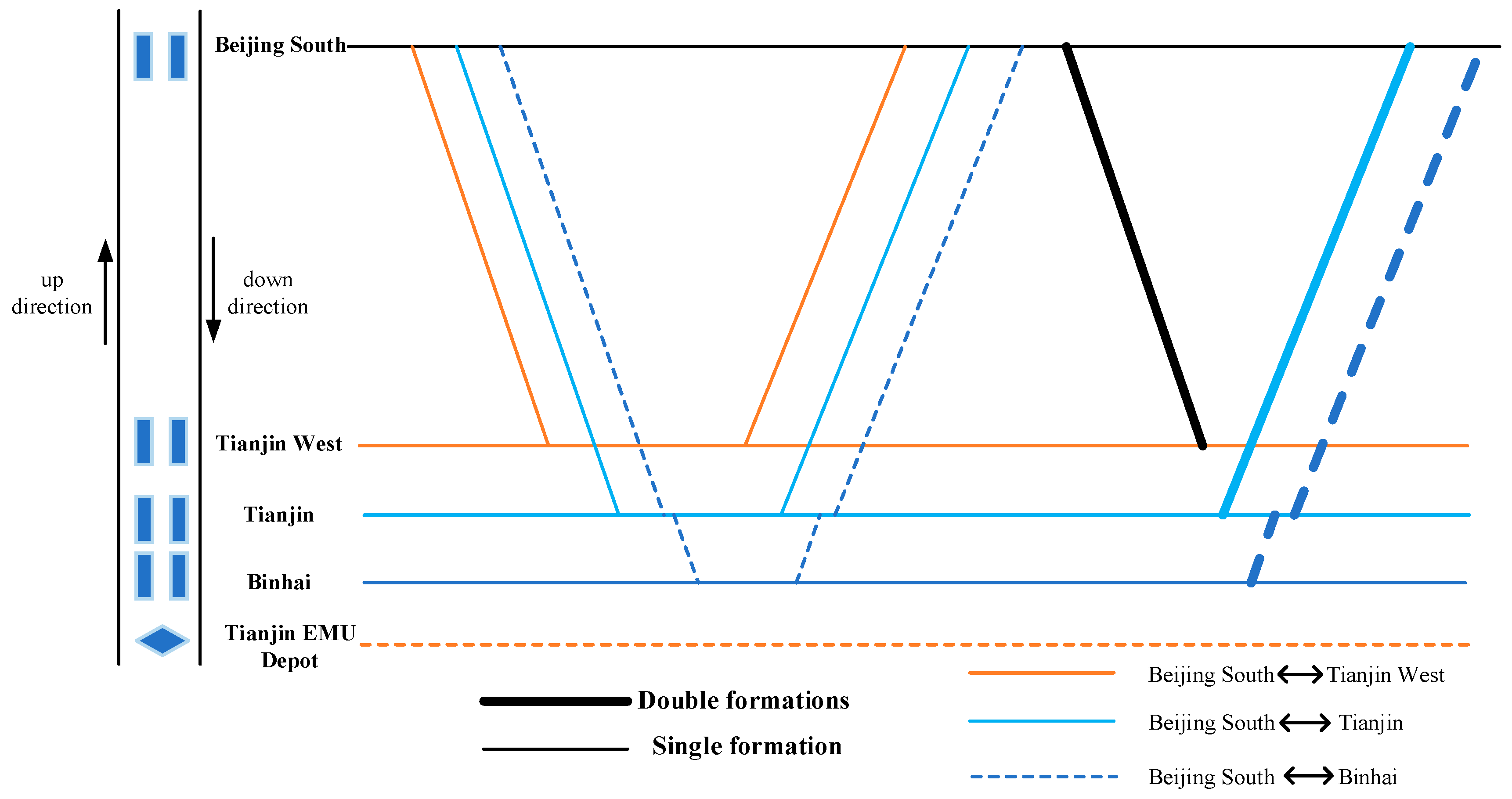
A real-world case study of the Beijing–Tianjin IHSR in China is introduced to verify the feasibility of the proposed model. Additionally, compared with the fixed formation mode, this shows that the flexible formation mode can effectively save cost and improve the utilization rate of the rolling stock.

3. Problem Description

3.1. Problem Description

IHSR trains mainly connect two neighboring cities, and a fixed-segment rolling stock scheduling mode is adapted. In contrast with long-distance HSR trains, IHSR trains operate with high frequency and can even reach the mode of bus operation, mainly serving passengers commuting between two neighboring cities. The passenger demand of IHSR also presents unique characteristics, with a certain regularity and volatility; a significant difference in passenger demand between weekdays and holidays; a higher passenger demand in peak hours on weekdays than in other periods; and an obvious difference in passenger demand between the up direction and down direction. At the same time, because IHSR trains have the characteristics of high frequency, short intervals, and short distances, passenger demand is not very precise regarding the choice of departure time, only the need to complete the journey within a certain period.

According to the characteristics of the passenger demand of IHSR trains, we put forward a flexible train formation mode based on passenger demand. That is, the total train formations in a certain time period can meet passenger demand, but the specific formation of each train is flexible and can be adjusted according to the rolling stock scheduling so as to better adapt to the passenger demand and improve the train occupancy rate. Therefore, the optimization of the rolling stock scheduling problem in this paper not only involves the determination of the best formation of each train but also considers how to allocate EMU rolling stock to each train based on passenger demand so as to reduce operating costs and improve the utilization efficiency of rolling stocks on the basis of completing transport tasks.

In order to better illustrate the problem studied in this paper, we take a fixed-segment rolling stock scheduling case as an example. Suppose that there is an IHSR line connecting two cities, which has four main stations and two EMU depots, as shown in Figure 1. There are two main types of train formations—namely, single formation with eight cars and double formations with 16 cars. Trains can directly handle turnaround operations at these four stations. Additionally, for trains with different numbers of formations, they need to enter the EMU depot for coupling/decoupling operations before turnaround. All trains must return to the EMU depot at night for maintenance after completing their transportation tasks during the day.

As shown in Figure 1, the train formations are variable; therefore, there are four types of turnaround operations: (a) single formation connecting to single formation, (b) double formations connecting to double formations, (c) single formation connecting to double formations, and (d) double formations connecting to single formation. Types (a) and (b) can be carried out directly at the station, while for (c) and (d) coupling/decoupling operations in the EMU depot need to be executed. At the same time, trains can run between each station in the up and down directions, so there are various train routes—namely, Station 1↔Station A, Station 1↔Station B, Station 2↔Station a, Station 2↔Station B. Therefore, the variable train formations and the multiple routes lead to a wide array of rolling stock scheduling schemes. The question of how to choose the most reasonable scheme out of many possible schemes is the key problem for dispatchers and is of great significance for helping railway departments to save cost.

Based on the above analysis, combined with the relationship between passenger demand and train formations, we put forward the concept of flexible train formation by time period and establish an integrated optimization model of EMU rolling stock scheduling and flexible train formation based on passenger demand.

The flexible train formation by time period is defined as follows. According to the time specified in the timetable, the trains travelling within a certain time period are aggregated and classified. In each time period, the total formations of the trains are fixed, but the formations of the individual trains are variable. A flexible train formation does not change the existing timetable, meaning that passenger demand with a high accuracy of travel time can be met. At the same time, the total train formations within the time period are fixed, and the other passenger demand with a relatively low accuracy of travel time can also be met.

3.2. Assumptions

To facilitate the establishment of a mathematical model to solve the research problem, the following assumptions are proposed:

Assumption 1.

There is only one type of train running in the interval—that is, the turnaround and coupling/decoupling operations between trains are not affected by the types of train involved.

Assumption 2.

Multiple route sections are involved in the interval, the passenger demands between different route sections do not affect each other, and the passenger demands between different route sections are independent of each other, meaning that the aggregation of passenger demand in different time periods is carried out according to each route section.

Assumption 3.

The passenger demand of each time period is known—that is, it is assumed that the rolling stock scheduling is based on an accurate passenger demand forecast for each time period.

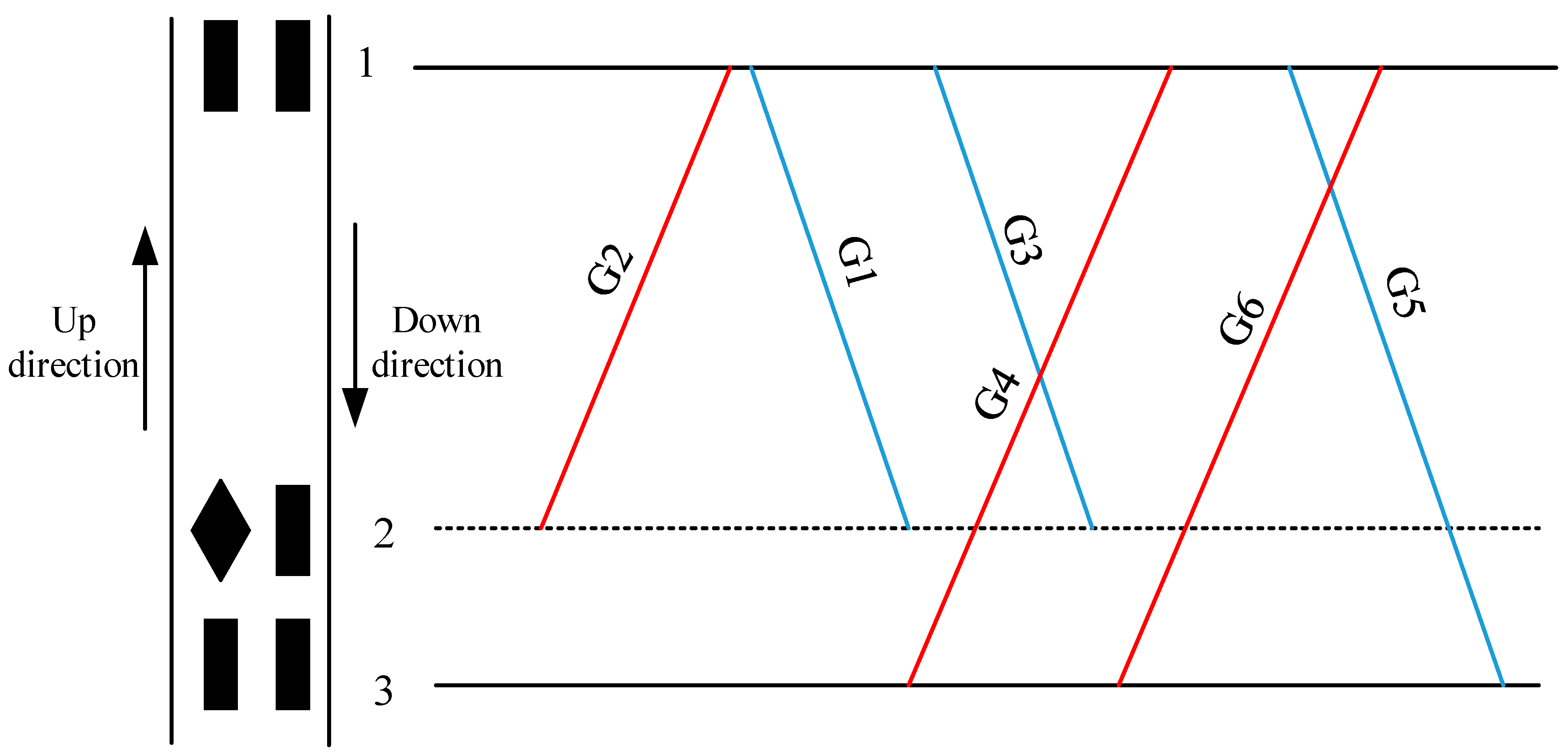
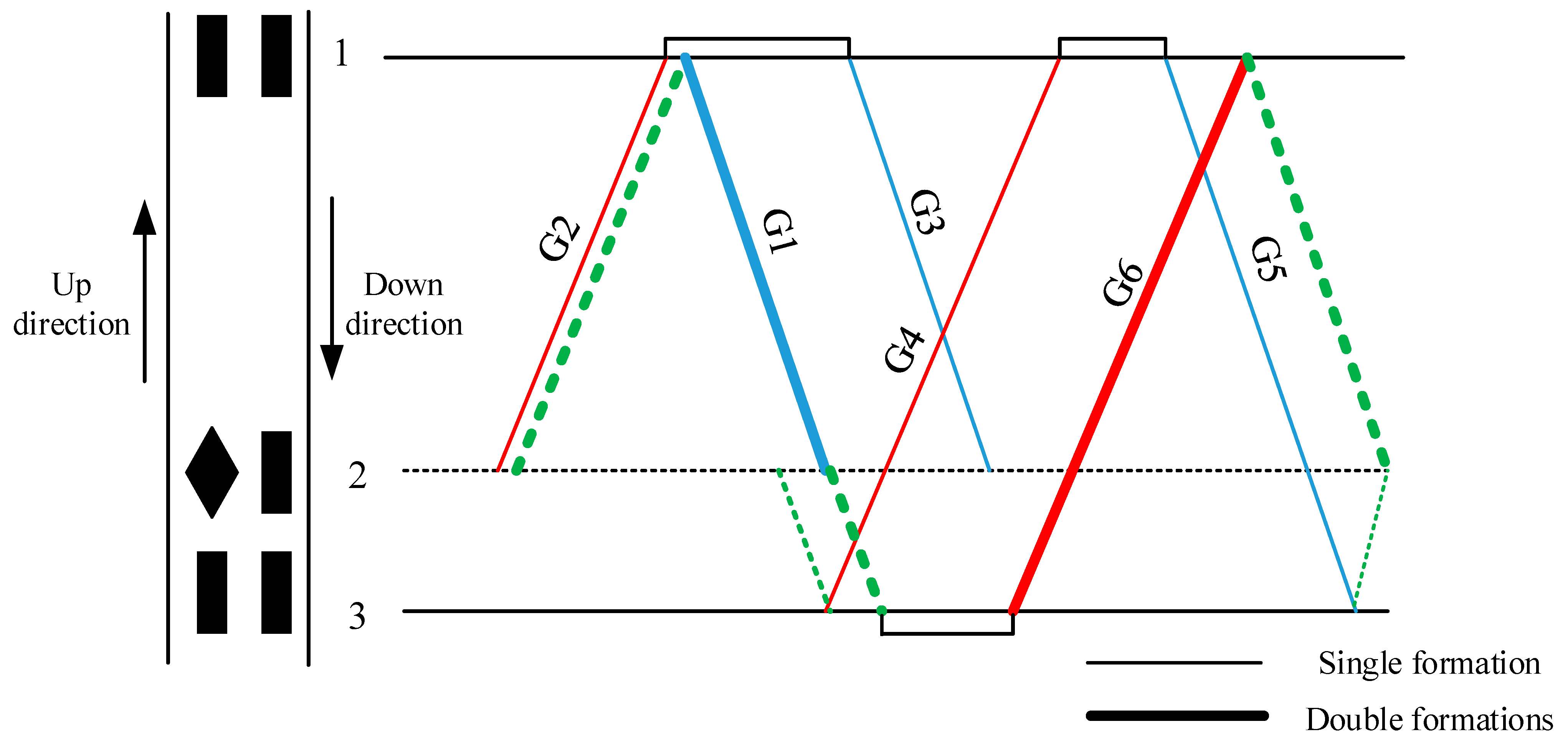
3.3. Illustration Example

We give an example to better illustrate the integrated optimization problem of rolling stock scheduling and flexible train formation. As shown in Figure 2, an IHSR line covers three stations, of which Station 2 is directly connected to the EMU depot. Six trains are running on the segment, with three going in each direction. The arrival and departure stations of each train are shown in Figure 2. The timetable and flexible train formation relationships based on passenger demand are shown in

Table 2. Basic information about the trains in the small IHSR case.

Trains	Departure Time	Departure Station	Arrival Time	Arrival Station	Train Formation
G1	9:10	1	9:40	2	3
G3	10:00	1	10:30	2
G5	11:20	1	12:20	3	1
G2	9:00	2	9:30	1	1
G4	9:50	3	10:50	1	3
G6	10:40	3	11:40	1

.

As shown in Table 2, the timetable is known, and the train formations are flexible according to passenger demand. For example, the total formations of the G1 and G3 trains are greater than or equal to 3, meaning that there are three possible formation schemes for these two trains as follows: ➀ G1 = 1, G3 = 2; ➁ G1 = 2, G3 = 1; ➂ G1 = 2, G3 = 2. Similarly, G4 and G6 also have three feasible formation schemes for meeting passenger demand. According to the above train and route information, by setting a certain connection time requirement, the train formation and rolling stock scheduling scheme can be obtained, as shown in Figure 3. The thin lines in the figure represent single formation, the thick lines represent double formations, and the green dotted lines represent deadhead trains.

It can be seen from the results in Figure 3 that the purpose of the integrated optimization of rolling stock scheduling and flexible train formation in this paper is to determine a reasonable train formation and rolling stock connection scheme.

Therefore, the optimization problem of the rolling stock scheduling plan in fixed-segment mode can be described as follows. On the premise of the established timetable and passenger demand; considering constraints such as different connection methods, train formations, and sources of rolling stocks; and aiming at achieving the minimum operation cost of rolling stocks, an integrated optimization model of rolling stock scheduling and flexible train formation based on passenger demand is constructed so as to obtain the best rolling stock scheduling plan.

4. Mathematical Model

4.1. Notations

The sets, parameters, and variables used in the model are shown in

Table 3. Sets, parameters, and variables of the model.

Sets	Description
$I$	Set of all trains.
$S$	Set of all stations.
$R$	Set of all route sections.
$T$	Set of all time periods.
$K$	Set of directions. When $k=0$, it represents the up direction. When $k=1$, it represents the down direction.
$I_t^k$	Set of trains in the $t$th time period in $k$ direction.
Parameters	Description
$t^{\min }$	The minimum time for the train to turn around directly at the station.
${\gamma }^{\min }$	The minimum time for the train to turn around after coupling/decoupling in the EMU depot.
$d_i$	The departure time of train i.
$a_i$	The arrival time of train i.
$t^{ia\to jd}$	The travel time from the arrival station of train i to the departure station of train j.
$t^{ia\to D}$	The travel time from the arrival station of train i to the EMU depot.
$t^{D\to jd}$	The travel time from the EMU depot to the departure station of train j.
${\phi }_1$	The weight of rolling stock cost.
${\phi }_2$	The weight of rolling stock coupling/decoupling cost.
${\phi }_3$	The weight of rolling stock deadhead cost.
$p_{t,r}^k$	The total passenger demand of $t$th time period in the $r$ route section of $k$ direction.
${\delta }_{i,r}^k$	The occupancy rate of train $i$ in $r$ route section of $k$ direction.
$c$	The number of passengers that can be carried by a single formation.
Variables	Description
$Z$	Objective function value.
$NR$	The number of rolling stocks.
$NC$	The number of coupling/decoupling times.
$ND$	Total deadhead time.
$x_i$	The formation of train $i$, 1 indicates single formation, and 2 indicates double formations.
$x_{i,r}^k$	The formation of train $i$ in $r$ route of $k$ direction, 1 indicates single formation, and 2 indicates double formations.
$y_{D,i}$	The number of rolling stocks of train $i$ directly provided by the EMU depot.
$y_{i,D}$	The number of rolling stocks that train $i$ directly returns to the EMU depot for repair and maintenance.
${\alpha }_{i,j}$	Binary variable, if train $j$ connect with train $i$ in the station directly, ${\alpha }_{i,j}=\hspace{0.17em}1$, otherwise, ${\alpha }_{i,j}=\hspace{0.17em}0$.
${\beta }_{i,j}$	Binary variable, if train $j$ connect with train $i$ after coupling/decoupling operations in the EMU depot, ${\beta }_{i,j}=\hspace{0.17em}1$, otherwise, ${\beta }_{i,j}=\hspace{0.17em}0$.

.

4.2. Optimization Objectives

The purpose of the optimization in this paper is to reduce the operation cost of rolling stocks. Among the operation costs of rolling stocks, the largest cost is the cost of purchasing rolling stocks—that is, the number of rolling stocks. At the same time, every coupling and decoupling operation will consume a certain amount of time and money. In addition, there will be additional costs to consider in the case of deadhead running between stations or between EMU depots and stations. Based on this, the optimization objectives of the model include three aspects:

➀ The number of rolling stocks, as shown in Equation (1). ➁ The number of coupling/decoupling operations needed, as shown in Equation (2). ➂ The deadhead time, as shown in Equation (3). To facilitate solving the multi-objective optimization model, the multiple objectives are transformed into a single objective using linear weighting, as shown in Equation (4). Since the weight coefficient of the objective function has a certain influence on the objective result, the value of the weight is considered comprehensively in combination with the actual application situation and relevant literature research.

$$NR={\displaystyle \sum _{i=1}^I{x}_{D,i}}$$

(1)

$$NC={\displaystyle \sum _{i=1}^I{\displaystyle \sum _{j=1}^I{\beta }_{i,j}}}$$

(2)

$$ND={\displaystyle \sum _{i=1}^I{\displaystyle \sum _{j=1}^I\left({\alpha }_{i,j}\ast t^{ia\to jd}\right)}}+{\displaystyle \sum _{i=1}^I{\displaystyle \sum _{j=1}^I\left[{\beta }_{i,j}\ast \left(t^{ia\to D}+t^{D\to jd}\right)\right]}}$$

(3)

$$\begin{array}{cc}\min & Z={\phi }_1\ast NR+{\phi }_2\ast NC+\end{array}{\phi }_3\ast ND$$

(4)

4.3. Constraints

This model mainly includes four constraints: constraints of different turnaround and connection types, constraints of the origin and destination of rolling stocks, constraints of the balance of rolling stocks, and constraints of flexible train formations by time period. The following is a detailed introduction to each type of constraint.

(1)

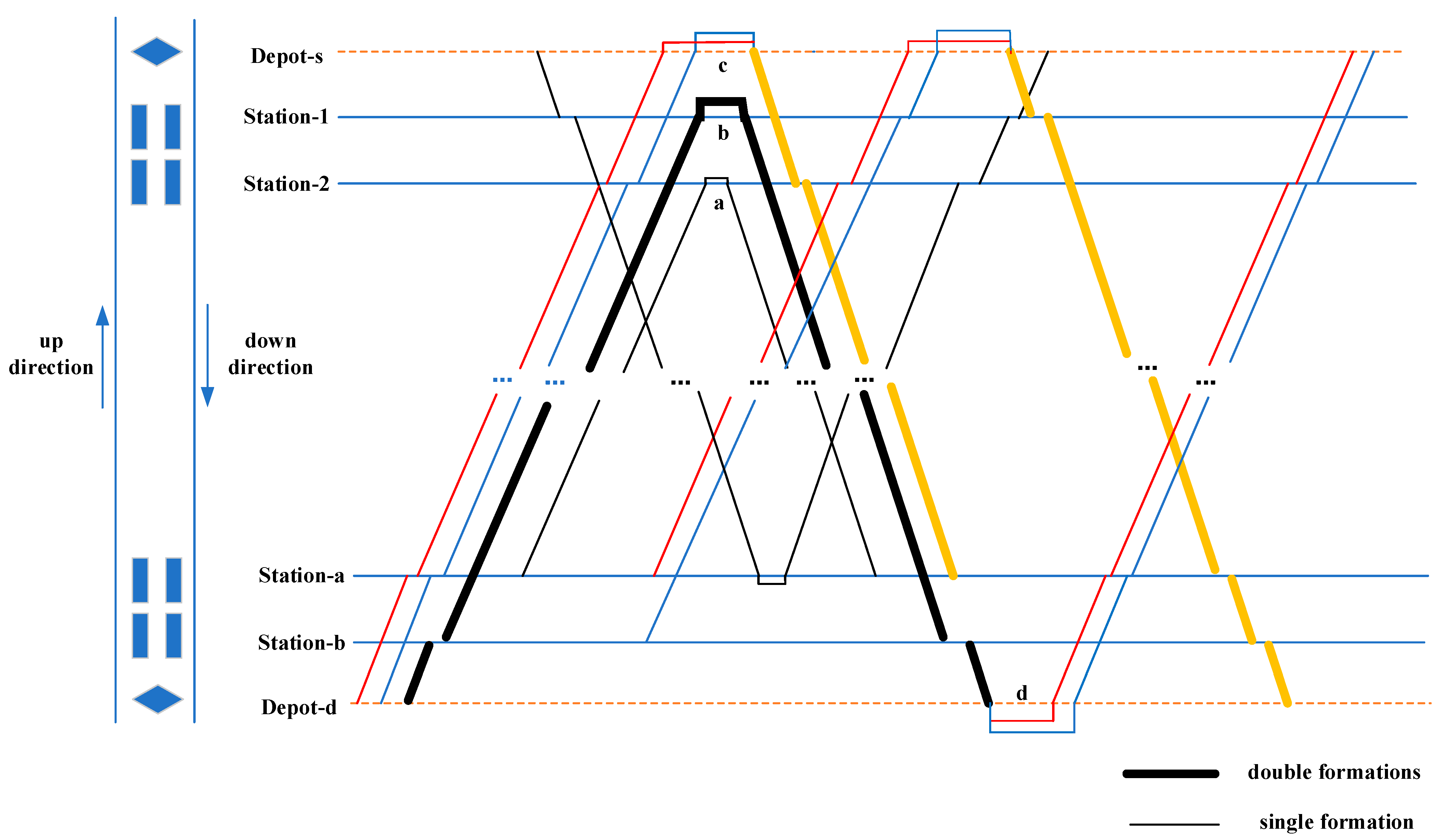
Constraints on different train connection types.

There are two turnaround and connection types between trains: One is that the same formation trains directly turn around and connect at the station, the other is that different formation trains turn around and connect after coupling/decoupling at the EMU depot. Different turnaround and connection types have different constraints.

➀

Direct turnaround and connection at the station.

Two trains with the same formation can turn around and connect directly at the station as long as the interval time meets the connection time requirement of the station, as shown in Formulas (5) and (6).

$${\alpha }_{i,j}\le 1-\left|x_i-x_j\right|\hspace{1em}\forall i\in I,j\in I$$

(5)

$$d_j-a_i\ge t_{\min }+t^{ia\to jd}-M\ast \left(1-{\alpha }_{i,j}\right)\hspace{1em}\forall i\in I,j\in I$$

(6)

Formula (5) indicates that two trains must have the same train formation for turning around and connecting at the station. Formula (6) indicates that the interval time of the two trains is not less than the sum of the minimum time for trains to turn around directly at the station and the deadhead running time.

➁

Turnaround and connection after entering the EMU depot with coupling/decoupling operations.

As the station cannot handle coupling/decoupling operations, trains with different formations cannot directly turn around and connect at the station and need to enter the EMU depot for coupling/decoupling. Similarly, for trains that turn around and connect after entering the EMU depot with coupling/decoupling operations, Formulas (7) and (8) should be satisfied.

$${\beta }_{i,j}\le \left|x_i-x_j\right|.\forall i\in I,j\in I$$

(7)

$$d_j-a_i\ge {\gamma }_{\min }+t^{ia\to D}+t^{D\to jd}-M\ast \left(1-{\beta }_{i,j}\right)\hspace{1em}\forall i\in I,j\in I$$

(8)

Formula (7) indicates that the trains that turn around and connect after entering the EMU depot for coupling/decoupling must have different formations. Formula (8) indicates that the interval time between the two trains is not less than the sum of the time of the coupling/decoupling operations and the time of the two trains entering and exiting the EMU depot.

(2)

Constraints on the origin and destination of rolling stocks.

For all EMU trains in the model, the rolling stocks come from the EMU depot, and after completing all train tasks the rolling stocks will also return to the EMU depot for repair and maintenance. However, for an individual EMU train, there are many situations that can arise regarding the origin and destination of rolling stocks. Formulas (9) and (10) represent the origin and destination of rolling stocks for an individual train.

$$x_i={\displaystyle \sum _{j=1}^I\left({\alpha }_{j,i}\ast x_j\right)}+{\displaystyle \sum _{j=1}^I{\beta }_{j,i}}+y_{D,i}\hspace{1em}\forall i\in I$$

(9)

$$x_i={\displaystyle \sum _{j=1}^I\left({\alpha }_{i,j}\ast x_j\right)}+{\displaystyle \sum _{j=1}^I{\beta }_{i,j}}+y_{i,D}\hspace{1em}\forall i\in I$$

(10)

Formula (9) indicates that the rolling stocks mainly come from three aspects:

a.

The train turning around directly at the station.

b.

The train turning around after entering the EMU depot with coupling/decoupling operations.

c.

The EMU depot.

Formula (10) indicates that the rolling stocks are mainly bound for three aspects:

a.

Turning around directly with other EMU trains at the station.

b.

Turning around with other EMU trains after entering the EMU depot with coupling/decoupling operations.

c.

Going to the EMU depot for repair and maintenance.

(3)

Constraints on the balance of rolling stocks.

In addition to IHSR trains, each station also handles the stopping operations of other types of trains, meaning that all trains have to return to the EMU depot for repair and maintenance after completing their transportation tasks at night. The number of rolling stocks going into and out of the EMU depot has to be kept in check, as shown in Formula (11).

$${\displaystyle \sum _{i=1}^I{y}_{i,D}}={\displaystyle \sum _{i=1}^I{y}_{D,i}}$$

(11)

(4)

Constraints on flexible train formation by time period based on passenger demand.

The flexible train formation by time period combines the passenger demand and train formation. The premise is that the train formations should meet the total passenger demand in each time period, as shown in Formula (12).

$$p_{t,r}^k\le {\displaystyle \sum _{i=1}^{I_t^k}{x}_{i,r}^k}\ast c\ast {\delta }_{i,r}^k\hspace{1em}\forall t\in T,r\in R,k\in K$$

(12)

Formula (12) indicates that the total number of train formations in each time period in the same direction and same route must meet the total passenger demand in that time period.

4.4. Linearization Process

The constructed model is a mixed-integer nonlinear programming model, and the objective function involves three aspects, making it a multi-objective optimization problem where the importance of different objectives is determined by the weight coefficients. At the same time, the model involves multiple constraints, among which some constraints are nonlinear and cannot be solved directly by a linearization solver. In order to solve the model directly using the linearization solver, the nonlinear constraints are linearized as follows.

➀

Formula (5).

In Formula (5), both $x_i$ and $x_j$ are binary decision variables, and the $\left|x_i-x_j\right|$ results in the nonlinear constraint condition. Formula (5) can be transformed into Formulas (13) and (14) for linearization.

$${\alpha }_{i,j}\le 1+\frac{x_i-x_j}{2}\hspace{1em}\forall i\in I,j\in I$$

(13)

$${\alpha }_{i,j}\le 1+\frac{x_j-x_i}{2}\hspace{1em}\forall i\in I,j\in I$$

(14)

➁

Formula (7).

For Formula (7), the same method as Formula (5) can be used to transform Formula (7) into Formulas (15) and (16) for linearization.

$${\beta }_{i,j}\le 4-x_i-x_j\hspace{1em}\forall i\in I,j\in I$$

(15)

$${\beta }_{i,j}\le x_i+x_j-2\hspace{1em}\forall i\in I,j\in I$$

(16)

After the above linearization process, the problems studied can be solved by the linearization solver. The Gurobi solver can solve large-scale linear problems, quadratic problems, mixed-integer linear problems, and other mathematical optimization problems well. At the same time, The Gurobi solver has a rich interface and a faster optimization speed and accuracy. Therefore, this paper selects the Gurobi solver to solve the model.

5. A Real-World Instance: Beijing-Tianjin IHSR

In this part, the Beijing–Tianjin IHSR in China is selected for an example study. In order to verify the feasibility and validity of the proposed model, we consider two train formation modes. Additionally, a comparative analysis is also carried out based on the number of rolling stocks, the number of coupling/decoupling operations, the utilization rate of rolling stock, etc.

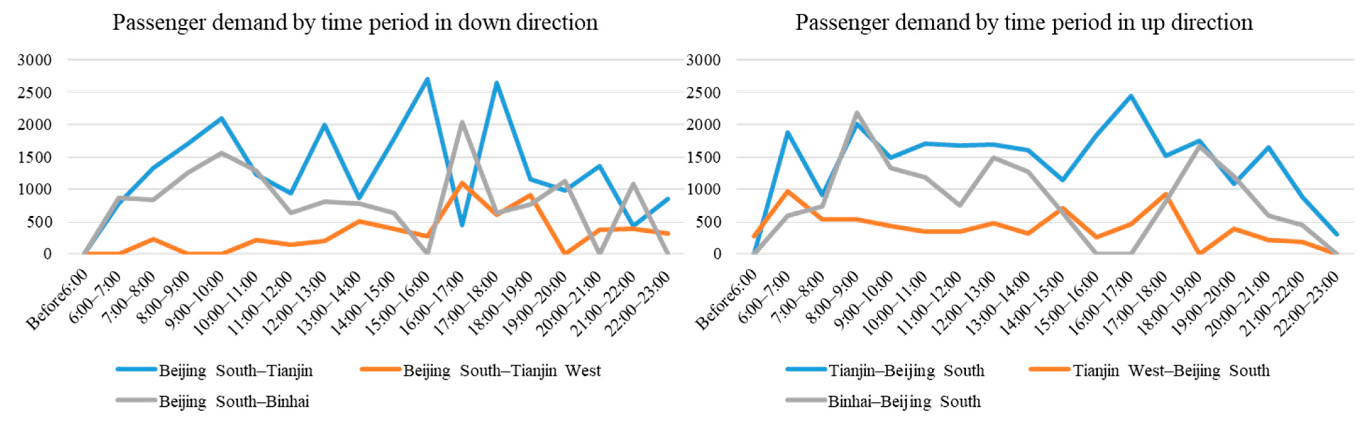
5.1. Instance Description

The Beijing–Tianjin IHSR line is 166 km long, with seven stations along the way, of which Beijing South, Tianjin, Tianjin West, and Binhai handle the origin and destination operations, as shown in Figure 4. The rolling stocks in this segment adopt a fixed-segment rolling stock scheduling mode, and all the rolling stocks are provided by the Tianjin EMU depot. Since August 2018, all Beijing–Tianjin IHSR trains have used “Fuxing” EMU trains, and there are two types of train formations, which are double formations with 16 cars and single formation with eight cars.

The daily timetable is known before the rolling stock scheduling is determined. According to the fluctuation of passenger demand, Beijing–Tianjin IHSR trains currently use a total of six different types of timetables. Except for Tuesday, Wednesday, and Thursday, when a unified weekday timetable is used, the timetables of the other days are all different. The passenger demand data for a weekday are used in this study, and the passenger demand date of each route during each time period are shown in Figure 5.

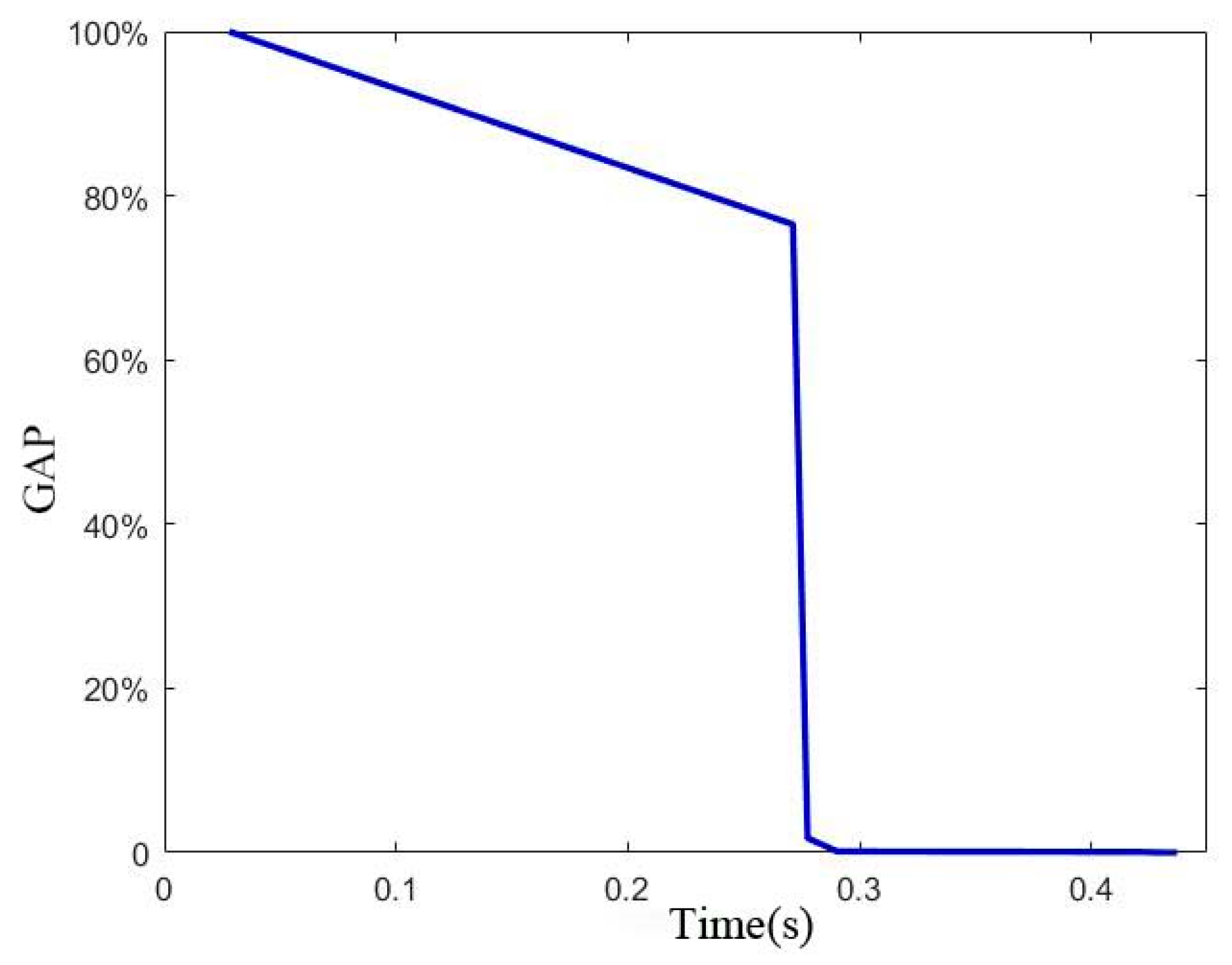
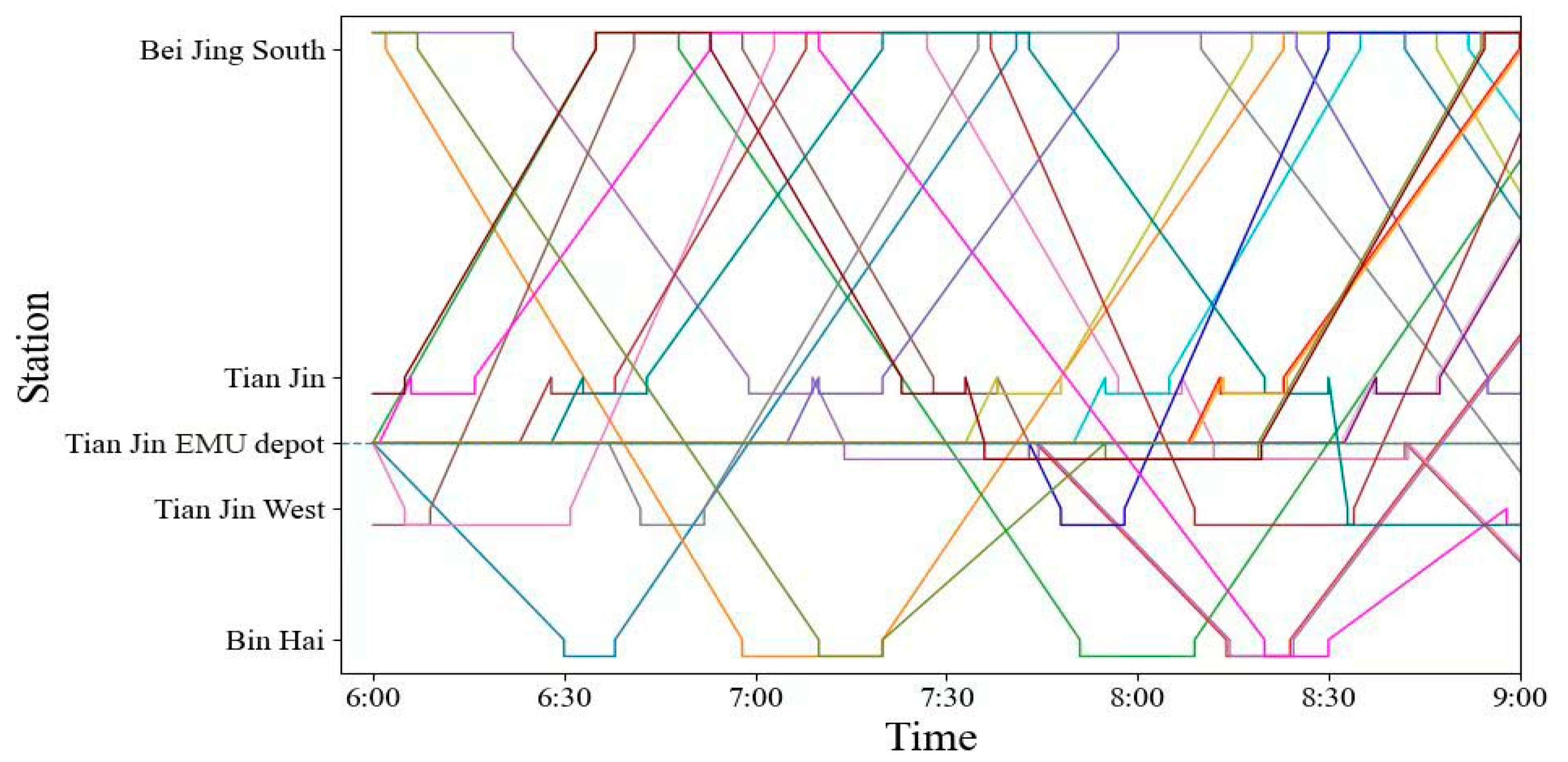
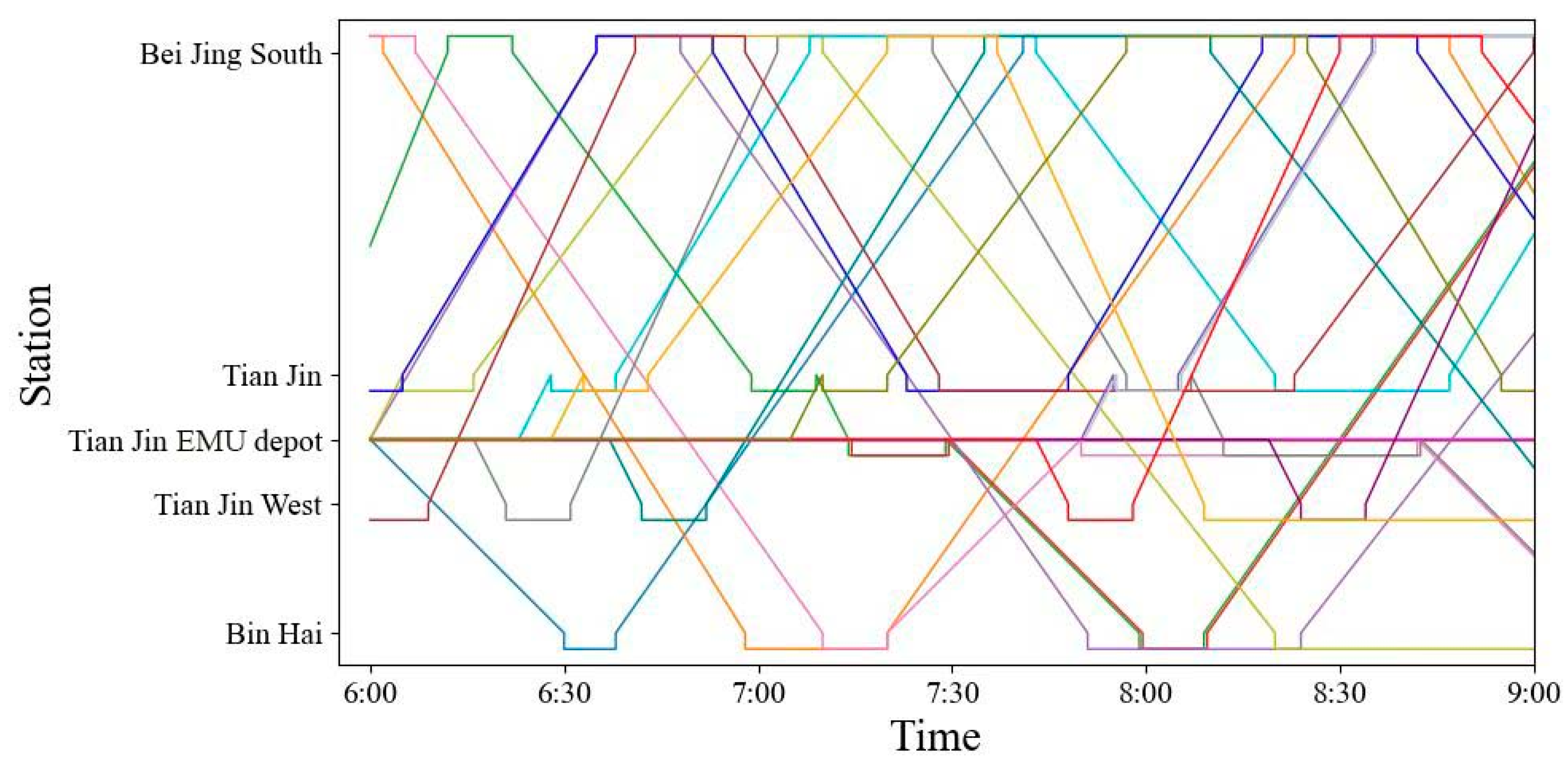
5.2. Results and Analysis

The above-mentioned passenger demand for the Beijing–Tianjin IHSR was used in the constructed model for calculation. In the objective function, the cost of the deadhead time was taken as the benchmark and set to 1; since the coupling/decoupling takes 30 min, the coupling/decoupling cost weight was set to 30 according to its time consumption. The model focuses on the rolling stock cost, which is also the most important part of the objective function, and through sensitivity analysis it was found that when the rolling stock cost weight is above 100, the number of rolling stocks is always maintained at a minimum level. Combined with the actual cost consumption of the EMU depot, the weight of the rolling stock cost was set to 200. In addition, the weight value of the objective function also depends on the actual transportation organization strategy used. By adjusting the weight value of the objective function, the efficiency of rolling stock utilization under different transportation organization strategies can be analyzed. Other related parameters were used according to the actual situation of the Beijing–Tianjin IHSR, as shown in

Table 4. Parameter values for the case study.

Parameter	Value	Parameter	Value	Parameter	Value
$t^{\min }$	15 min	${\phi }_1$	200	${\delta }_{i,r}^k$	Actual value
${\gamma }^{\min }$	30 min	${\phi }_2$	30	$d_i$	Actual value by timetable
$c$	576	${\phi }_3$	1	$a_i$	Actual value by timetable

and

Table 5. Deadhead time parameters for case study.

O/D	Beijing South	Tianjin	Tianjin West	Binhai	EMU Depot
Beijing South	0	32 min	35 min	70 min	35 min
Tianjin	32 min	0	3 min	25 min	5 min
Tianjin West	35 min	3 min	0	28 min	5 min
Binhai	70 min	25 min	28 min	0	30 min
EMU depot	35 min	5 min	5 min	30 min	0min

.

The Gurobi solver was used to solve this instance. The computer environment was [email protected] GHz and the RAM was 16 GB. The calculation of the fixed train formation mode and the flexible train formation mode of the rolling stock scheduling plan was performed separately. In the fixed formation mode, only the optimal connection scheme between trains needs to be solved, the calculation scale was relatively small, and the optimal solution could be obtained in a very short time. While in the flexible formation mode, the optimal train formation scheme and the optimal connection scheme between trains need to be solved, and the two also affect each other, the calculation process was more time-consuming, the optimal solution could be obtained within 3 min. The calculated “GAP-time” relationships are shown in Figure 6 and Figure 7.

As can be seen in Figure 6 and Figure 7, in the fixed formation mode, the GAP value reaches 0% after 0.4 s. In the flexible formation mode, the GAP value reaches within 1% after 106 s and reaches 0% after 121 s. The “GAP-time relationships” results in both modes show that the results obtained with the Gurobi solver are optimal. After optimization, the rolling stock scheduling schemes are shown in Figure A1 and Figure A2, and the details of the turnaround and connection relationships are shown in the

Table A1. Turnaround and connection relationships of EMU trains.

Rolling Stock	Fixed Train Formation Mode	Flexible Train Formation Mode
1	C2552, C2561, C2562, C2029, C2036, C2579, C2058, C2061, C2226, C2591, C2596, C2669	C2552, C2563, C2564, C2031, C2038, C2579, C2582, C2649, C2674, C2089
2	C2551, C2554, C2019, C2024, C2617, C2638, C2039, C2042, C2049, C2050, C2059, C2224, C2071, C2076, C2671	C2551, C2554, C2015, C2020, C2569, C2576, C2631, C2652, C2643, C2666, C2651
3	C2555, C2556, C2565, C2566, C2621, C2642, C2629, C2652, C2641, C2588, C2653	C2201, C2556, C2565, C2055, C2587
4	C2558, C2583	C2556, C2565, C2055, C2587
5	C2201, C2558, C2583	C2555, C2558, C2613, C2632, C2619, C2640, C2583, C2584
6	C2610, C2005, C2560, C2213, C2587	C2630, C2209, C2034, C2621, C2642, C2583, C2584
7	C2614, C2009, C2560, C2213, C2587	C2553, C2560, C2051, C2059, C2224
8	C2616, C2559, C2564, C2031, C2040, C2053, C2056, C2649, C2668, C2657	C2614, C2009, C2560, C2051, C2059, C2224
9	C2008, C2015, C2020, C2569, C2568, C2627, C2648, C2635, C2660, C2647, C2674, C2661	C2202, C2557, C2562, C2617, C2638, C2041, C2044, C2213, C2052, C2639, C2664, C2223, C2080, C2087, C2090
10	C2010, C2205, C2022, C2571, C2570, C2625, C2646, C2060, C2589, C2592, C2595	C2004, C2203, C2014, C2207, C2566, C2037, C2218, C2581, C2058, C2061, C2226, C2591, C2596, C2669
11	C2622, C2567, C2572, C2045, C2048, C2057, C2222	C2002, C2003, C2008, C2561, C2568, C2623, C2644, C2629, C2650, C2641, C2064, C2593, C2594, C2661
12	C2004, C2605, C2624, C2017, C2210, C2027, C2034, C2577, C2578, C2222	C2610, C2005, C2208, C2567, C2570, C2045, C2048, C2633, C2588, C2655
13	C2202, C2557, C2626, C2025, C2032, C2037, C2576, C2631, C2650, C2639, C2062, C2221, C2074, C2597	C2626, C2571, C2572, C2625, C2646, C2057, C2222, C2071, C2076, C2083, C2086
14	C2204, C2203, C2628, C2613, C2632, C2619, C2640, C2047, C2220, C2637, C2586, C2593, C2594, C2089	C2616, C2559, C2210, C2027, C2032, C2577, C2578, C2637, C2660, C2647, C2668, C2077, C2230, C2093
15	C2206, C2013, C2018, C2023, C2030, C2033, C2214, C2623, C2644, C2055, C2054, C2643, C2664, C2651, C2678, C2091	C2010, C2019, C2026, C2573, C2574, C2053, C2056, C2217, C2062, C2221, C2074, C2671
16	C2014, C2207, C2212, C2211, C2216, C2043, C2046, C2633, C2654, C2063, C2066, C2075, C2078, C2085, C2088	C2010, C2019, C2050, C2585, C2586, C2075, C2078, C2085, C2088
17	C2014, C2207, C2038, C2041, C2044, C2051, C2052, C2065, C2590, C2077, C2230, C2093	C2624, C2017, C2024, C2029, C2036, C2039, C2042, C2049, C2054, C2065, C2590, C2657
18	C2208, C2026, C2573, C2574, C2585, C2584	C2622, C2205, C2022, C2615, C2634, C2035, C2040, C2047, C2220, C2589, C2592, C2595
19	C2208, C2630, C2209, C2585, C2584	C2204, C2605, C2628, C2025, C2030, C2033, C2214, C2043, C2046, C2215, C2060, C2063, C2068, C2653, C2678, C2091
20	C2615, C2634, C2035, C2218, C2581, C2582, C2067, C2068, C2655	C2206, C2013, C2018, C2023, C2212, C2211, C2216, C2627, C2648, C2635, C2654, C2067, C2066, C2073, C2228, C2597
21	C2553, C2563, C2215, C2217, C2666, C2223, C2080, C2087, C2090
22	C2002, C2003, C2563, C2215, C2217, C2064, C2073, C2228, C2083, C2086

. The rolling stock scheduling schemes during the morning peak in both modes are shown in Figure 8 and Figure 9. The operation lines with the same color represent that they are served by the same rolling stocks in Figure A1, Figure A2, Figure 8 and Figure 9.

From the above results, it can be seen that the fixed train formation mode consumed 22 rolling stocks and the flexible train formation mode consumed 20 rolling stocks. In addition to the number of rolling stocks, there was also a major difference between the coupling/decoupling cost and deadhead cost in the two modes. In the next section, the costs and other indicators of the two modes are compared and analyzed.

5.3. Comparison and Analysis of Results

In order to further verify the effectiveness of the constructed model and the optimization effect of the proposed flexible train formation by time period on rolling stock scheduling, the results of the two modes were compared and analyzed from the two aspects of rolling stock operation cost and rolling stock operation efficiency.

(1)

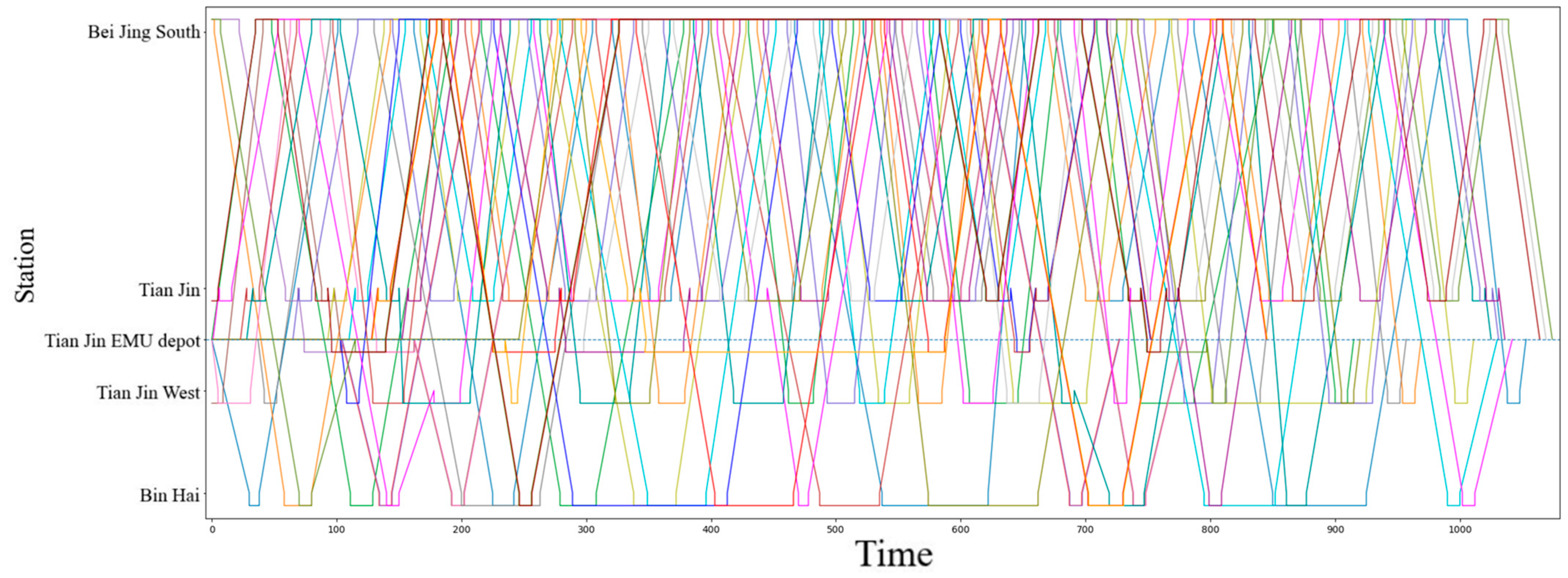
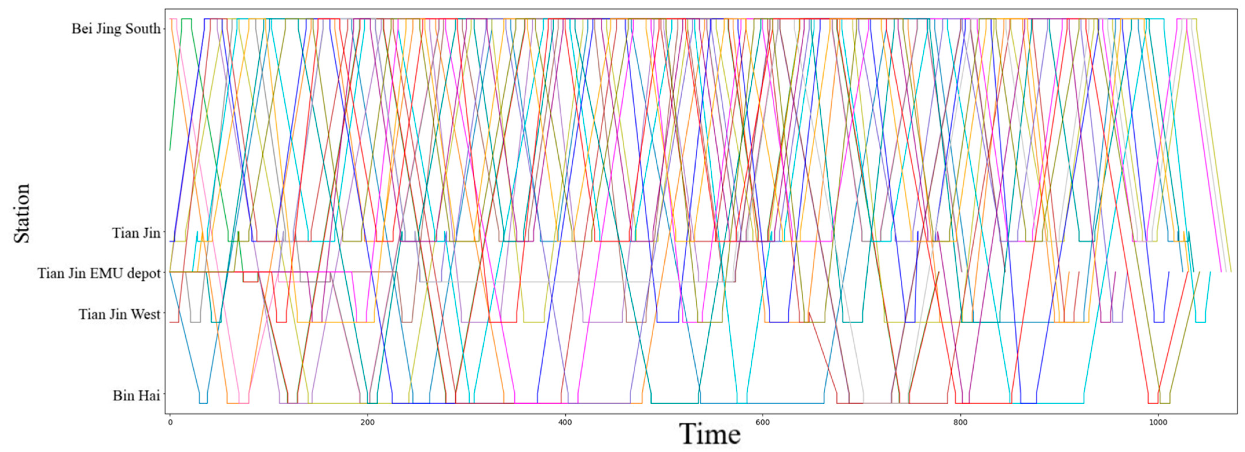
Comparison of rolling stock operation cost.

The objective values and costs for the two modes are shown in

Table 6. The objective values and costs in different modes.

Formation Mode	Direct Cost	Indirect Cost		Objective Value
	Number of Rolling Stocks	Number of Coupling/Decoupling	Deadhead Driving Time
Fixed formation	22	15	851 min	12,301
Flexible formation	20	7	550 min	10,760

.

As can be seen from the calculation results in Table 6, the objective function value decreased by 12.5% when the flexible formation mode was adopted. Both direct and indirect costs could be saved to a certain extent when the flexible formation mode was adopted.

In terms of direct cost, the flexible formation mode saved two rolling stocks. The purchase of rolling stock is expensive, and the rolling stock cost is the biggest cost expenditure in the rolling stock operation cost. The number of rolling stocks is a key factor to ensure the completion of transportation tasks, especially during holidays, when there may be a shortage of rolling stocks due to the surge in passenger transportation demand. In the case of this paper, the flexible train formation by time period essentially involved adjusting the train formations in each time period according to the passenger demand, then selecting the most cost-efficient train formation solution among many options. On this basis, the best rolling stock scheduling plan was developed.

In terms of indirect cost, both the number of coupling/decoupling and the deadhead time were significantly reduced in the flexible train formation mode compared with the fixed train formation mode, saving eight coupling/decoupling operations and 300 min of deadhead time, respectively. Beijing–Tianjin IHSR trains run in a high density, the connection between trains is very close, and there are few double formation trains, so most trains turn around and directly connect at the station and only a few trains enter the EMU depot to couple/decouple. Therefore, the number of coupling/decoupling operations was small in the two modes. Especially in the flexible formation mode, more trains with the same formation turned around and directly connected at the stations through optimization, which reduced the number of trains entering the EMU depot for coupling/decoupling.

There are two main types of deadhead trains. One is the deadhead running between two trains with different arrival and departure stations that turn around and directly connect at the station. The other is the deadhead running between the station and the EMU depot for trains that turn around and connect after entering the EMU depot for coupling/decoupling. In the flexible formation mode, a reduction in the number of coupling/decoupling leads to a reduction in the deadhead time, and more trains can turn around and directly connect at the station.

(2)

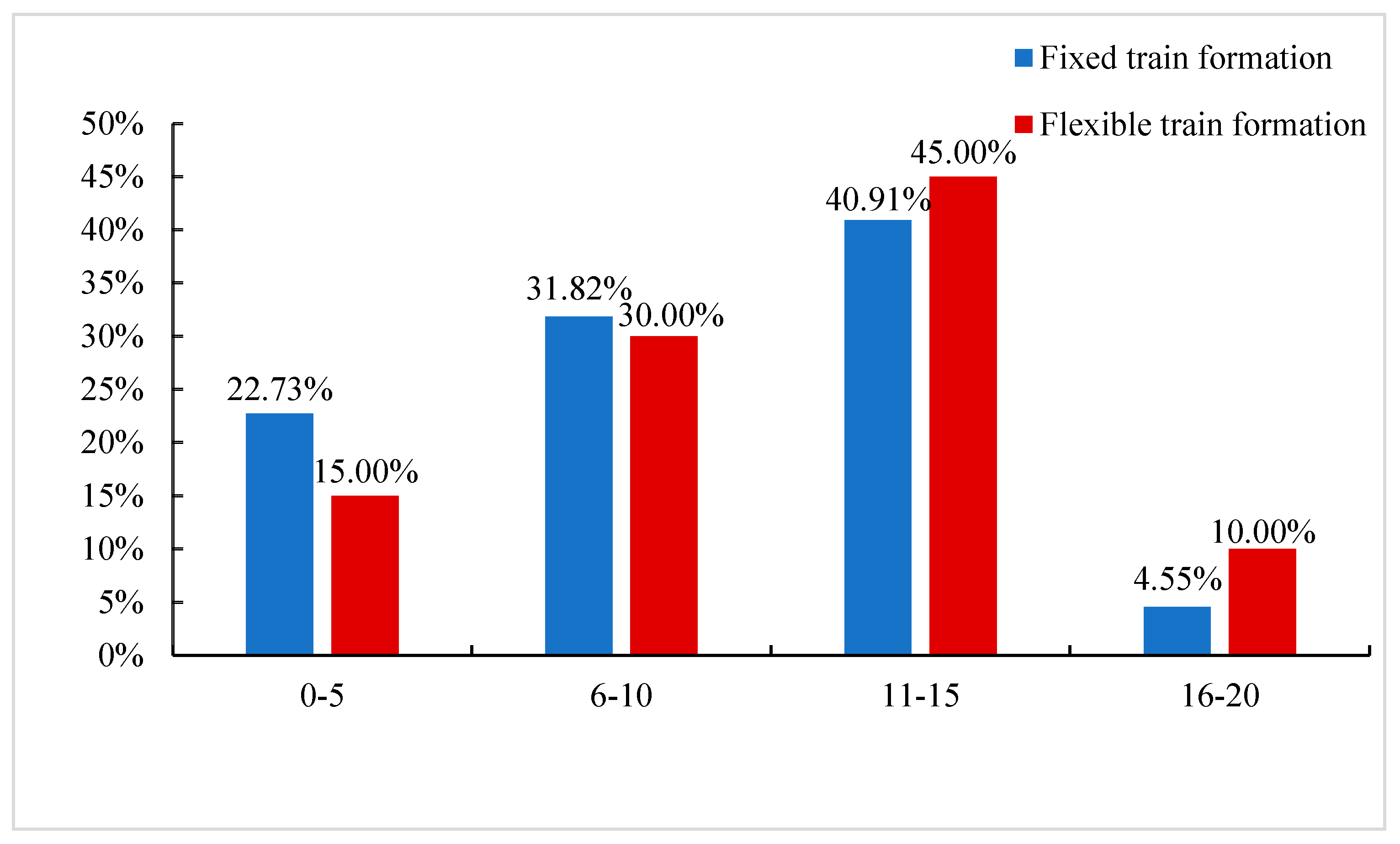
Comparison of rolling stock operation efficiency.

In order to further verify the optimization effect of flexible train formation on the rolling stock scheduling, other rolling stock operation efficiency indicators are calculated by combining the timetable and rolling stock scheduling scheme. These include the utilization rate of rolling stocks, the average number of tasks performed per rolling stock, and the balance of rolling stock utilization. The corresponding calculations are shown in Formulas (17)–(19); the meanings of the symbols used in the equation are shown in

Table 7. Meaning of calculation symbols.

Symbol	Meaning	Symbol	Meaning	Symbol	Meaning
$u^{\mathrm{total}}$	Total utilization of rolling stocks	$t_i^{\mathrm{in}}$	The time when the rolling stock $i$ returns to the depot	$e^{\mathrm{total}}$	Total number of rolling stocks
$u_i$	Operating time of rolling stock $i$	$o^{\mathrm{avg}}$	Average number of tasks performed per rolling stock	$\delta$	Balance degree of rolling stock scheduling
$t_i^{\mathrm{out}}$	The time when the rolling stock $i$ leaves the depot	$I^{\mathrm{total}}$	Total number of train tasks	$o_i$	Number of train tasks performed by rolling stock i

.

$$u^{\mathrm{total}}=\frac{{\displaystyle \sum u_i}}{{\displaystyle \sum \left(t_i^{\mathrm{out}}-t_i^{\mathrm{in}}\right)}}$$

(17)

$$o^{\mathrm{avg}}=\frac{I^{\mathrm{total}}}{e^{\mathrm{total}}}$$

(18)

$$\delta =\sqrt{\frac{{\displaystyle \sum {\left(o_i-o^{avg}\right)}^2}}{e^{\mathrm{total}}}}$$

(19)

Through calculation, the results of the three indicators in fixed formation mode and flexible formation mode are shown in

Table 8. Rolling stock operation efficiency values in different modes.

Formation Schemes	Rolling Stock Utilization	Average Number of Tasks Performed by Rolling Stocks	Balance Degree of Rolling Stock Scheduling
Fixed formation	65.30%	9.05	4.14
Flexible formation	68.12%	9.95	3.72

, and the corresponding distribution of the number of tasks performed by the rolling stock is shown in Figure 10.

As can be seen from the results in Table 8, there is little difference in the utilization rate between the two modes, with both reaching over 65%. This is due to the high density of the Beijing–Tianjin IHSR trains and the very short intervals between trains. In the peak hours, the interval between some trains can even reach less than 5 min. The high density leads to a high frequency of the turnaround of rolling stocks, and the rolling stocks are in a busy state most of the time, which leads to them having a high utilization rate. Compared with the fixed train formation mode, the trains in the flexible train formation mode are more closely connected and have less deadhead time, and their rolling stock utilization rate is 3% higher than that of the fixed train formation mode.

In terms of the average number of tasks performed by rolling stocks and the balance of rolling stock utilization, the flexible train formation is higher than the fixed train formation. Each rolling stock completes nearly one more train transport task on average, and the balance of rolling stock utilization is also significantly improved. For a single rolling stock, a minimum of four transport tasks are performed by a single rolling stock in flexible train formation mode, and a minimum of two transport tasks are performed by a single rolling stock in fixed train formation mode. As shown in Figure 7, the percentage of train tasks performed by a single rolling stock in the “0–5” and “6–10” ranges is greater for the fixed train formation mode, while the percentage of train tasks performed by a single rolling stock in the “11–15” and “16–20” ranges is greater for the flexible train formation mode. Therefore, in the flexible train formation mode, the difference in the number of tasks performed by each rolling stock is reduced and the balance of rolling stock utilization is increased, which not only helps to improve the utilization rate of the rolling stock but also facilitates the optimization of the maintenance plan of the rolling stock at night.

6. Conclusions and Further Research

In this paper, we propose the concept of flexible train formation by time period for the problem of rolling stock scheduling in fixed-segment mode. Based on this, an integrated optimization model of rolling stock scheduling and flexible train formation based on passenger demand is constructed and the model is solved using the Gurobi solver through linearization. Finally, the model is validated by a case of CHSR, and the following conclusions are drawn.

The proposed model is effective for the optimization of the rolling stock scheduling plan with a fixed-segment rolling stock scheduling mode, which aims at reducing the rolling stock operation cost and integrating the factors of passenger demand, rolling stock scheduling plan, and train formation plan.

The optimal results obtained for the flexible train formation and fixed train formation modes are compared, taking Beijing–Tianjin IHSR in China as a real-world instance. The results show that the flexible train formation mode can obtain certain savings over the fixed train formation mode in terms of both direct and indirect costs. In the Beijing–Tianjin IHSR case described in this paper, the flexible formation mode saves two rolling stocks and optimizes the objective value by 12.5% compared with the fixed formation mode. Additionally, by further comparing the efficiency indexes of rolling stock scheduling under the two modes, it is shown that the mode of flexible train formation by time period can improve the efficiency of rolling stock scheduling and optimize the balance of rolling stock utilization.

The optimization results show that the proposed integrated optimization model has improved the degree of matching between the train formation, rolling stock scheduling scheme, and passenger demand. It effectively alleviates the problem of there being insufficient capacity during the peak period and surplus capacity during the off-peak period, and improves resilience under external influences, which is important in order for the railway to achieve a cost reduction and efficiency increase.

In this paper, only the optimization of the rolling stock scheduling plan with fixed-segment mode was selected for research, which is applicable to IHSR lines. However, more regional areas of CHSR have adopted unfixed-segment rolling stock scheduling modes. The passenger demand fluctuates greatly throughout time and space in the unfixed-segment mode of rolling stock scheduling, leading to there being a more complicated relationship between passenger demand and rolling stock scheduling.

Our further research will focus on the following aspects. First, we will study the integrated optimization of passenger demand, train formation, and rolling stock scheduling plan further under the unfixed-segment rolling stock scheduling mode. Second, the train timetable is not immutable, and we can make the timetable flexible and integrate and optimize the timetable, rolling stock scheduling, and train formation with passenger demand. Extending our study with this integrated optimization will help to improve the applicability of the model. Finally, we will further explore how to adopt exact algorithms such as column generation and branch-price to solve the proposed model for larger-scale HSR network instances.

References

1. Zhao, P.; Hu, A. Research on the Circulating Optimization in the Condition of Using High·Speed Passenger Trains in Uncertain Railroad Region. J. Beijing Jiaotong Univ. 1997, 21, 621–624. [Google Scholar]
2. Nie, L.; Zhao, P.; Yang, H.; Hu, A.Z. Study on motor trainset operation in high-speed railway. J. China Railw. Soc. 2001, 23, 1–7. [Google Scholar]
3. Zhao, P.; Tomii, N. Train set scheduling and an algorithm. J. China Railw. Soc. 2003, 25, 1–7. [Google Scholar]
4. Zhao, P.; Tomii, N. An Algorithm for Train-set Scheduling on Weekday Based on Probabilistic Local Search. Syst. Eng.-Theory Pract. 2004, 2, 123–129. [Google Scholar]
5. Zhao, P.; Tomii, N. An Algorithm for Multiple-Bases Train-set Scheduling Based on Path-exchange. J. China Railw. Soc. 2004, 1, 7–11. [Google Scholar]
6. Zhang, C.C.; Chen, J.; Hua, W. Research on the EMU Operation Plan Based on Different Maintenance Capacity. China Railw. Sci. 2010, 31, 130–133. [Google Scholar]
7. Tong, L.; Nie, L.; Zhao, P. Application of Ant Colony Algorithm in Train-Set Scheduling Problem. J. Transp. Syst. Eng. Inf. Technol. 2009, 9, 161–167. [Google Scholar]
8. Alfieri, A.; Groot, R.; Kroon, L.; Schrijver, A. Efficient Circulation of Railway Rolling Stock. Transp. Sci. 2006, 40, 378–391. [Google Scholar] [CrossRef] [Green Version]
9. Peeters, M.; Kroon, L. Circulation of railway rolling stock: A branch-and-price approach. Comput. Oper. Res. 2008, 35, 538–556. [Google Scholar] [CrossRef] [Green Version]
10. Haahr, J.T.; Wagenaar, J.C.; Veelenturf, L.P.; Kroon, L.G. A Comparison of Two Exact Methods for Passenger Railway Rolling Stock (Re)Scheduling. Transp. Res. Part E Logist. Transp. Rev. 2016, 91, 15–32. [Google Scholar] [CrossRef] [Green Version]
11. Ziarati, K.; Soumis, F.; Desrosiers, J.; Gélinas, S.; Saintonge, A. Locomotive assignment with heterogeneous consists at CN North America. Eur. J. Oper. Res. 1997, 97, 281–292. [Google Scholar] [CrossRef]
12. Cordeau, J.F.; Soumis, F.; Desrosiers, J. Simultaneous Assignment of Locomotives and Cars to Passenger Trains. Oper. Res. 2001, 49, 531–548. [Google Scholar] [CrossRef]
13. Cordeau, J.F.; Soumis, F.; Desrosiers, J. A Benders Decomposition Approach for the Locomotive and Car Assignment Problem. Transp. Sci. 2000, 34, 133–149. [Google Scholar] [CrossRef]
14. Giovanni, L.G.; Andrea, D.; Dario, P. Rolling Stock Rostering Optimization under Maintenance Constraints. J. Intell. Transp. Syst. Technol. Plan. Oper. 2014, 18, 95–105. [Google Scholar]
15. Gao, Y.; Schmidt, M.; Yang, L.; Gao, Z. A branch-and-price approach for trip sequence planning of high-speed train units. Omega 2020, 92, 102150. [Google Scholar] [CrossRef]
16. Zhong, Q.; Lusby, R.M.; Larsen, J.; Zhang, Y.; Peng, Q. Rolling stock scheduling with maintenance requirements at the Chinese High-Speed Railway. Transp. Res. Part B Methodol. 2019, 126, 24–44. [Google Scholar] [CrossRef] [Green Version]
17. Lai, Y.C.; Fan, D.C.; Huang, K.L. Optimizing rolling stock assignment and maintenance plan for passenger railway operations. Comput. Ind. Eng. 2015, 85, 284–295. [Google Scholar] [CrossRef]
18. Lai, Y.C.; Wang, S.W.; Huang, K.L. Optimized Train-Set Rostering Plan for Taiwan High-Speed Rail. IEEE Trans. Autom. Sci. Eng. 2016, 14, 286–298. [Google Scholar] [CrossRef]
19. Tong, S.; Chen, S.K.; Liu, G.H. Optimum Circulation Model for Electrical Multiple Units Considering Reliability of Their Operational Connections. J. China Railw. Soc. 2020, 42, 27–34. [Google Scholar]
20. Kang, L.; Xiao, Y.; Sun, H.; Wu, J.; Luo, S.; Buhigiro, N. Decisions on train rescheduling and locomotive assignment during the COVID-19 outbreak: A case of the Beijing-Tianjin intercity railway. Decis. Support Syst. 2021, 113600. [Google Scholar] [CrossRef]
21. Wang, Y.; Tang, T.; Ning, B.; Meng, L. Integrated optimization of regular train schedule and train circulation plan for urban rail transit lines. Transp. Res. Part E Logist. Transp. Rev. 2017, 105, 83–104. [Google Scholar] [CrossRef]
22. Wang, Y.; D’Ariano, A.; Yin, J.; Meng, L.; Tang, T.; Ning, B. Passenger demand-oriented train scheduling and rolling stock circulation planning for an urban rail transit line. Transp. Res. Part B Methodol. 2018, 118, 193–227. [Google Scholar] [CrossRef]
23. Zhao, S.; Yang, H.; Wu, Y. An integrated approach of train scheduling and rolling stock circulation with skip-stopping pattern for urban rail transit lines. Transp. Res. Part C Emerg. Technol. 2021, 128, 103170. [Google Scholar] [CrossRef]
24. Li, S.; Xu, R.; Han, K. Demand-oriented train services optimization for a congested urban rail line: Integrating short turning and heterogeneous headways. Transp. A Transp. Sci. 2019, 15, 1459–1486. [Google Scholar] [CrossRef]
25. Zhao, Y.Q.; Li, D.W.; Yin, Y.; Dong, X.L.; Zhang, S.L. Integrated Optimization of Train Formation Plan and Rolling Stock Scheduling with Multiple Turnaround Operations under Uneven Demand in an Urban Rail Transit Line. In Proceedings of the 2020 IEEE 23rd International Conference on Intelligent Transportation Systems (ITSC), Rhodes, Greece, 20–23 September 2020; IEEE: Piscataway, NJ, USA, 2020. [Google Scholar]
Figure 1. A schematic diagram of an IHSR line.
Sustainability 14 05650 g001
Figure 2. A small IHSR case.
Sustainability 14 05650 g002
Figure 3. Rolling stock scheduling in the small IHSR case.
Sustainability 14 05650 g003
Figure 4. Schematic diagram of Beijing-Tianjin IHSR.
Sustainability 14 05650 g004
Figure 5. Distribution of pssenger demand by time period.
Sustainability 14 05650 g005
Figure 6. “GAP-Time” relationship in fixed formation mode.
Sustainability 14 05650 g006
Figure 7. ”GAP-Time” relationship in flexible formation mode.
Sustainability 14 05650 g007
Figure 8. Rolling stock scheduling scheme during the morning peak in fixed formation mode.
Sustainability 14 05650 g008
Figure 9. Rolling stock scheduling scheme during the morning peak in flexible formation mode.
Sustainability 14 05650 g009
Figure 10. Ratio diagram of the number of tasks performed by the rolling stocks in different modes.
Sustainability 14 05650 g010