Article

A Novel Transfer Learning Method Based on Conditional Variational Generative Adversarial Networks for Fault Diagnosis of Wind Turbine Gearboxes under Variable Working Conditions

Key Laboratory of Power Station Energy Transfer Conversion and System, North China Electric Power University, Ministry of Education, Beijing 102206, China
*
Author to whom correspondence should be addressed.
Sustainability 2022, 14(9), 5441; https://doi.org/10.3390/su14095441
Submission received: 26 March 2022 / Revised: 28 April 2022 / Accepted: 29 April 2022 / Published: 30 April 2022
(This article belongs to the Topic Artificial Intelligence and Sustainable Energy Systems)

Abstract

:
The rapid development of artificial intelligence offers more opportunities for intelligent mechanical diagnosis. Recently, due to various reasons such as difficulty in obtaining fault data and random changes in operating conditions, deep transfer learning has achieved great attention in solving mechanical fault diagnoses. In order to solve the problems of variable working conditions and data imbalance, a novel transfer learning method based on conditional variational generative adversarial networks (CVAE-GAN) is proposed to realize the fault diagnosis of wind turbine test bed data. Specifically, frequency spectra are employed as model signals, then the improved CVAE-GAN are implemented to generate missing data for other operating conditions. In order to reduce the difference in distribution between the source and target domains, the maximum mean difference (MMD) is used in the model to constrain the training of the target domain generation model. The generated data is used to supplement the missing sample data for fault classification. The verification results confirm that the proposed method is a promising tool that can obtain higher diagnosis efficiency. The feature embedding is visualized by t-distributed stochastic neighbor embedding (t-SNE) to test the effectiveness of the proposed model.

1. Introduction

Fault diagnosis of wind turbines plays an important role in equipment health management. Recently, deep learning (DL) has become a promising method in intelligent fault diagnosis. DL methods usually follow two principles: (1) the dataset should be large and well labeled and (2) the training and testing datasets are subject to the same distribution. However, in reality, wind turbines often face the problems of working condition variation, sample imbalance, and few fault samples, which brings challenges for deep learning to achieve wind turbine fault diagnosis. Compared with DL, transfer learning (TL) allows different probability distributions of samples between source and target domains. This means that a new but related task in the target domain can be effectively addressed by the learned knowledge from the source domain.
TL-based models have been employed for intelligent fault diagnosis under different working conditions. Li et al. proposed a novel weighted adversarial transfer network (WATN) for partial domain fault diagnosis [1]. Huang et al. proposed a deep adversarial capsule network (DACN) to embed multi-domain generalization into the intelligent compound fault diagnosis [2]. Li et al. proposed a two-stage transfer adversarial network (TSTAN) for multiple new faults detection of rotating machinery [3]. Chen et al. proposed a transferable convolutional neural network to improve the learning of target tasks [4]. Li et al. proposed a method named deep adversarial transfer learning network (DATLN) for new emerging fault detection [5]. Li et al. proposed a data-driven fault feature separation method (DFSM) that can eliminate the working condition features from all the information and employ the rest of the fault information for diagnosis [6]. Qian et al. proposed a method called improved joint distribution adaptation (IJDA) to align both the marginal and conditional distributions of datasets more comprehensively [7]. Guo et al. proposed a deep convolutional transfer learning network (DCTLN), which consists of condition recognition and domain adaptation, for intelligent fault diagnosis of machines with unlabeled data [8]. Yang et al. proposed a feature-based transfer neural network (FTNN) to identify the health states of real-case machines with the help of the diagnosis knowledge from laboratory machines [9].
Domain adaptive (DA) technology plays an important role in transfer learning. Maximum mean discrepancy (MMD) is commonly used to measure the distribution discrepancy of the transferable features [10]. The MMD-based domain adaptive technology has been widely used to accomplish transfer learning tasks in the fields of computers [11,12]. The key to domain adaptation is to find a way to decrease the distribution divergence between different domains. Feature matching and instance reweighting are the main learning strategies for DA research. Zhang et al. applied the maximum variance discrepancy (MVD) for combining with the maximum mean discrepancy (MMD) for the feature matching [13]. Zhang et al. proposed a novel geodesic flow kernel-based domain adaptation approach for intelligent fault diagnosis under varying working conditions [14]. An et al. proposed a novel adaptive cross-domain feature extraction (ACFE) method that can automatically extract similar features between different feature spaces [15]. Qian et al. proposed a novel distribution discrepancy evaluating method called auto-balanced high-order Kullback–Leibler (AHKL) divergence for DA [16]. Based on polynomial kernel-induced MMD (PK-MMD), Yang et al. proposed a model that was constructed to reuse diagnosis knowledge from one machine to another [17].
However, an important problem in TL-based fault diagnosis methods is that target domain mechanical fault datasets are always highly imbalanced with abundant normal condition mechanical samples but a paucity of samples from rare fault conditions. The generative adversarial network (GAN) [18] uses the adversarial principle of generator and discriminator to enhance the diversity of data and provides the possibility to solve the above problems. Zheng et al. proposed a dual discriminator conditional generative adversarial network to enhance the accuracy of imbalance fault diagnosis [19]. Wang et al. implemented a Wasserstein generative adversarial network (WGAN) to generate simulated signals based on a labeled dataset [20]. There has been a proliferation of adversarial models presented by GAN, such as AnoGANs [21], GANormaly [22], etc. GAN has been developed in the field of fault diagnosis and anomaly detection [23,24,25,26]. Auto-encoder (AE) is another way of generating samples. AE has now developed numerous variants, e.g., variational AE (VAE) [27], adversarial AE (AAE) [28], etc.
The problem of missing data from wind turbines can be effectively solved by GAN and AE. Qu et al. proposed a data imputation method with multiple optimizations based on generative adversarial networks (GANs) for wind turbines [29]. Guo et al. proposed improved adversarial learning to generate fault features for the fault diagnosis of a wind turbine gearbox with unbalanced fault classes [30]. Jiang et al. proposed an improved oversampling algorithm to generate and develop a balanced dataset based on the imbalanced dataset of unfixed-length [31]. Jing et al. proposed an improved context encoder network (ICE) for missing wind speed data reconstruction [32]. In the literature [33], an improved auto-encoder (AE) network with a transfer layer was designed to eliminate the effect of SCADA data in the ambiguous status and enhance the reliability of a training dataset.
However, the samples generated by AE are often very fuzzy because there is no advanced discriminant network, and GAN has problems such as unstable training and mode collapse. Therefore, the two are combined to generate data to achieve better results, such as VAE-GAN [34], etc. Bao et al. proposed CVAE-GAN [35], which takes labels as conditional inputs to the model to generate images of specified classification and produced relatively good images in all categories.
Gearboxes are important components for power transmission and speed regulation in mechanical equipment. In wind turbines, the downtime and power loss caused by the failure of gearbox components is the highest among all components. Wind turbine gearboxes operate under variable conditions for long periods of time. Due to the difficulty in obtaining operating data for different operating conditions, the diagnostic accuracy can be low when only data from a single operating condition is used to train the neural network for fault diagnosis. By generating data for unknown operating conditions through GAN and solving the problem of data imbalance, the fault diagnosis accuracy of wind turbine gearboxes can be effectively improved.
In this paper, we proposed a model named transfer learning based on conditional variational generative adversarial networks (TL-CVAE-GAN). An improved CVAE-GAN is used for transfer learning to achieve the generation of unknown samples for wind turbine transmission platforms in different conditions and solve the classification problem of variable conditions data. The known data are used to train CVAE-GAN1, and then the MMD between the known and unknown conditions is calculated. The MMD is added to the loss of CVAE-GAN2, which is an unknown generator, to achieve the generator’s domain migration. The problem of data imbalance for wind turbine gearboxes is solved by generating missing data for unknown working conditions via CVAE-GAN2. The raw data and generated data are fed into the classifier to train the model for classification.
The rest of this paper is organized as follows. Section 2 introduces the basic concepts of DA and CVAE-GAN. In Section 3, a novel fault diagnosis model named transfer learning based on conditional variational generative adversarial networks (TL-CVAE-GAN) for a wind turbines testbench is proposed. In Section 4, the wind turbine testbench datasets are input into the proposed model for training and testing, and the results are analyzed. Section 5 presents the conclusion.

2. Conditional Variational Generative Adversarial Networks and Domain Adaptive Technology

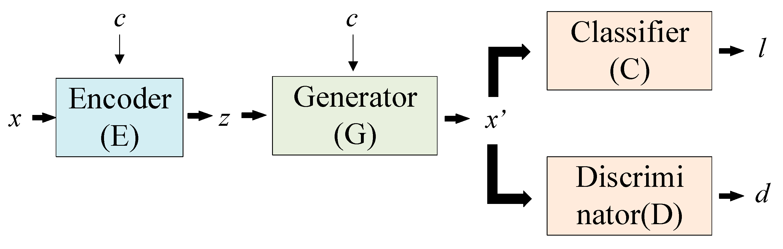
2.1. Conditional Variational Generative Adversarial Networks (CVAE-GAN)

The model structure is shown in Figure 1 and includes four parts: encoder network, E, generator network, G, discriminator network, D, and classifier network, C.
The encoder network, E, maps a sample, x, to a potential representation, z, via a learnable distribution, P(z|x,c), with c denoting the class of the data. Bounds on the prior P(z) and the recommended distribution are reduced using KL loss:
L K L = 1 2 ( log σ 2 + μ 2 + σ 2 1 )
where μ and σ are the mean and covariance of the output of the potential vector from encoder network E.
The generative network, G, generates the data, x′, by sampling from the learnable distribution, P(x′|z,c). The functions of G and D are the same as GAN. The network, G, attempts to learn the distribution of the real data by means of gradients from the discriminator network, D, which is able to distinguish between true/false samples. The loss function of the discriminator network, D, is:
L D = Ε x ~ p r [ log D ( x ) ] Ε z ~ p z [ log ( 1 D ( G ( z ) ) ) ]
where x is the input data and z is the potential vector from encoder network, E.
The generator uses an average feature matching the objective function. This objective function requires the feature centers of the synthetic samples to match the feature centers of the real samples. The generator, G, tries to minimize the loss function as:
L G D = 1 2 Ε x ~ p r f D ( x ) Ε z ~ p z f D ( G ( z ) ) 2 2
where fD(x) denotes the features in the middle layer of the discriminator, D.
The generating network, G, uses the average feature to match the objective function. Let the network, G, attempt to minimize:
L G C = 1 2 c Ε x ~ p r f C ( x ) Ε z ~ p z f C ( G ( z , c ) ) 2 2
where fC(x) denotes the intermediate layer outputs of the classifier and c denotes the label of the input data, x.
Then, an L2 reconstruction loss and pairwise feature matching-based loss are added to x and x′:
L G = 1 2 ( x x 2 2 + f D ( x ) f D ( x ) 2 2 + f C ( x ) f C ( x ) 2 2 )
where x is the input data and x′ is the generated data from the generator, G.
Network C takes x′ as input and outputs a k-dimensional vector, which is then converted to probability-like values using the softmax function. Each port of the output represents the posterior probability, P(c|x′). In the training phase, network, C, attempts to minimize the softmax loss. The function of the classifier network, C, is to measure the posterior of P(c|x′):
L C = Ε x ~ p r [ log P ( c x ) ]
The total loss function is:
L = L K L + L G + L G D + L G C + L D + L C
LKL is only relevant to the encoder network, E, indicating whether the distribution of potential vectors is as expected. LG, LGD, and LGC are relevant to the generator network, G, indicating whether the synthetic sample is the same as the input training samples, the real sample, and other samples in the same category, respectively. LC is relevant to the classifier network, C, indicating how well the network is used to classify different categories of samples; LD is relevant to the discriminator network, D, indicating how well the network is able to distinguish between real/synthetic samples. All these objective functions are complementary to each other and ultimately lead to optimal results for the algorithm.

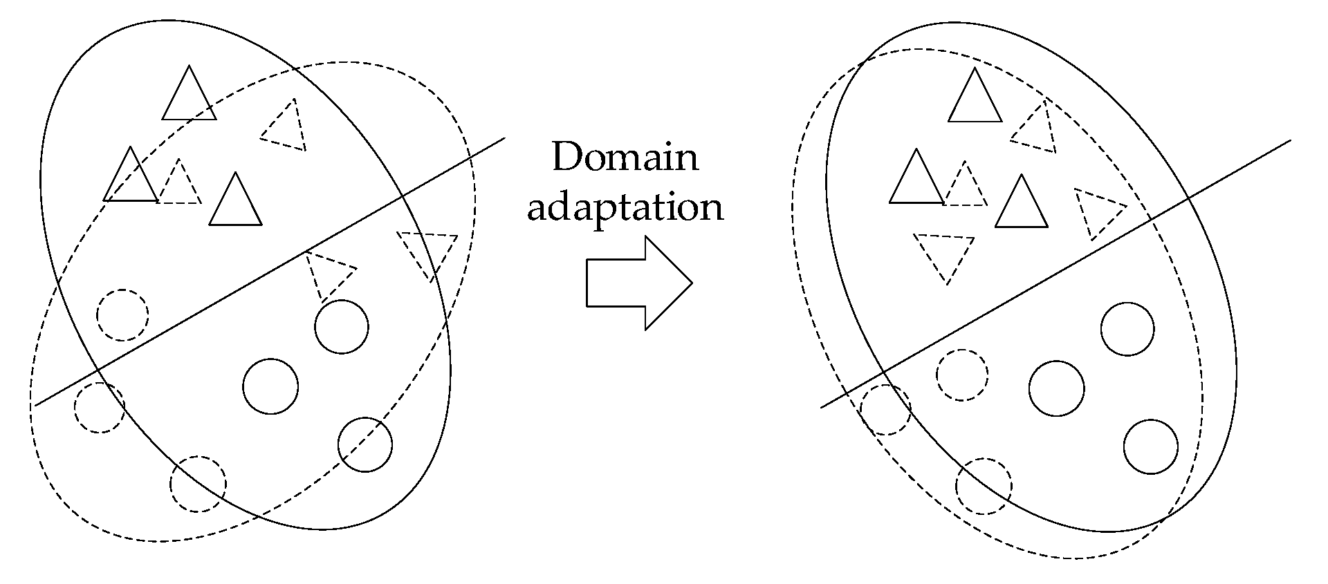
2.2. Domain Adaptive Technology (DA)

As shown in Figure 2, domain adaptation is used to map data features from different domains to the same feature space, so that other domain data can be used to enhance the target domain training. There are two fundamental concepts in domain adaptation: the source domain and the target domain. The source domain, DS = {XS, P(XS)}, is rich in supervised learning information. The target domain, DT = {XT, P(XT)}, represents the domain in which the test set is located, usually without labels or with only a few labels. Source and target domains are often the same type of task but are distributed differently.
Common domain adaptation methods include:
(1)
Sample adaptation: resampling samples in the source domain so that their distribution converges with the target domain distribution.
(2)
Feature adaptation: projecting the source and target domains into a common feature subspace.
(3)
Model adaption: modification of the source domain error function.
Domain loss is calculated using the maximum mean difference (MMD). To be specific, the transferable features are first mapped into reproduced kernel Hilbert space (RKHS), in which the mean distance between them is viewed as the metric to their distribution discrepancy:
M M D ( X S , X T ) = 1 X S ϕ ( x s ) 1 X T ϕ ( x t )
where ϕ is a mapping function, XS is the source data, and XT is the target data.

3. Transfer Learning Based on Conditional Variational Generative Adversarial Networks (TL-CVAE-GAN)

In this paper, we proposed a model named transfer learning based conditional variational generative adversarial networks (TL-CVAE-GAN) for fault diagnosis of wind turbine transmission platform datasets under different conditions. An improved CVAE-GAN is used for transfer learning to achieve the generation of unknown samples in different conditions.
As shown in Table 1, the data in this paper include XS1, XS2, XT1, and XT2. XS is the source domain data and XT is the target domain data. XS1 and XT1 are in operating speed 1, XS2 and XT2 are in operating speed 2. In this paper, XT2 is unknown.
The model structure of TL-CVAE-GAN is shown in Figure 3. A generative model CVAE-GAN1 is trained to generate XS2′ from XS1, and another generative model CVAE-GAN2 is trained to generate XT2′ from XT1. The structure of the neural network model is the same for CVAE-GAN1 and CVAE-GAN2, both containing: an encoder, E, a decoder, De, a generator, G, and a discriminator, D.
Assume that X1 is the data corresponding to Speed1 and X2 is the data corresponding to Speed2. The data, X1, is fed into the encoder, E, together with Speed1 for dimensionality reduction to obtain an intermediate code, z, with the Speed1 information removed; z is input to the decoder, De, for reconstruction, and the mean, u, and variance, σ, are additionally obtained from z. The variance, σ, is multiplied by the random noise, e, plus the mean, u, to obtain zs; zs is fed into the generator, G, together with Speed2 to produce X2′. The real X2 is fed into the discriminator, D, together with the generated X2′ for discrimination. The accuracy of the generated model is improved by confronting the generator with the discriminator.
The MMD of XS1 to XT1 is solved for domain adaptation. The MMD is added to the loss function of the generator CVAE-GAN2 for backpropagation to generate XT2′.
The TL-CVAE-GAN model is divided into the following steps:
In the first step, update the parameters of CVAE-GAN1 and generate XS2′. The source data XS1 and its corresponding rotational speed are input into encoder E to obtain the intermediate key feature, z, with the rotational speed information removed. The mean value, u, and variance, σ, are obtained from z, then a new sample, zs, is formed by u, σ, and the noise e; z is fed into the decoder De for reconstruction and zs and the corresponding speed, speed2, are input to the generator, G, to generate XS2′. The discriminator, D, discriminates between the generated data, XS2′, and the real data, XS2. The loss of CVAE-GAN1 is:
L o s s 1 = L o s s V A E + L o s s G A N
L o s s V A E = X S 1 X S 1 2 2 + 1 2 ( log σ 2 + μ 2 + σ 2 1 )
L o s s G A N = Ε x ~ p r [ log D ( X S 2 ) ] Ε z ~ p z [ log ( 1 D ( G ( z s , s p e e d 2 ) ) ) ]
where XS1 is the input source data, XS1′ is the generated data from XS1, μ and σ are the mean and covariance of the output of the potential vector from the encoder network, E, XS2 is another input source data that the operating conditions are different from XS1, speed2 is the operating speed of XS2, and zs is the potential vector of source data from encoder network, E.
In the second step, update the parameters of CVAE-GAN2. The MMD between CVAE-GAN1 and CVAE-GAN2 is calculated. The MMD is added to the loss of CVAE-GAN2 to achieve the generator’s domain migration. The loss is as follows:
L o s s 2 = M M D ( X S 1 , X T 1 ) + M M D ( z s , z t ) + M M D ( X S 2 , X T 2 ) + M M D ( f D ( X S 2 ) , f D ( X T 2 ) )
where fD(x) denotes the features in the penultimate layer of the discriminator, D. XT1 and XT2 are the target data and zs and zt are the potential vector of source data and target data from encoder network E.
In the last step, repeat steps 1 and steps 2 for 5 training cycles to generate the unknown data, XT2′.
The model structure of the classifier is shown in Figure 4. The existing data, XS1, XS2, XT1, and the generated data, XT2′, are together input into the classifier for training.
The classifier model contains three convolution layers, three BatchNorm1d, three MaxPool1d, and one fully-connected layer. The number of neurons in each layer is shown in Figure 4. The activation function for the last layer is Softmax and the activation functions for the other layers are Relu. All the data goes through the fast Fourier transform, and is then fed into the model. The classifier is updated by:
L o s s 21 = x i , y i ~ T i [ y i log y i + ( 1 y i ) log ( 1 y i ) ]
where yi is the real label of the data and yi’ is the output of the classifier model.
The feature embedding is visualized by t-SNE to test the effectiveness of the proposed model. The complete algorithm flow is shown in Algorithm 1.
Algorithm 1. TL-CVAE-GAN
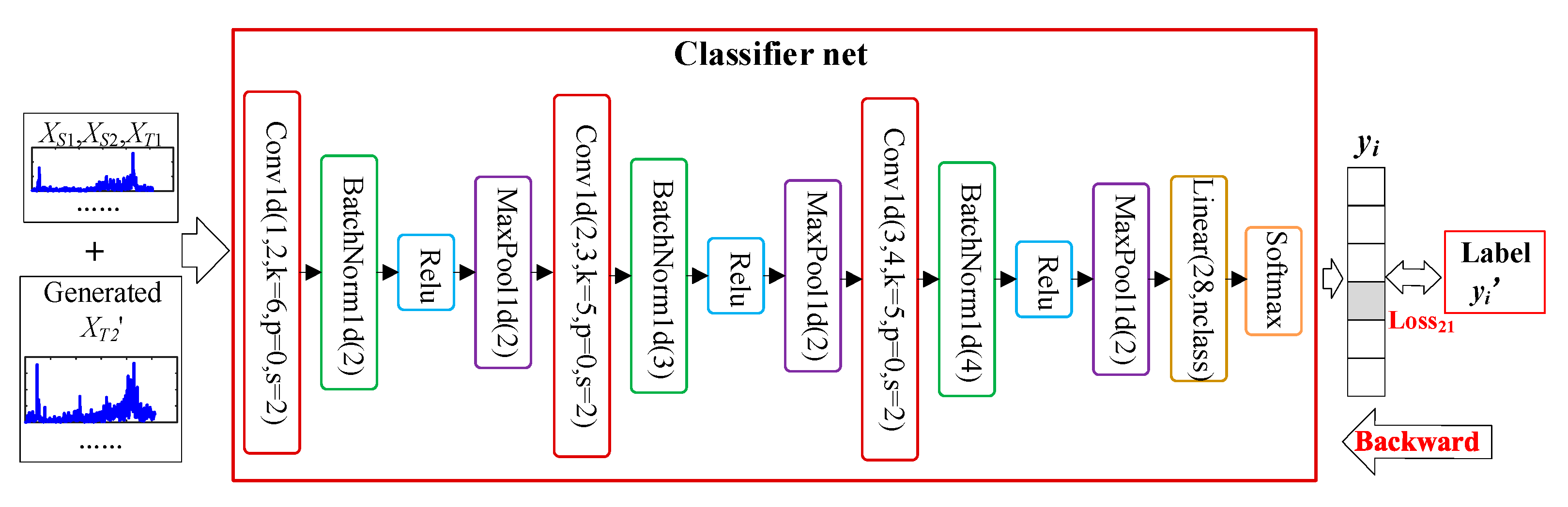
Input: Input training data, T r = X S 1 , Y S 1 , X S 2 , Y S 2 , X T 1 , Y T 1 , testing data, T e , classified model, fC. In the CVAE-GAN1 model: encoder network, fE1, decoder network, fDE1, generator network, fG1, and discriminator network, fD1. In the CVAE-GAN2 model: encoder network, fE2, generator network, fG2, discriminator network, fD2.The learning rate, lr.
########################Cycle 5 times ####################
1: For f from 0 to 4:
########################train CVAE-GAN1 model ####################
2:      For each training epoch, do:
3:         For each batch, do:
4:           zi = fE1(xs1i, Speed1), xs1i’ = fDE1(zi), the mean value, usi, and variance, σsi, are obtained from zi, sample e from the random noise S. zsi = usi +σsi *e,
xs2i’= fG1(zsi, Speed2), ds2i’= fD1(xs2i’), ds2i= fD1(xs2i)
5:         Backward propagation by Equation (9).
6:       end
7:       save CVAE-GAN1 model
#################### train CVAE-GAN2 model use MMD #######################
8:       download CVAE-GAN1 model. Use the parameters of the CVAE-GAN1 model as the initial parameters of CVAE-GAN2.
9:       For each training, do:
10:         For each batch, do:
11:           zi = fE2(xt1i), zti = uti +σti *e, xt2i’= fG2(zti),
12:        Backward propagation by Equation (12).
13:       end
14:       save CVAE-GAN2 model
15:       lr = lr/2
16:       if f > 0:
17:         download the CVAE-GAN2 model. Use the parameters of the CVAE-GAN2 model as the initial parameters of CVAE-GAN1.
18: end
########### train classifier net use Tr and the generate data XT2′ #################
########the input data is X = {(XS1, YS1), (XS2, YS2), (XT1, YT1), (XT2′, YT2)}###########
19: For each training, do:
20:       For each batch, do:
21:         yi’ = fC(xi)
22:       Backward propagation by Equation (13).
23: end
###################### testing results and t-SNE #########################
24: For the test set, calculate cTi = fC (Tei), calculate the accuracy, and draw the t-SNE diagram.
Output: testing results.

4. Case Analysis

In this section, the data of the wind turbine transmission platform are used to verify our model. The wind turbine transmission platform is shown in Figure 5. It consists of a drive motor, a stator gearbox, a planetary gearbox, and a load device to simulate the vibration state under various gear faults.
The number of teeth of each gear in the drive system is shown in Figure 6. The stator gearbox consists of four gears in a two-stage drive with three shafts. The fault occurred in the intermediate shaft gear. Piezoelectric sensors are placed on the bearing seat at the right end of the intermediate shaft. This paper simulates the multiple faults of a wind turbine gearbox under variable operating conditions. Six fault modes in the stator gearbox are adopted, including normal, cracked, chipped, missing teeth, wear, and eccentricity. The data available is shown in Table 2. The data consists of six categories, with one health category and five fault categories. The first three categories contain data for four operating speeds (38 Hz, 40 Hz, 43 Hz, 45 Hz) and the last three categories only have data for 43 Hz and 45 Hz. The speed is of the driver motor. The data is sampled at a frequency of 8192 Hz; 256 data are available in each category for each working condition.
The data description of the training dataset and testing dataset is shown in Table 3. There are 256 data in each category for each speed. For each class of data under each speed, the first 160 are taken as the training set and all data are testing data. The trained percentages are 62.5%. This case addresses the problem of unbalanced data from the wind turbine transmission platform, generating missing data and improving diagnostic accuracy. Therefore, in this case, the data in categories 3, 4, and 5 where the speed is 38 Hz and 40 Hz are set missing and are not included in the training set.
For the TL-CVAE-GAN and classifier model, the update function is Adam, the training epochs for the update are 400, and the batch size is 32.
Figure 7, Figure 8 and Figure 9 show the missing data, XT2′, generated by the generator CVAE-GAN2. It can be seen that the generator effectively generates data for the unknown operating conditions (38 Hz, 40 Hz).
In this case, it is the pinion of the intermediate shaft that has failed. Therefore, the rotational frequency is given in Equation (14) and the meshing frequency is given in Equation (15).
f r = s p e e d × 29 / 100
f m = f r × 36
When the operating condition is 38 Hz, the rotational frequency is 397 Hz and the meshing frequency is 11 Hz. When the operating condition is 40 Hz, the rotational frequency is 418 Hz and the meshing frequency is 12 Hz. The rotational and meshing frequency characteristics are evident in both the real data and the generated data. At the same time, there are differences in the frequency spectrum of missing, wear, and eccentric faults.
Figure 7 shows a missing fault. When a gear has a broken tooth, there is a strong shock at the broken tooth for every week the gear rotates, so there are distinct rotational and meshing frequencies present in the frequency spectrum. It is clearly modulated by the rotational frequency throughout the frequency band. The edge band is characterized by a large number of edge frequencies, a wide range, and a uniform and relatively flat distribution. It can be seen that the generated data effectively exhibits these characteristics.
Figure 8 shows a wear fault. The gears are uniformly worn, with a high amplitude sideband at the engagement frequency and its harmonics. The amplitude of the higher harmonics of the meshing frequency is large. In this data, the wear is more severe and the amplitude of the second harmonic has exceeded the amplitude of the fundamental wave of the meshing frequency. It can be seen that the generated data effectively exhibits these characteristics.
Figure 9 shows an eccentric fault. This data has only eccentricity, no faulty gears, so there are no sidebands at the meshing frequency. It can be seen that the generated data effectively exhibits these characteristics.
The generated data for the unknown working conditions are trained together with the known data for the classifier. We compared the classification accuracy of the trained model using only the training set and the training set with the generated unknown data. For better comparison, the same classifier, the same number of training epochs, and the same learning rate were used for both cases. The obtained fault classification accuracy and t-SNE is shown in Figure 10. The comparison of classification accuracy with and without the addition of generated data is shown in Table 4. It can be seen that after the data generated by TL-CVAE-GAN with unknown working conditions were added to the training set, the test accuracy of the trained classifier was improved by 21.3%.

5. Conclusions

Fault diagnosis of wind turbines plays an important role in improving the reliability of wind turbines. However, the operating conditions of wind turbines vary randomly, and data on different operating conditions are not easily available.
In this paper, the wind turbine transmission platform data is supplemented by the generation of data for unknown operating conditions, which in turn improves the classification accuracy. The proposed TL-CVAE-GAN model combines the better performance of CVAE-GAN in generating samples with the idea of domain adaptive migration. It achieves the generation of unknown samples for wind turbine transmission platforms in different conditions and solves the classification problem of variable conditions data. Work conditions are input to the model as conditions, and the generation of data in different work conditions between similar classes is achieved by domain migration. The known data are used to train CVAE-GAN1. In CVAE-GAN, the known working conditions are fed into the encoder as conditional information to obtain the intermediate key information for the removal of the working conditions. The intermediate key information and the unknown conditions are fed together into the generator to generate the same class of data for the unknown conditions. The generation can be improved by confronting the generator with the discriminator.
The MMD between the known and unknown conditions is then calculated. The MMD is added to the loss of CVAE-GAN2, which is an unknown generator, to achieve the generator’s domain migration. The problem of data imbalance for wind turbine gearboxes is solved by generating missing data for unknown working conditions via CVAE-GAN2. The raw data and generated data are fed into the classifier to train the model for classification.
The results show that the proposed model, TL-CVAE-GAN, effectively generates data for unknown working conditions. After the generated data of unknown operating conditions were added to the training set as a supplement, the test accuracy of the trained classifier was improved by 21.3%, effectively improving the fault diagnosis accuracy under-sample imbalance. The model can better solve the problem of fault diagnosis of wind turbines with variable operating conditions.

Author Contributions

Writing—original draft, X.L.; Writing—review & editing, H.M. and Y.L. All authors have read and agreed to the published version of the manuscript.

Funding

This research received no external funding.

Informed Consent Statement

Informed consent was obtained from all subjects involved in the study.

Conflicts of Interest

The authors declare no conflict of interest.

References

  1. Li, W.; Chen, Z.; He, G. A novel weighted adversarial transfer network for partial domain fault diagnosis of machinery. IEEE Trans. Ind. Inform. 2020, 17, 1753–1762. [Google Scholar] [CrossRef]
  2. Huang, R.; Li, J.; Liao, Y.; Chen, J.; Wang, Z.; Liu, W. Deep adversarial capsule network for compound fault diagnosis of machinery toward multidomain generalization Task. IEEE Trans. Instrum. Meas. 2020, 70, 3506311. [Google Scholar] [CrossRef]
  3. Li, J.; Huang, R.; He, G.; Liao, Y.; Wang, Z.; Li, W. A two-stage transfer adversarial network for intelligent fault diagnosis of rotating machinery with multiple new faults. IEEE ASME Trans. Mechatron. 2020, 26, 1591–1601. [Google Scholar] [CrossRef]
  4. Chen, Z.; Gryllias, K.; Li, W. Intelligent fault diagnosis for rotary machinery using transferable convolutional neural network. IEEE Trans. Ind. Inform. 2020, 16, 339–349. [Google Scholar] [CrossRef]
  5. Li, J.; Huang, R.; He, G.; Wang, S.; Li, G.; Li, W. A deep adversarial transfer learning network for machinery emerging fault detection. IEEE Sens. J. 2020, 20, 8413–8422. [Google Scholar] [CrossRef]
  6. Li, S.; An, Z.; Lu, J. A novel data-driven fault feature separation method and its application on intelligent fault diagnosis under variable working conditions. IEEE Access 2020, 8, 113702–113712. [Google Scholar] [CrossRef]
  7. Qian, W.; Li, S.; Yi, P.; Zhang, K. A novel transfer learning method for robust fault diagnosis of rotating machines under variable working conditions. Measurement 2019, 138, 514–525. [Google Scholar] [CrossRef]
  8. Guo, L.; Lei, Y.; Xing, S.; Yan, T.; Li, N. Deep convolutional transfer learning network: A new method for intelligent fault diagnosis of machines with unlabeled data. IEEE Trans. Ind. Electron. 2019, 66, 7316–7325. [Google Scholar] [CrossRef]
  9. Yang, B.; Lei, Y.; Jia, F.; Xing, S. An intelligent fault diagnosis approach based on transfer learning from laboratory bearings to locomotive bearings. Mech. Syst. Signal Process. 2019, 122, 692–706. [Google Scholar] [CrossRef]
  10. Gretton, A.; Borgwardt, K.M.; Rasch, M.J.; Schölkopf, B.; Smola, A. A kernel two-sample test. Mach. Learn. Res. 2012, 13, 723–773. [Google Scholar]
  11. Venkateswara, H.; Chakraborty, S.; Panchanathan, S. Deep-learning systems for domain adaptation in computer vision learning transferable feature representations. IEEE Signal Process. 2017, 34, 117–129. [Google Scholar] [CrossRef]
  12. Sun, S.; Zhang, B.; Xie, L.; Zhang, Y. An unsupervised deep domain adaptation approach for robust speech recognition. Neurocomputing 2017, 257, 79–87. [Google Scholar] [CrossRef]
  13. Zhang, Z.; Chen, H.; Li, S.; An, Z. Unsupervised domain adaptation via enhanced transfer joint matching for bearing fault diagnosis. Measurement 2020, 165, 108071. [Google Scholar] [CrossRef]
  14. Zhang, Z.; Chen, H.; Li, S.; An, Z.; Wang, J. A novel geodesic flow kernel based domain adaptation approach for intelligent fault diagnosis under varying working conditions. Neurocomputing 2019, 376, 54–64. [Google Scholar] [CrossRef]
  15. An, Z.; Li, S.; Jiang, X.; Xin, Y.; Wang, J. Adaptive cross-domain feature extraction method and its application on machinery intelligent fault diagnosis under different working conditions. IEEE Access 2019, 8, 535–546. [Google Scholar] [CrossRef]
  16. Qian, W.; Li, S.; Jiang, X. Deep transfer network for rotating machine fault analysis. Pattern Recognit. 2019, 96, 106993. [Google Scholar] [CrossRef]
  17. Yang, B.; Lei, Y.; Jia, F.; Li, N.; Du, Z. A polynomial kernel induced distance metric to improve deep transfer learning for fault diagnosis of machines. IEEE Trans. Ind. Electron. 2019, 67, 9747–9757. [Google Scholar] [CrossRef]
  18. Goodfellow, I.J.; Pouget-Abadie, J.; Mirza, M.; Xu, B. Generative adversarial nets. In Proceedings of the International Conference on Neural Information Processing Systems, Montreal, QC, Canada, 8–13 December 2014; pp. 1–9. [Google Scholar]
  19. Zheng, T.; Song, L.; Wang, J.; Teng, W.; Xu, X. Data synthesis using dual discriminator conditional generative adversarial networks for imbalanced fault diagnosis of rolling bearings. Measurement 2020, 158, 107741. [Google Scholar] [CrossRef]
  20. Wang, J.; Li, S.; Han, B.; An, Z.; Bao, H.; Ji, S. Generalization of deep neural networks for imbalanced fault classification of machinery using generative adversarial networks. IEEE Access 2019, 7, 111168–111180. [Google Scholar] [CrossRef]
  21. Schlegl, T.; Seebck, P.; Waldstein, S.M.; Schmidt-Erfurth, U.; Langs, G. Unsupervised anomaly detection with generative adversarial networks to guide marker discovery. Comput. Vis. Pattern Recognit. 2017, 10265, 146–157. [Google Scholar]
  22. Akcay, S.; Atapour-Abarghouei, A.; Breckon, T.P. GANomaly: Semi-supervised anomaly detection via adversarial training. Comput. Vis. Pattern Recognit. 2018, 11363, 622–637. [Google Scholar]
  23. Guo, Q.; Li, Y.; Song, Y.; Wang, D.; Chen, W. Intelligent fault diagnosis method based on full 1-D convolutional generative adversarial network. IEEE Trans. Ind. Inform. 2019, 16, 2044–2053. [Google Scholar] [CrossRef]
  24. Lyu, Y.; Han, Z.; Zhong, J.; Li, C.; Liu, Z. A generic anomaly detection of catenary support components based on generative adversarial networks. IEEE Trans. Instrum. Meas. 2020, 69, 2439–2448. [Google Scholar] [CrossRef]
  25. Yan, K.; Su, J.; Huang, J.; Mo, Y. Chiller fault diagnosis based on VAE-enabled generative adversarial networks. IEEE Trans. Autom. Sci. Eng. 2020, 19, 387–395. [Google Scholar] [CrossRef]
  26. Liu, S.; Jiang, H.; Wu, Z.; Li, X. Data synthesis using deep feature enhanced generative adversarial networks for rolling bearing imbalanced fault diagnosis. Mech. Syst. Signal Process. 2022, 163, 108139. [Google Scholar] [CrossRef]
  27. Kingma, D.P.; Welling, M. Auto-encoding variational bayes. arXiv 2014, arXiv:1312.6114. [Google Scholar]
  28. Makhzani, A.; Shlens, J.; Jaitly, N.; Goodfellow, I.; Frey, B. Adversarial autoencoders. arXiv 2015, arXiv:1511.05644. [Google Scholar]
  29. Qu, F.; Liu, J.; Ma, Y.; Zang, D.; Fu, M. A novel wind turbine data imputation method with multiple optimizations based on GANs. Mech. Syst. Signal Process. 2020, 139, 106610. [Google Scholar] [CrossRef]
  30. Guo, Z.; Pu, Z.; Du, W.; Wang, H.; Li, C. Improved adversarial learning for fault feature generation of wind turbine gearbox. Renew. Energy 2022, 185, 255–266. [Google Scholar] [CrossRef]
  31. Jiang, N.; Li, N. A wind turbine frequent principal fault detection and localization approach with imbalanced data using an improved synthetic oversampling technique. Int. J. Electr. Power Energy Syst. 2021, 126, 106595. [Google Scholar] [CrossRef]
  32. Jing, B.; Pei, Y.; Qian, Z.; Wang, A.; Zhu, S.; An, J. Missing wind speed data reconstruction with improved context encoder network. Energy Rep. 2022, 8, 3386–3394. [Google Scholar] [CrossRef]
  33. Wang, A.; Qian, Z.; Pei, Y.; Jing, B. A de-ambiguous condition monitoring scheme for wind turbines using least squares generative adversarial networks. Renew. Energy 2022, 185, 267–279. [Google Scholar] [CrossRef]
  34. Yu, X.; Zhang, X.; Cao, Y.; Xia, M. VAEGAN: A collaborative filtering framework based on adversarial variational autoencoders. In Proceedings of the Twenty-Eighth International Joint Conference on Artificial Intelligence (IJCAI-19), Macao, China, 10–16 August 2019; pp. 4206–4212. [Google Scholar]
  35. Bao, J.; Chen, D.; Wen, F.; Li, H.; Hua, G. CVAE-GAN: Fine-grained image generation through asymmetric training. In Proceedings of the IEEE International Conference on Computer Vision (ICCV), Venice, Italy, 22–29 October 2017; pp. 2745–2754. [Google Scholar]
Figure 1. Model structure of CVAE-GAN.
Sustainability 14 05441 g001
Figure 2. Domain adaptation.
Sustainability 14 05441 g002
Figure 3. Model structure of TL-CVAE-GAN.
Sustainability 14 05441 g003
Figure 4. Model structure of the classifier.
Sustainability 14 05441 g004
Figure 5. Transmission platform of wind turbine.
Sustainability 14 05441 g005
Figure 6. General structure of the gear system.
Sustainability 14 05441 g006
Figure 7. The generated data and its corresponding real data for fault 3 at 38 Hz and 40 Hz.
Sustainability 14 05441 g007
Figure 8. The generated data and its corresponding real data for fault 4 at 38 Hz and 40 Hz.
Sustainability 14 05441 g008aSustainability 14 05441 g008b
Figure 9. The generated data and its corresponding real data for fault 5 at 38 Hz and 40 Hz.
Sustainability 14 05441 g009
Figure 10. The t-SNE of the classify using only the training set and the training set with the generated unknown data.
Sustainability 14 05441 g010
Table 1. Variables and conditions of the data.
DomainDataWork ConditionKnown or Not
Source domainXS1Speed1Data available
XS2Speed2Data available
Target domainXT1Speed1Data available
XT2Speed2Data not available
Table 2. Fault description of wind turbine transmission platform.
Fault ModesLabelSpeed (Hz)Sampling FrequencyNumber of Dataset
Normal038, 40, 43, 458192 Hz256 × 4
Cracked138, 40, 43, 458192 Hz256 × 4
Chipped238, 40, 43, 458192 Hz256 × 4
Missing343, 458192 Hz256 × 2
Wear443, 458192 Hz256 × 2
Eccentricity543, 458192 Hz256 × 2
Table 3. Data description of the training dataset and testing dataset.
DataLabelSpeed (Hz)Number of Training DatasetNumber of Testing Dataset
Source domainXS10, 1, 243, 45160 × 3 × 2256 × 3 × 2
XS20, 1, 238, 40160 × 3 × 2256 × 3 × 2
Target domainXT13, 4, 543, 45160 × 3 × 2256 × 3 × 2
XT23, 4, 538, 400256 × 3 × 2
Table 4. Comparison of classification accuracy with and without the addition of generated data.
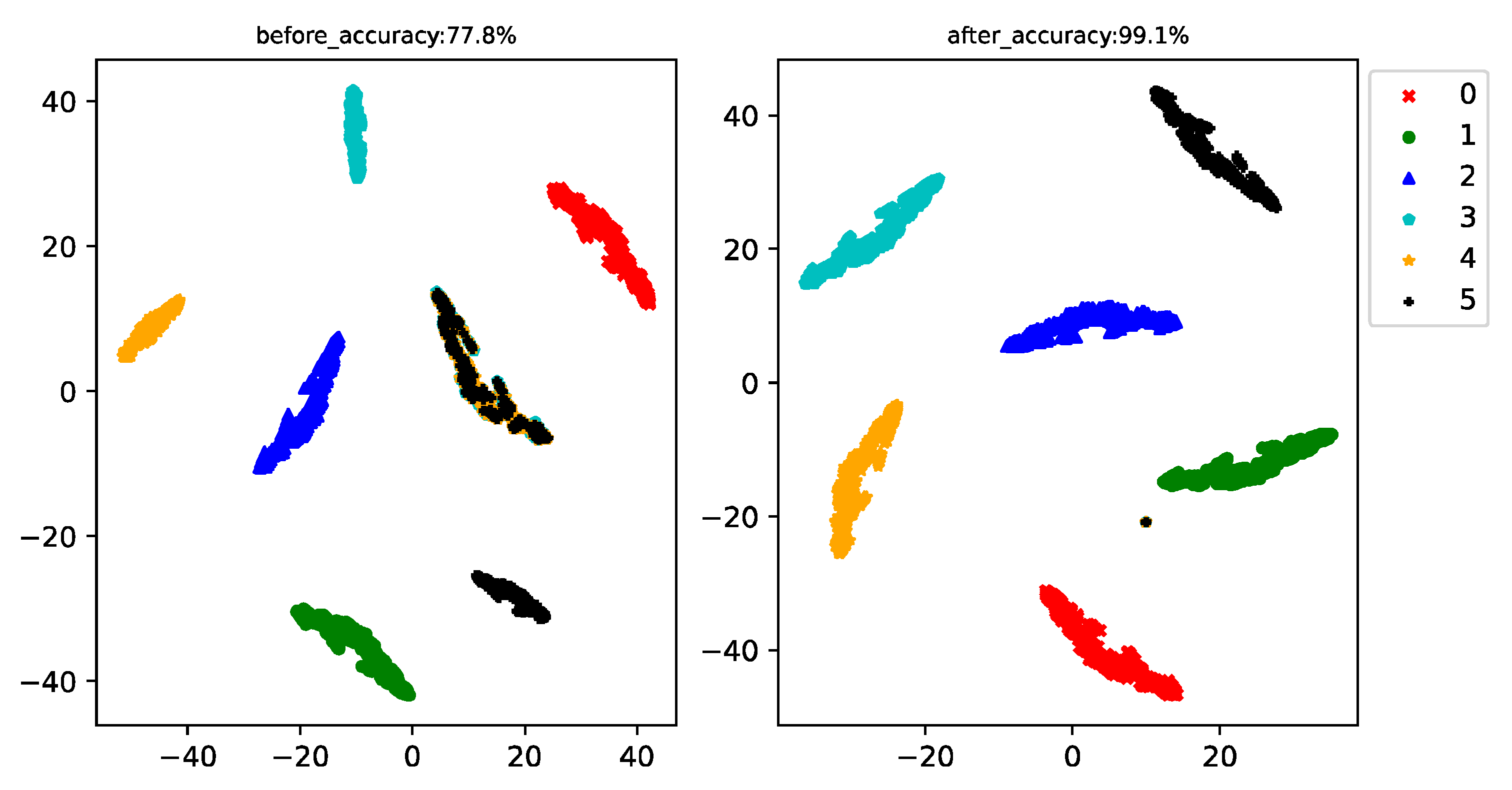
Only the Training Set Trains the ClassifierTraining Set and Generated Data together to Train the ClassifierImproved
Classification accuracy77.8%99.1%21.3%
Publisher’s Note: MDPI stays neutral with regard to jurisdictional claims in published maps and institutional affiliations.

