How to Reduce Individuals’ Ecological Footprint without Harming Their Well-Being: An Application to Belgium

Abstract

Human activities are a key driver of many environmental problems the world is facing today, including climate change, the disruption of biogeochemical cycles, and biodiversity loss. Behavioural changes at the individual and household level are needed to reduce humanity’s environmental impact, but people also need the capacity to behave in a sustainable way. If their well-being is negatively impacted or if behaving sustainably is too time consuming or too expensive, people might be less inclined to change their behaviour. In this article, we look at the determinants of different types of pro-environmental behaviour and how these are associated with their experienced levels of well-being. More specifically, we focus on the determinants of behaviours that influence both the ecological footprint (EF) and satisfaction with life. In our analysis we include socio-demographic characteristics and a number of psychological antecedents of pro-environmental behaviour (PEB). The data we use was collected in Flanders (Belgium) and allows us to calculate the EF of each respondent individually. Our main conclusions are threefold. First, even if individuals are provided with opportunities to behave in a more sustainable way, they do not always do so (e.g., richer people on average have a higher EF). Efforts could be put in place at the collective side (e.g., public infrastructure) to stimulate people to reduce their environmental impact. Second, as we distinguish seven EF components, we are able to show differential effects of each of the determinants. Third, the association between PEB and satisfaction with life is not strong: only the type of housing is significantly associated with satisfaction with life. Related to that, the psychological antecedents of PEB are only associated with the EF, not with satisfaction with life.

1. Introduction

Human activities have huge and rising impacts on the environment and the climate. Rockström (2009) [1] argues that three planetary boundaries have already been transgressed: climate change, biodiversity loss, and changes to the global nitrogen cycle. Many warn that future environmental conditions will be far more dangerous than currently believed (see [2]). We need to produce, sell, buy, use, and consume less material goods, use less space, and emit less. Changes towards a less environmentally impactful lifestyle are needed in order to reduce the human impact on the ecosystem, especially in developed countries. Measuring the human impact on ecological systems or on nature is complicated due to the fact that there are many ecological dimensions involved: renewable and non-renewable resource use, CO${}_2$ emissions, environmental degradation, plastic use, land use, and so on. Comparing the environmental benefits of turning vegan to those of adopting slow mobility is not easy, as several different dimensions are involved. An overarching one-dimensional way to measure the ecological impact of individual behaviour is the ecological footprint (EF) [3]. The EF is a measure of human demand for the biologically productive land (expressed in a land area called ‘global hectares’ (gha)) that is needed to provide a given population with the biotic resources it consumes and to absorb the CO${}_2$ emissions that it generates. Hence, the environmental impacts of different components (energy use, food, mobility, etc.) are aggregated into a single number that can be compared to the biocapacity available to the population under consideration. At present, the average available biocapacity on Earth is around two global hectares per person, so in order to live in balance with nature, an individual’s ecological footprint should be smaller than that.

In the last decade, the per capita ecological footprint has increased worldwide. According to the WWF, humanity is currently using 1.5 Earths on a yearly basis, that is, the demand for biocapacity is 50% higher than its supply [4], and the overshoot is increasing. The ecological overshoot in developed countries is much higher. For instance, if everyone on Earth adopted the lifestyle of an average Western European, four planets would be needed. The advantage of the EF is that it can be calculated on several levels: for groups of people (national, regional) or at the individual level. In order to tackle the aforementioned challenges, many countries have agreed to reduce carbon dioxide emissions (e.g., via the Paris Agreement) and other environmental impacts. However, it should be noted that many of these countries are having difficulties reaching the goals set [2,5].

An individual’s ecological footprint is the sum of the individual’s demands for biocapacity (gha) due to his or her behaviours related to several footprint components (mobility footprint, housing footprint, food footprint, energy use footprint, etc.). To decrease the ecological footprint, individual behavioural changes related to these different components are often called for [6,7]. Pro-environmental behaviour (PEB) means that the individual takes action related to one (or more) of these behaviours in order to avoid harm to the environment and/or safeguard the environment [8]. Changing these behaviours is complex, and typically, many drivers are involved [9], which are both exogenous and endogenous to the individual. The literature on pro-environmental behaviour scrutinize the impact of both exogenous and endogenous factors at play in these decisions. This article aims to understand the determinants of PEB for each of the EF components, and for the total EF at the individual level.

In order to do that, we will first develop a micro-economic model of individual choices, which leads to experiences of individual well-being. In this model, we will incorporate other determinants from the literature on PEB: socio-demographic characteristics and psychological antecedents of PEB. From a micro-economic perspective, individuals face several constraints (e.g., time constraints [9,10] and budget constraints [8,11,12]): each of the choices entails a time cost and a monetary cost [13]. Both the budget or income constraint and the time constraint limit the feasible options. For instance, going to work by train may take more time than driving by car, and consuming organic food might be more expensive than non-organic food. At the same time, these constraints depend on the individual’s life circumstances: for someone living in the city, public transport is less time consuming (relative to driving a car) than for someone living on the countryside, who has less access to public transport. Someone with young children might not have options other than taking the car for bringing children to school and arriving at work on time. This kind of reasoning is in line with Steg and Vlek (2009) [8], who identify perceived costs and benefits as an important determinant of pro-environmental behaviour in their review paper, while Ferrara and Missios (2005) [12] show that increasing the user fees for garbage collection has a positive influence on recycling behaviour, though other measures entice less behavioural change.

At the moment of the decision, the household makes choices in order to maximise their decision utility. Decision utility is a representation of the individuals’ preferences at the moment of choice [14,15]. Preferences here simply refer to the trade-offs that people make, which can depend on socio-demographic characteristics (e.g., age) or on specific psychological antecedents (e.g., environmental concern), which we study below. Consequently, individuals facing the same constraints might behave differently: some will act in a more environmentally friendly way than others. Importantly, many have argued that there is a difference between decision utility and experienced utility. While decision utility reflects preferences at the moment of decision making, experienced utility is the individual’s judgment about her or his hedonic experience [14,16]. At the moment of the decision, the individual uses his or her decision utility to judge the combination of behaviours, but when asked to evaluate this life situation, other elements can enter. The individual might regret certain choices, or might have suffered imperfect foresight. A choice might have been optimal at a certain moment in the individual’s life, but as time has passed, the individual looks at it very differently. At a certain moment in his or her life, an individual might have chosen to live on the countryside (e.g., to raise children in a calm, safe and green environment). Years later, the individual might evaluate his or her life situation very differently. In this study, we use satisfaction with life as an approximation of experienced utility.

The relation between pro-environmental behaviour (PEB) and satisfaction with life has been studied by several authors [17,18], and pro-environmental preferences may play a role in the decision-making process. If behavioural changes aimed at reducing environmental impacts are negatively associated with one’s individual satisfaction with life, individuals might be inclined to stick to the status quo. The literature provides mixed evidence, and concludes that it is a complex relation that can be positive, negative, or neutral [17,19,20]. Welsch and Kühling (2011) [17] arrive at a positive association between environmentally friendly consumption and life satisfaction, and Schmitt et al. (2018) [13] show that more frequently acting in a pro-environmental way leads to higher life satisfaction, but the association was stronger for behaviours that involved more social interaction, behaviours that were more easily observed, and behaviours that involved direct costs in terms of money, time, and effort [13]. Similarly, Binder and Blankenberg (2017) [21] find a positive relation, but argue that the positive influence on satisfaction with life has more to do with self-image than with actual pro-environmental behaviour. On the other hand, Andersson et al. (2014) [22], Verhofstadt et al. (2016) [23], and Herziger et al. (2020) [19] found no relation between satisfaction with life and pro-environmental behaviour. Verhofstadt et al. (2016) [23] also find that some components of the ecological footprint have a positive or negative association with satisfaction with life. For instance, having a relationship (living together) or owning a house both lead to higher satisfaction with life and a lower ecological footprint; living in rural areas or having a higher income increases the ecological footprint, while there is no influence on satisfaction with life. Finally, some studies also find a positive association between well-being or satisfaction with life and ecological footprint (e.g., [24]), suggesting that reducing the ecological footprint might lead to lower well-being. The positive association in [24] disappears, however, when income is incorporated as a control variable.

We have argued above that both the constraints and the preferences from the micro-economic model depend on several other factors; to these factors we turn now, as determinants of PEB. In their literature overview, Blankenberg and Alhusen (2018) [9] distinguish socio-demographic variables, psychological variables, habits, and contextual factors as determinants of pro-environmental behaviour. Other literature overviews can be found in Gifford and Nilsson (2014) [25] or Li et al. (2019) [26], who only distinguish between external (socio-demographic) and internal (psychological) factors. It is important to note that the focus in the literature is on the determinants of specific behaviours (e.g., recycling or energy use), not on an indicator encompassing all aspects of behaviour, as we study in this article.

The relation between different socio-demographic variables and PEB has been studied by several fields: social and environmental psychology, economics, education science, environmental studies, and so on. We provide a short overview of the determinants that are also used in our empirical analysis below. PEB is associated negatively with age [9], although older studies report a positive association [27]. Gifford and Nilsson (2014) [25] argue that the effect of age is simply due to a cohort effect and depends on experiences at various moments in a person’s life. The evidence on the relation between income and PEB is mixed, as a higher income provides opportunities to invest more in home insulation and energy-efficient appliances, but it also increases one’s total consumption level (often also including travel). Income increases environmental concern [28], but this is not always translated into behaviour. Büchs and Schnepf (2013) [6] report a positive association between income and PEB, while other authors report negative or no association between both variables (e.g., Whitmarsh and O’Neill, 2010 [29]). Education is positively associated with PEB, but more so for some types of behaviour (e.g., paper recycling, water use) than for others (travelling, house size) [9,30].

In their overview, Gifford and Nilsson (2014) [25] also pay attention to the individuals’ place of residence. People living in rural areas are living closer to nature than those living in urban areas, but the former might need a car more often than the latter. Gender plays a role in determining PEB, as women typically engage in more pro-environmental behaviours than men [9,25]. They are found to have lower EFs, for example, in terms of recycling, food uptake, and meat consumption. Family size is generally negatively associated with PEB and with environmental attitudes [31], although there is also a positive association with some PEBs (e.g., recycling). Larger families experience more time constraints (e.g., due to childcare, and budget constraints), and so have less opportunity to behave in a pro-environmental way. At the same time, sharing a house with family members reduces the environmental impact per household member, as a.o. heating is shared among members. Finally, the role of political orientation (ideology, partisanship) has been studied as well. We distinguish the individuals’ ethical position (ethically conservative versus liberal) and their economic position (economically liberal versus socialist). Those who are more people-oriented, who are less authoritarian, and who have higher post-materialist values, have higher levels of environmental concern and attitude [25]. Fransson and Gärling (1999) [28] conclude that, in the US, liberals are more environmentally concerned than conservatives, but the differences have become smaller with time.

The psychological antecedents of pro-environmental behaviour are analysed next. The literature reviews of Gifford and Nilsson (2014) [25], Blankenberg and Alhusen (2018) [9], and Li et al. (2019) [26] distinguish several psychological antecedents of PEB: beliefs, attitudes, awareness, values, (social) norms (e.g., biospheric value orientation), intentions, self-identity, environmental concern, altruism, locus of control (sense of control), emotions (affect), childhood experiences, family norms [32], moral responsibility, and intrinsic motivation [28]. These antecedents are connected to several psychological theories, such as the theory of planned behaviour (TPB) and the value belief norm (VBN) theory [33]. The TPB states that an individual’s environmental attitudes, subjective norms, and perceived behavioural control lead to intentions for PEB, which lead, in turn, to PEB itself [34]. This theory has been applied by many in modified forms [35,36,37], often incorporating other variables such as environmental knowledge, concern, or environmental self-identity. Bamberg and Möser (2007) [38] and Lu et al. (2021) [39] perform a meta-analysis of psycho-social antecedents and conclude that attitude, behavioural control, and moral responsibility predict the intention for pro-environmental behaviour, and pro-environmental behaviour itself. Unfortunately, the data set we use in this article does not contain all the elements of the TPB or the VBN theory. Consequently, here we pay most attention to the six antecedents available in the data set, which we use in the empirical analysis: abstract knowledge, concrete knowledge, environmental self-identity, whether parents speak about the environment, whether parents act in an environmentally friendly way, and environmental concern.

The first psychological antecedent is environmental knowledge. Having environmental knowledge increases PEB [27], so increasing environmental knowledge might increase PEB [8]. Blankenberg and Alhusen (2018) [9] distinguish between abstract knowledge and concrete knowledge and conclude that more concrete knowledge increases the probability of PEB. A study by Frick et al. (2004) [40] distinguished between ‘action-related knowledge’ and ‘effectiveness knowledge’ on the one hand, and system knowledge on the other hand. They show that the former two types of knowledge have a direct effect on PEB, while the latter type merely plays a mediating role. In line with this, Steg and Vlek (2009) [8] state that, in general, information campaigns are less effective than concrete prompts about PEB. Furthermore, Liobikienė et al. (2019) [33] conclude that action-related knowledge directly influenced private sphere PEB.

(Self) identity defines who someone is. Environmental self-identity is the extent to which you see yourself as a type of person who acts in an environmentally friendly way [41]. Both Whitmarsh and O’Neill (2010) and van der Werff et al. (2013) show that environmental self-identity is an important antecedent of some PEBs (e.g., carbon offsetting behaviour) and environmental self-identity is a mediator in the effect of biospheric values on preferences, intentions, and behaviour. Childhood experiences also play a role in predicting PEB later in life. Eagles and Demare (1999) [42] have shown that talking more often about environmental issues at home influenced attitudes towards the environment positively. Others have also studied parental behaviour related to the environment, for example, Grønhøj and Thøgersen (2012) [32] show that parental actions have more influence on children’s PEB than their words.

The final psychological antecedent we look at is environmental concern, which has been defined as an evaluation of (or an attitude towards) facts, one’s own behaviour, or others’ behaviour with consequences for the environment [28]. Schmitt et al. (2018), for instance, noted that environmental disasters lead to more environmental concern [9], but these effects may be short lived. Fransson and Gärling (1999) conclude from their literature review that environmental concern is only weakly correlated with socio-demographic variables. Environmental concern has been shown to influence some types of PEB, such as recycling, energy consumption, and purchase behaviour [9,26,43].

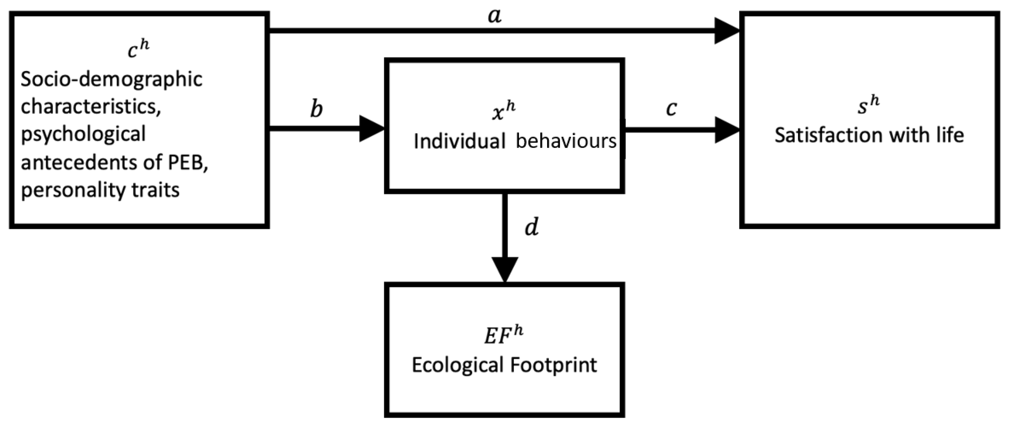
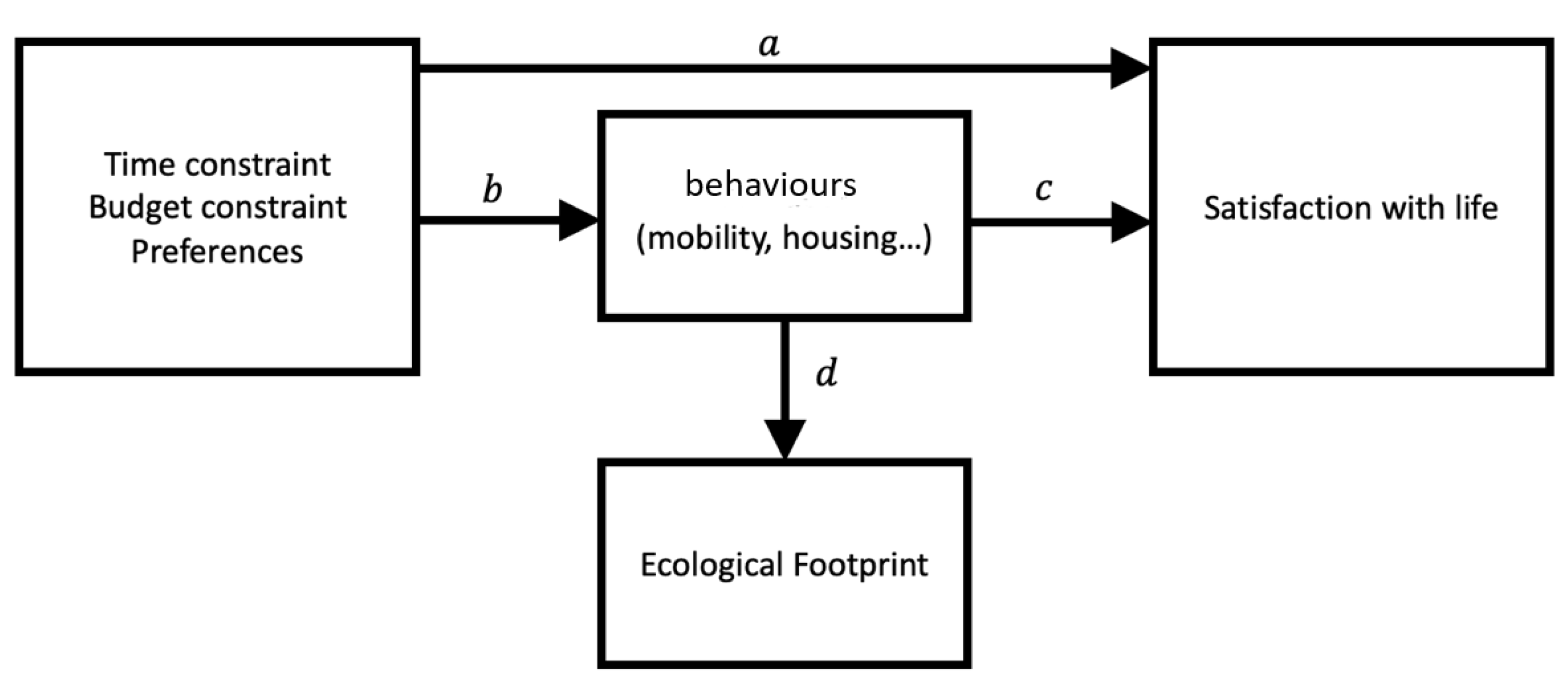
Figure 1 summarises. An individual is confronted with time constraints and budget constraints and has preferences that are represented in decision utility. Arrow b represents the process in which the individual decides on a number of pro-environmental behaviours (mobility, housing, etc.). Arrow d shows how these behaviours result in the ecological footprint, a measure of the aggregated environmental impact of the individual. The choice of behaviours also causes the individual’s experienced utility: satisfaction with life, represented by arrow c. Of course, satisfaction with life can be also influenced by many other factors, which is shown in arrow a. Below, we look at two aspects. First (arrow b) we analyse the determinants of the individual behaviours in seven different components of the ecological footprint: food, energy use (housing and electricity), paper use, and mobility (car use, public transport, travelling). Second (arrow c), we analyse the way these behaviours are associated with satisfaction with life. We use socio-demographic characteristics (income, family size, age, etc.) and a number of psychological antecedents of pro-environmental behaviour as signalling information on the constraints and the preferences. The satisfaction with life model (arrows a and c in Figure 1) is estimated as a mediation model in which the individual socio-demographic characteristics and the psychological antecedents of pro-environmental behaviour are associated with satisfaction with life both directly and indirectly [17,19,24].

A better understanding of the extent to which the behavioural change impacts each of the components of the ecological footprint and the ecological footprint as a whole at the individual level, and satisfaction with life at the individual level, is important in order to design policy interventions. The analysis in this article does exactly that: it does not focus on one type of behaviour (e.g., recycling, energy use or mobility) but looks at the ecological footprint at the individual level (like [10,19,23]).

We use the LEVO 2017 survey, which has been conducted in Flanders (Belgium). This survey contains, for 1763 respondents, information on their socio-demographic characteristics, psychological antecedents of pro-environmental behaviour, behaviours related to the seven components of the ecological footprint, and satisfaction with life. This data set will be used to reach the two main objectives of this article.

The next section introduces the theoretical model, Section 3 deals with the empirical application, and Section 4 concludes.

2. Theoretical Model

This section presents the micro-economic model behind our analysis. First, the basic model is presented, in which all choices are continuous variables; then, we proceed by looking at the consequences of the fact that many choices are of a discrete nature. In the exposition, we also allow for preference differences across individuals in terms of decision utility.

2.1. Basic Model

There are H individuals in the economy. The individual’s life situation consists of a bundle of I behaviours $x^h=\left(x_1^h,\cdots ,x_I^h\right)$. At the moment of decision making, decision utility $u^h\left(x^h\right)$ is used. The individual derives experienced utility $s^h\left(x^h\right)$, which is satisfaction with life. The $x^h$ are behaviours in terms of seven EF components: food consumption, housing, energy use, private mobility (car use), public transport, paper use, and travelling. For each of the components, there are several options. In the footprint calculator of Ecolife vzw that we use, for example, for food, there is the choice between locally produced food, fresh products, frozen vegetables, whether or not to eat meat, and so on. For mobility, there is car, bike, or public transport. In general, for behaviour i, individual h has J options $x_{i1}^h,\dots ,x_{ij}^h,\dots ,x_{iJ}^h$. The list of behaviours and the list of options for each behaviour used in this article is provided in Appendix A.

The individual’s choice set is limited in two ways: by a budget constraint $M^h$ and by a time constraint $T^h$. Each of individual h’s options $x_{ij}^h$ has a price $p_{ij}^h$ and a time cost $t_{ij}^h$. Consequently, individual h is confronted with the constraint ${\sum }_{i=1}^I{\sum }_{j=1}^J{t}_{ij}^h{x}_{ij}^h\le T^h$ ($TC$, time constraint) and ${\sum }_{i=1}^I{\sum }_{j=1}^J{p}_{ij}^h{x}_{ij}^h\le M^h$ ($BC$, budget constraint). Both the prices and the time costs are specific to the individual. For example, someone in the city might have easier access to organic food, so it takes less time to acquire it. The same applies to mobility: someone living in the city has better access to public transport, which results in a lower time cost for the use of public transport. Other aspects of life also influence these constraints, for instance, someone who has to bring children to school might face different time constraints in terms of mobility. Prices individuals face for the behaviours differ as well (e.g., someone in the city faces higher rental prices than someone on the countryside).

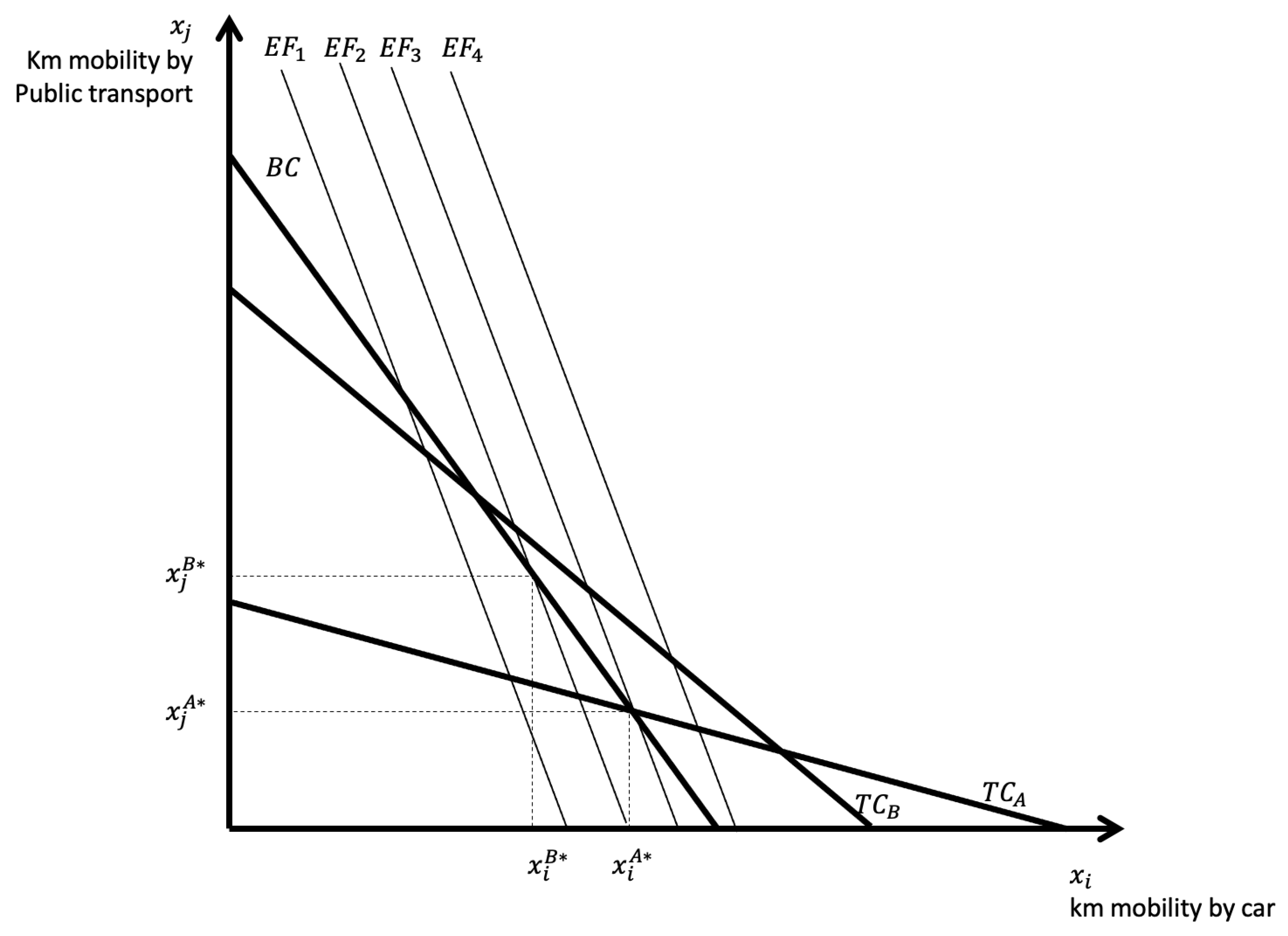
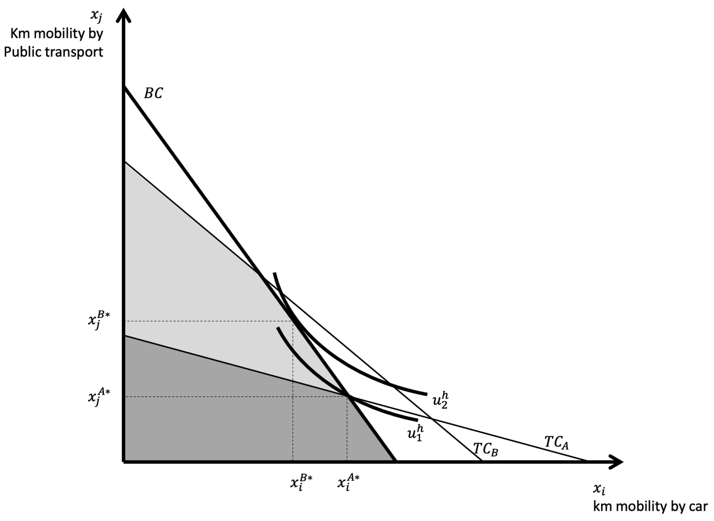
Figure 2 illustrates the case of mobility. On the horizontal and the vertical axes, the number of kilometers travelled by car and by public transport are shown. The line $BC$ represents the budget constraint for two individuals A and B, assuming that they are facing the same prices. The time constraint for the two individuals differs, though. Individual A might live on the countryside with less access to public transport and with less traffic. With the same amount of time, a larger distance by car and a lower distance by public transport can be realised. Individual A’s available options are represented by the dark grey shaded area; this is the common surface below both $BC$ and $T{C}_A$. Individual B lives in the city, where access to public transport is easier, so travelling by bus or tram is less time consuming, but traffic renders car use more time intensive. This is represented by $T{C}_B$. Individual B’s options are represented by both shaded areas.

We assume that individuals maximise the decision utility $u^h\left(x^h\right)$ subject to the two constraints. This results in an individual choice of behaviours depending on the time and income constraints: $x^{h*}=x^h\left(p^h,t^h,M^h,T^h\right)$. In Figure 2, two indifference curves are shown, under the assumption that individual A and individual B have the same preferences (i.e., the same utility function). The individuals make different decisions: individual A uses the car more often and public transport less often than individual B.

Each of the behaviours also has an influence on the individual’s EF: each option $x_{ij}$ has a footprint of $e_{ij}$. An individual’s choices consequently lead to the individual’s ecological footprint: ${\mathrm{EF}}^h=\mathrm{EF}\left(x^{h*}\right)$. In Figure 3, four different levels of the EF are represented, where the iso-EF curve ${\mathrm{EF}}_1$ represents the lowest level and iso-EF curve ${\mathrm{EF}}_4$ is the highest level. An increase in total mobility leads to a higher EF, and mobility by car has a bigger impact on the EF than mobility by public transport, which renders the iso-EF lines rather steep. In the figure, household A’s choices lead to a higher level of EF than individual B’s choices.

Each individual h has C characteristics $c^h=\left(c_1^h,\dots ,c_C^h\right)$. This list of characteristics also contains, apart from socio-demographic characteristics such as family size, income, and educational attainment, psychological antecedents of pro-environmental behaviour and personality traits.

These characteristics both influence the budget and time constraints, and the individual’s preferences, represented in their decision utility function. The influence on the constraints is shown in Figure 2. Figure 4 shows the impact of different preferences, which means that the decision utility differs across individuals. In this figure, both individuals have a preference for public transport compared to car use, so the indifference curves are less steep than in Figure 2. This results in different choices: both individuals use the car less often and make more use of public transport than in Figure 2.

Consequently, we assume that information on the budget and time constraints is incorporated in the individual characteristics, and the individual behavioural choices depend on the individual characteristics $c^h$: $x^h\left(p^h,t^h,M^h,T^h\right)=x^h\left(c^h\right)$. This is the case both because the characteristics influence the two constraints and because they might influence the individual’s preferences. Consequently, the individual characteristics can both constrain and facilitate pro-environmental behaviour.

2.2. Discrete Choice

In the previous exposition, the behavioural choices were presented as continuous variables (number of kilometers in Figure 2, Figure 3 and Figure 4). Many of the individual behaviours are to a large extent discrete choices, though, as is also the case in the questions concerning the ecological footprint (see Appendix A). Take the example of heating fuel for the house, which can be gas, heating oil, wood, electricity, and so on. We pay explicit attention to this type of choice, as it can influence the individuals’ constraints as well as their decision utility function. We take the example of meat and fish consumption and of car use. For the consumption of meat and fish, the individuals have the choice between ‘never’, ‘sometimes 1–3 times per week’, ‘4–5 times per week’, ‘daily around 200 g’, and ‘daily more than 200 g’. The first option entails the lowest EF, and the last option entails the highest EF. First of all, from the perspective of the budget constraint, it is not clear which option is the cheapest and which option is the most expensive. The monetary and time costs of each of these options depends on the individual characteristics. In cities, for instance, vegetarian alternatives might be easier to find than in the countryside. Similarly, individuals with different characteristics might face different time constraints. Finding vegetarian or organic food might take more time than going to the regular supermarket. For car use there is the choice between ‘never/ we have no car’, ‘seldom’, ‘daily for less than 50 km’, ‘daily between 50 km and 100 km’, and ‘daily average of more than 100 km’. Here, as well, both the budget constraint and the time constraint depend on the individual characteristics. An individual living far away from work might have to drive far to get to work. This is expensive if the individual has no access to a company-provided car. On the other hand, those seeking alternatives to owning a car might nevertheless spend a lot on mobility (e.g., by buying an electric bike, subscriptions for car sharing, etc.).

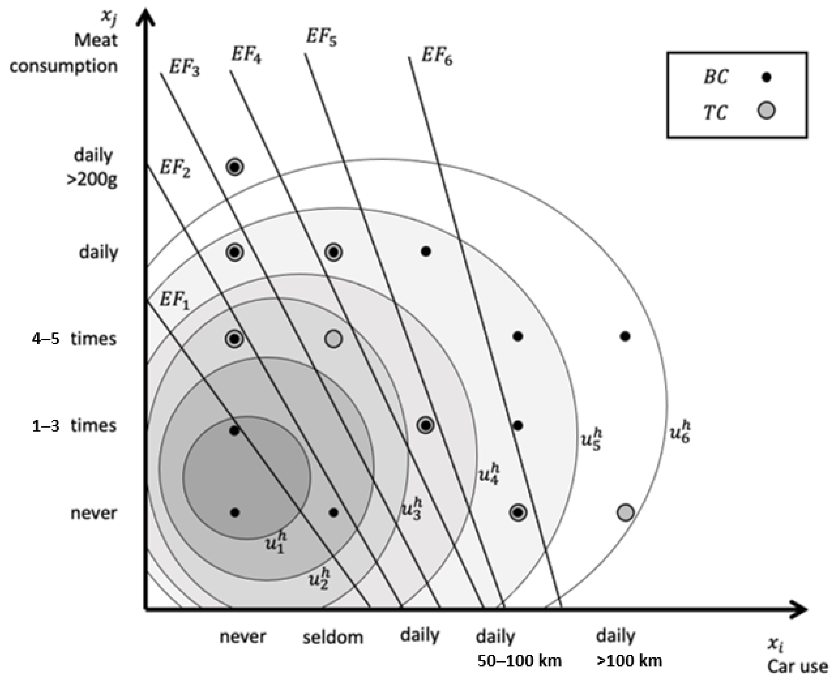
In the example in Figure 5, a (hypothetical) feasible combination of car use and meat choice according to the budget constraint (BC) is marked with a black circle and a feasible combination in terms of the time constraint (TC) is marked with a grey circle. For instance, in the figure, the combination of ‘seldom eating meat’ and ‘driving the car 4–5 times per week’ satisfies the time constraint but not the budget constraint. The combination of never eating meat and never using the car satisfies the budget constraint but not the time constraint. Note that the individual in the example has six available options satisfying both the BC and the TC. The iso-EF lines represent levels of the ecological footprint resulting from the different combinations, with ${\mathrm{EF}}_6$ the highest level and ${\mathrm{EF}}_1$ the lowest level. The option with the lowest EF available to the individual is to never use the car and to eat meat 4–5 times a week. The available option with the highest EF is to use the car daily for 50–100 km and to never eat meat (bottom right in Figure 5).

The individual’s choice depends on their judgment of each of the options represented in the utility function. There is no clear hierarchy in the options presented in Figure 5, so utility is not per se strictly increasing in the behaviours. For someone who likes driving the car and eating meat, for example, utility will be increasing both in car use and in meat consumption. However, for a vegetarian, for instance, things might be different, which will be represented in the shape of the indifference curves. In any case, the judgment about what is the most attractive choice can differ between individuals. Figure 5 provides a fictive example of indifference curves (indifference contours) for an individual with preferences for low meat consumption and for limiting car use, with $u_1^h$ the highest utility level and $u_6^h$ the lowest one. The individual’s most preferred situation $u_1^h$ is where they never use the car and eat meat either never or 1–3 times a week. These two options at the bottom left of Figure 5 are unavailable to the individual, as they don’t satisfy the time constraint. One reason could be that there are no shops selling alternatives to meat close to the individual’s house (e.g., organic shops). Without a car, fetching these alternatives takes a lot of time. Consequently, this individual might choose to not use a car and to eat meat 4–5 times per week, which yields a higher (decision) utility than the other feasible choices.

2.3. Model Structure

This section provides information on the model we will use for the empirical analysis. Figure 6 provides an overview of the empirical model, based on Figure 1. As we do not use individual specific information on prices and time use for each of the behaviours, we focus on individual characteristics as determinants. This means that the individual characteristics influence both the constraints and the individual preferences. We aim to study two aspects. First, we study the influence of individual characteristics $c^h$ on a number of individual behaviours $c^h$ related to the ecological footprint. In Figure 6, this means that arrows b and d are studied. Arrow b represents the impact of a change in $c^h$ on $x^h$, while arrow d represents the impact of a change in $x^h$ on the ecological footprint.

The second aim of the article is to study the impact on welfare, which we equate here to satisfaction with life $s^h$. In Figure 6, this is represented by arrows a, b, and c, in a mediation model. Arrow a represents the direct effect of the individual characteristics on satisfaction with life, while arrows b and c represent the effect of characteristics via individual behaviours. Below, we will provide empirical estimates of the size of the effects of arrows a, b, and c. Arrow d is based on technical information on the calculated ecological footprint.

3. Results and Discussion

This section deals with the results and the discussion, based on the empirical analysis. Our aim is to analyse the determinants of the behaviours underlying the ecological footprint, and their association with satisfaction with life (well-being). The first paragraph below deals with the influence of the individual behaviours on the ecological footprint (arrow d). Here, we need only information on the technical calculation of the ecological footprint. The second paragraph deals with the arrows a, b, and c in the figure, which will be based on statistical analysis, using an empirical estimation based on the LEVO 2017 data, collected in Belgium. This will inform us about the socio-demographic determinants and psychological antecedents of the choices households make. This will result in an analysis of the impact of the individual characteristics on both the EF (arrows b and d) and on satisfaction with life (arrows a, b, and c).

3.1. Individual Behaviours and the Ecological Footprint: A Technical/Methodological Relation

In this section, we pay attention to the impact of individual behaviours on the EF (arrow d) in Figure 6. This can be retrieved from the technical calculation of the ecological footprint. Here, we use an EF calculator that has been calibrated for Belgium by Ecolife vzw, a Belgian knowledge centre for footprinting and ecological behavioural change. The methodology is based on the WWF methodology and calibrated based on the 2010 Global Footprint Network National Footprint Accounts. It provides us with information on the slopes of the iso-EF lines in Figure 2, Figure 4, and Figure 5. The individual ecological footprint is based on seven EF components. Information on these seven components depends on the ten questions in Appendix A. The seven components are food (questions 1 and 2), housing (questions 3, 4, and 5), electricity use (question 6), paper use (question 7), car use (question 8), public transport (question 9), and travel (question 10). For some of these components, family size plays a role (e.g., because a house or a car can be shared among family members).

We start with the EF of car use (see question 8 from Appendix A, the options of which are provided in

Table 1. Individual behaviour and EF for car use $x_8$.

	Family Size	1	2	3	5
car use	never	0	0	0	0
$x_8$	seldom	0.244	0.244	0.244	0.244
	daily < 50 km	1.466	0.855	0.651	0.489
	daily 50–100 km	3.908	2.076	1.466	0.977
	daily > 100 km	6.350	3.297	2.280	1.466

Each number in the table is the ecological footprint of a choice of car use, for families of different sizes. Source: Ecolife vzw.

). Each of the entries in the table provides the number of global hectares associated with a specific choice in terms of car use. As cars are shared among household members, family size plays a role. From this table, for instance, if a household of three members changes its behaviour from using the car daily to seldom, the EF from car use reduces from 0.651 gha to 0.244 gha, which is a reduction of 0.407 gha.

Information on the food footprint is provided in

Table 2. Individual behaviour and the EF for food.

		Food Choice in Terms of Vegetables ${\mathit{x}}_{\mathbf{1}}$
	Answer	Local	Mainly	Frozen	Restaurant
		Seasonal	Fresh	Preserves
meat	never	1.109	1.204	1.347	1.538
$x_2$	1–3 per week	1.321	1.429	1.587	1.791
	4–5 per week	2.070	2.365	2.424	2.674
	daily	2.295	2.451	2.675	2.938
	daily > 200 g	2.821	3.009	3.275	3.576

Note: Entries in the table are the ecological footprint expressed in gha for a choice related to food, in terms of the quantity of meat consumed (vertical) and in terms of vegetable consumption (horizontal). Source: Ecolife vzw.

, based on questions 1 and 2 from Appendix A. The choice options for each of these questions is provided in the table. Each table entry provides the EF for the food component (expressed in global hectares) based on individual choices related to food. Imagine an individual who chooses ‘mainly fresh products’ for the first question $x_1$ and says they eat meat ‘4–5 times a week’ for the second question $x_2$. This person has a footprint of 2.365 for the food component. If meat consumption is reduced to 1–3 times a week, then the EF diminishes to 1.429. Note that the maximum gain to be made is a move from an EF score for food of 3.576 (bottom right corner of the table) to an EF score of 1.109 (top left corner of the table), a decrease of 2.467 gha, but this obviously requires a huge behavioural change.

The EF of electricity, paper, public transport, and travel are provided in Appendix A. The EF of housing is based on a combination of behaviours from questions 3, 4, and 5 in Appendix A.

One remark is in order concerning family size, one of the characteristics in $c^h$. Family size influences household choice (a larger family needs a bigger house), and family size influences the relationship between the behaviour and the ecological footprint (heating is shared among family members, so adding extra members actually reduces the EF per member). This applies only to the aspects that are shared among the family members, such as housing. It does not apply to food, for instance, which is consumed individually.

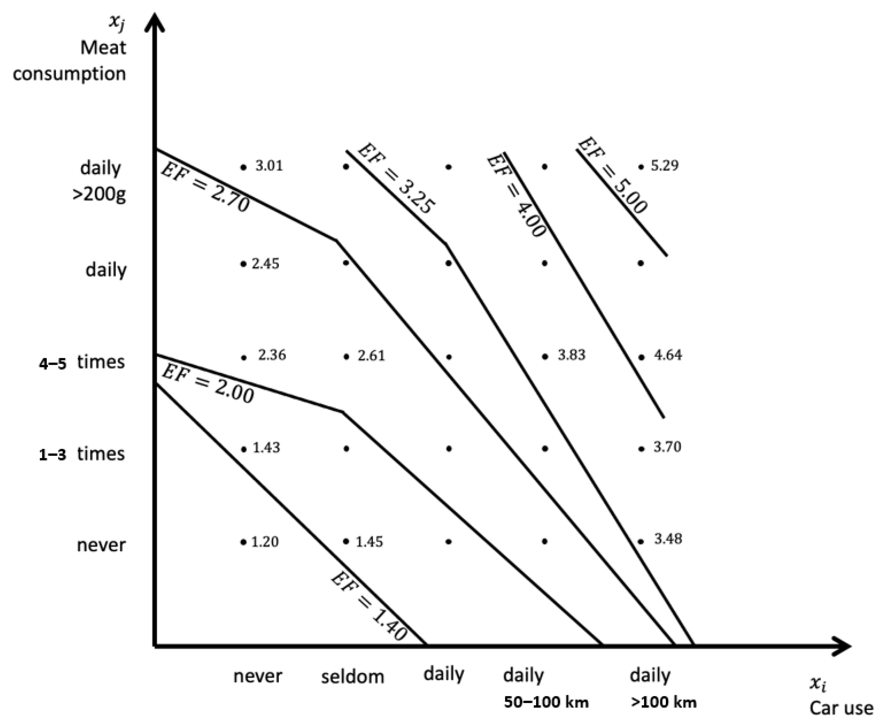
Figure 7 represents the EF for all choice options in terms of car use and meat consumption. The situation is represented for an individual in a household with three members (see Table 1) and who consumes mainly fresh food (see Table 2). Each dot in the figure represents a choice combination, and the lines represent iso-EF curves for different levels. Numbers next to the dots refer to the ecological footprint of the combination of these choices, expressed in gha.

3.2. Individual Characteristics, Behaviours, and Satisfaction with Life: A Statistical Relation

This section deals with arrows a, b, and c in Figure 6. We analyse empirically how the individual characteristics are associated with the individual behaviours, and how the behaviours, in turn, lead to satisfaction with life. The next two paragraphs provide information on the data set and on the estimation results.

3.2.1. The LEVO Data Set

We use the LEVO 2017 data set that has been collected in Flanders, Belgium. It is a cross-sectional data set that contains survey questions about living conditions, questions about socio-demographic determinants and personality traits, questions about values and judgments about environmental behaviour (the psychological antecedents), questions on behaviours related to the EF, and questions related to satisfaction with life. The surveys have been conducted in person by trained enumerators, and fully follow the ethical code of the Faculty of Economics and Business Administration of Ghent University. For each family, one adult member has been interviewed. The individual information relates to this person, and all information concerning family-related variables (family size, housing) has been answered by this person. The data set contains extensive cross-sectional information. In total there are 2035 respondents, of which 1763 remain after the elimination of students and those with information missing and other data cleaning. The data set allows us to calculate the ecological footprint at the individual level, which is uncommon in the literature (exceptions are [10,19,23]). Most data sets contain information on the ecological footprint at the aggregated level (country, region, or group of people). The ecological footprint is calculated based on ten questions inquiring into the individual behaviours (see Appendix A for the list of questions). The relatively small number of EF questions has to do with the fact that the LEVO survey is already of considerable length.

Table 3. Summary statistics of LEVO data, $N=1763$.

Name	Min	Max	Mean	St.dev
$c_1$ Abstract knowledge	1	7	4.39	1.31
$c_2$ Concrete knowledge	1	7	4.15	0.95
$c_3$ Environmental self-identity	1	7	4.15	1.17
$c_4$ Parents speak	1	7	2.68	1.46
$c_5$ Parents act	1	7	2.78	1.46
$c_6$ Environmental concern	1	7	4.57	1.35
$c_7$ Dummy male	0	1	0.496
$c_8$ Equivalised income (in 000 EUR)	0	7.25	1.972	0.951
$c_9$ Family size	1	9	3.176	1.326
$c_{10}$ Dummy neighbourhood centre (village or town) (5)	0	1	0.333
$c_{11}$ Dummy neighbourhood city centre (5)	0	1	0.135
$c_{12}$ Dummy neighbourhood countryside (5)	0	1	0.298
$c_{13}$ Dummy neighbourhood suburban (5)	0	1	0.234
$c_{14}$ Age	18	91	47.640	17.746
$c_{15}$ Dummy primary education	0	1	0.064
$c_{16}$ Dummy lower secondary education	0	1	0.152
$c_{17}$ Dummy higher secondary education	0	1	0.389
$c_{18}$ Dummy bachelor	0	1	0.240
$c_{19}$ Dummy >master	0	1	0.156
$c_{20}$ Political point of view economic (left wing/right wing)	0	9	5.600	1.993
$c_{21}$ Political point of view ethical (left wing/right wing)	0	9	4.730	1.902
$c_{22}$ Extraversion	−3.0	3.0	−1.037	1.668
$c_{23}$ Agreeableness	−3.0	3.0	0.392	1.683
$c_{24}$ Neuroticism	−3.0	3.0	−0.440	1.612
$c_{25}$ Conscientiousness	−3.0	3.0	1.010	1.500
$c_{26}$ Openness to experience	−3.0	3.0	−0.126	1.547
$c_{27}$ Integrity	−3.0	3.0	1.789	1.247
Ecological footprint, food component	1.11	3.58	2.212	0.459
Ecological footprint, housing component	0.24	8.75	2.225	1.289
Ecological footprint, electricity use component	0	2.58	0.521	0.378
Ecological footprint, paper use component	0.01	1.17	0.339	0.211
Ecological footprint, car use component	0	6.35	0.817	0.633
Ecological footprint, public transport component	0	0.99	0.115	0.117
Ecological footprint, travel component	0	1.57	0.541	0.498
$\mathrm{EF}$ Ecological footprint (total)	2.408	19.065	6.770	1.854
Satisfaction with life in general	1	10	7.726	1.160

Note: the data are based on the LEVO 2017 questionnaire.

provides summary statistics of the individual characteristics, marked with $c_i$, and the ecological footprint split up per footprint component.

First, we deal with the six psychological antecedents of environmental behaviour we use in this study, available from the LEVO2017 data set. These are abstract knowledge ($c_1$) and concrete knowledge ($c_2$), environmental self-identity ($c_3$), the extent to which parents speak about the environment ($c_4$), parental behaviour related to the environment ($c_5$), and environmental concern ($c_6$). Abstract knowledge is measured by the question ‘Environmental problems encompass inter alia air pollution, water pollution, waste and waste disposal, climate change and natural resource depletion, how much do you know about environmental problems’, on a seven-point Likert scale ranging from ‘very little’ to ‘a lot’. In the literature [33,40], different multi-item measurement scales are proposed, but unfortunately, the LEVO2017 data set only contains this question on abstract knowledge. Concrete knowledge is measured with several items, in line with Frick et al. (2004) [40], as the average of three statements: ‘I actively search info to decrease my impact on the environment’, ‘I know how to change behaviour to decrease my environmental impact’, and ‘I know which concrete actions to decrease my environmental impact’, each of which is answered on a seven-point Likert scale (Cronbach’s alpha is equal to 0.644). Both abstract and concrete knowledge are self-reported. It is the individual’s own judgment about her or his knowledge, which is not per se correct. Unfortunately, with the LEVO data set, we cannot do better than keeping this issue in mind when interpreting the results. Environmental self-identity is calculated as the average of three statements: ‘Behaving in an environmentally friendly way is an important part of who I am’, ‘I am the type of person that behaves in an environmentally friendly way’, and ‘I see myself as an environmentally friendly person’ (all on a seven-point Likert scale ranging from ‘strongly disagree’ to ‘strongly agree’). The Cronbach’s alpha for our indicator of environmental self-identity is equal to 0.878. Parental behaviour is split up into what parents say about behaving in an environmentally friendly way and how parents actually behave. The former is based on the statement ‘during my youth my parents took environmental issues into consideration in their decisions’, while the latter is based on the statement ‘during my youth my parents spoke about the environment’. Both are based on a seven-point Likert scale with answers ranging from ‘completely disagree’ to ‘completely agree’. These two questions are based on Eagles and Demare (1999) [42], except that they use a five-point Likert scale. Finally, environmental concern is based on the question ‘How concerned are you about environmental issues?’, measured on a scale ranging from ‘not concerned at all’ to ‘very concerned’. Again, in the literature, multi-item measurement scales are proposed (e.g., the Ecological Attitude Scale or the New Environmental Paradigm scale in Fransson and Gärling (1999) [28]), but the LEVO2017 questionnaire provides us only with one question. Even if the LEVO 2017 questionnaire contains extensive information on socio-demographic variables and allows us to calculate the ecological footprint at the individual level, a shortcoming of the LEVO 2017 questionnaire is that it does not contain information on other psychological antecedents from the literature such as moral norms, biospheric value orientation, or behavioural control. To some extent, the information on parental behaviour could provide some information on environmental norms.

The next two blocks contain the socio-demographic characteristics and the character traits. The first block provides socio-demographic information such as age, income, and education. Equivalised income is calculated as family income divided by the square root of family size. There are two questions on the respondent’s political-economic and political-ethical stance. In terms of political point of view, a distinction is made between economic ‘left wing/right wing’ (socialist to liberal) and ethical ‘left wing/right wing’ (progressive to conservative). Each of the questions is based on a scale of ten points, from 0 to 9. The second block contains information on the respondent’s personality: the big five personality traits combined with integrity [44,45].

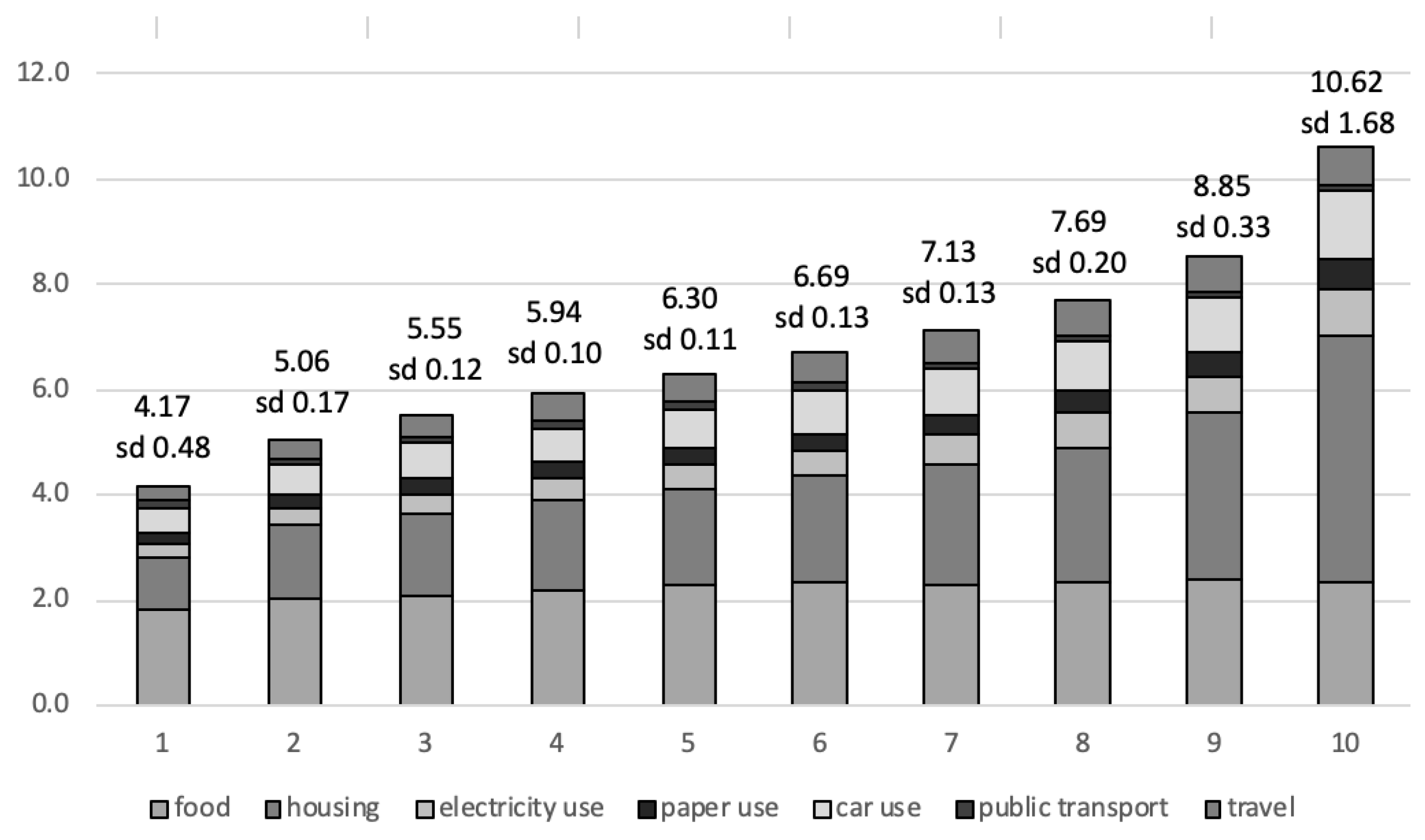
The third block of Table 3 contains information on the components of the ecological footprint, based on the behaviours $x^h$, for which the questions are available in Appendix A. A table entry provides the EF score of a component, expressed in global hectares (gha). For example, the average ecological footprint for the food component amounts to 2.212 in our sample. The average total EF is 6.770 global hectares, which is the sum of the seven EF scores for each of the components. Note that most of the total EF depends on choices related to food and housing (2.212 + 2.225 = 4.437 gha). Figure 8 and Figure 9 contain information on the distribution of the ecological footprint across observations in the sample. Finally, the last line of Table 3 contains the question on satisfaction with life. The survey contains a standard satisfaction with life question: “Taken everything into consideration, I am satisfied with my life” (see [46] for a discussion). Respondents have to give themselves a score between 1 (marked with ‘very unsatisfied’) and 10 (marked with ‘very satisfied’). Table 3 shows that the average score in the LEVO2917 sample is 7.726.

3.2.2. Estimation

In this section, the household decision-making process is empirically analysed, as the combination of arrows a, b, and c from Figure 6. First, in

Table 4. Multinomial regression results: determinants of behaviours related to food and fuel use (arrow b).

Type	${\mathit{x}}_1$ Food			${\mathit{x}}_5$ Fuel
Choice	Seasonal	Frozen	Prepared	Gas	Wood	Elec	Green
	Local	Abroad	Restaurant				Elec
$c_1$ Abstract knowledge
$c_2$ Concrete knowledge							0.398 *
$c_3$ Env. Self-id.		−0.625 ***	−0.380 **	−0.251 ***	0.417 *	−0.354 ***
$c_4$ Parents speak
$c_5$ Parents act		0.273 ***				0.179 **
$c_6$ Env. concern			−0.338 **	0.233 ***
$c_7$ Dummy male		0.545 ***
$c_8$ Eq. income in 000EUR					−0.408 **		0.445 ***
$c_9$ Dummy Famsize 2		−1.143 ***	−1.192 ***			−0.599 *
$c_9$ Dummy Famsize 3		−0.849 *	−1.813 ***
$c_9$ Dummy Famsize 4		−0.882 **	−1.984 ***			−0.939 ***
$c_9$ Dummy Famsize > 4		−0.783 *	−1.833 ***			−0.775 **
$c_{10}$ Dummy village centre	−0.328 **	0.816 **	1.056 *	−1.039 ***	−1.510 ***	0.817 ***	0.600 *
$c_{11}$ Dummy city centre		0.992 **	1.991 ***	1.577 ***		1.385 ***
$c_{13}$ Dummy suburban	−0.360 **	0.839 **	1.119 *	−1.255 ***	−1.012 **	0.843 *	1.007 ***
$c_{14}$ Age	0.012 ***		−0.020 *	−0.012 **	−0.027 **	−0.021 ***	−0.026 **
$c_{15}$ Dummy prim educ		−1.606 ***
$c_{17}$ Dummy lower sec educ					0.973 **
$c_{18}$ Dummy bachelor			−0.830 *
$c_{19}$ Dummy Master	−0.409 **
$c_{20}$ Poleconomic	0.050 *
$c_{21}$ Polethical
$c_{22}$ Extroversion		0.126 *
$c_{23}$ Agreeableness			0.160 *		−0.220 ***		0.194 **
$c_{24}$ Neuroticism		0.147 *		−0.087 **
$c_{25}$ Conscientiousness		−0.190 ***
$c_{26}$ Openness to experience	−0.091 **
$c_{27}$ Integrity	0.206 ***	−0.257 ***				1.101 *
Intercept	−2.258 **						−3.038 ***
Nagelkerke $R^2$	0.223			0.196

Notes: *, **, and *** refer to significance at the 10%, 5%, and 1% level, respectively. The reference category for food is ‘mainly fresh products’; the reference category for fuel is ‘heating oil’. The reference category for family size is ‘one member’; for place of residence, it is ‘countryside rural’; and for education, it is ‘high school education’.

,

Table 5. Ordinal regression results: determinants of behaviours for meat consumption, housing, heating, and electricity (arrow b).

Type	${\mathit{x}}_2$	${\mathit{x}}_3$	${\mathit{x}}_4$	${\mathit{x}}_6$
	Meat	House Size	Heat	Elec
$c_1$ Abstract knowledge	0.104 **
$c_2$ Concrete knowledge	−0.105 *			−0.270 ***
$c_3$ Env. self-id.	−0.104 *			−0.460 ***
$c_4$ Parents speak	−0.083 **
$c_5$ Parents act			−0.100 **
$c_6$ Env. concern	−0.186 ***
$c_7$ Dummy male	0.552 ***
$c_8$ Eq. income in 000 EUR		0.296 ***	−0.104 *
$c_9$ Dummy famsize 2	0.388 **	0.680 ***	−0.317 *
$c_9$ Dummy famsize 3	0.500 ***	1.284 ***	−0.360 *
$c_9$ Dummy famsize 4	0.411 **	1.804 ***	−0.508 ***
$c_9$ Dummy famsize > 4	0.481 **	2.418 ***	−0.394 *
$c_{10}$ Dummy village centre	−0.210 *	−1.151 ***	−0.289 **
$c_{11}$ Dummy city centre	−0.517 ***	−1.738 ***
$c_{13}$ Dummy suburban		−0.816 ***
$c_{14}$ Age		0.019 ***	0.012 ***
$c_{15}$ Dummy prim educ
$c_{17}$ Dummy lower sec educ		−0.319 **
$c_{18}$ Dummy bachelor		0.195 *
$c_{19}$ Dummy master	−0.535 ***	0.448 ***		0.311 **
$c_{20}$ Poleconomic		0.108 ***		0.055 **
$c_{21}$ Polethical		−0.050 *		−0.048*
$c_{22}$ Extroversion
$c_{23}$ Agreeableness
$c_{24}$ Neuroticism			0.070 **
$c_{25}$ Conscientiousness		0.063 **	−0.078 **
$c_{26}$ Openness to experience
$c_{27}$ Integrity	0.066 *
Threshold 1	−5.383 ***	−3.008 ***	−3.305 ***	−5.949 **
Threshold 2	−2.081 ***	−0.789 **	−0.452	−3.133 ***
Threshold 3	−0.215	0.686 *	0.624 *	0.394
Threshold 4	2.008 ***	2.559 ***
Threshold 5		3.025 ***
Nagelkerke $R^2$	0.098	0.298	0.074	0.174

Notes: *, **, and *** refer to significance at the 10%, 5%, and 1% level, respectively. The reference category for family size is ‘one’; for place of residence, it is ‘countryside rural’; and for education, it is ‘high school education’.

and

Table 6. Ordinal regression results: determinants of choices in terms of paper use, car use, public transport, and travel (arrow b).

Type	${\mathit{x}}_7$	${\mathit{x}}_8$	${\mathit{x}}_9$	${\mathit{x}}_{10}$
	Paper	Car	Pubtr	Travel
$c_1$ Abstract knowledge
$c_2$ Concrete knowledge	−0.134 **		0.145 **
$c_3$ Env. self-id.	−0.258 ***	−0.188 ***		−0.117 **
$c_4$ Parents speak
$c_5$ Parents act	−0.076 *	−0.077 *
$c_6$ Env. concern	−0.104 **		0.095 **
$c_7$ Dummy male	0.328 ***			0.193 *
$c_8$ Eq. income in 000 EUR		0.399 ***		0.109 **
$c_9$ Dummy famsize 2		0.806 ***
$c_9$ Dummy famsize 3		1.594 ***	0.645 **	0.422 **
$c_9$ Dummy famsize 4		1.965 ***	0.791 ***	0.496 ***
$c_9$ Dummy famsize more than 4		1.900 ***	1.210 ***
$c_{10}$ Dummy village centre		−0.427 ***
$c_{11}$ Dummy city centre		−0.813 ***	0.368 **
$c_{13}$ Dummy suburban		−0.430 ***
$c_{14}$ Age		−0.026 ***	−0.006 *
$c_{15}$ Dummy prim educ		−0.393 *	−0.506 **
$c_{17}$ Dummy lower sec educ
$c_{18}$ Dummy bachelor		0.301 ***		−0.217*
$c_{19}$ Dummy master		0.530 ***
$c_{20}$ Poleconomic		0.071 ***	−0.079 ***
$c_{21}$ Polethical
$c_{22}$ Extroversion
$c_{23}$ Agreeableness
$c_{24}$ Neuroticism		0.113 ***
$c_{25}$ Conscientiousness	0.060 *	−0.087 **	−0.069 **
$c_{26}$ Openness to experience		−0.068 **
$c_{27}$ Integrity
Threshold 1	−5.106 ***	−3.211 ***	−0.371	−0.242
Threshold 2	−2.915 ***	−1.207 ***	2.403 ***	0.001
Threshold 3	0.164	2.012 ***	4.311 ***	0.106
Threshold 4		3.804 ***	6.030 ***	0.919 **
Threshold 5				2.597 ***
Nagelkerke $R^2$	0.113	0.322	0.122	0.028

Notes: *, **, and *** refer to significance at 10%, 5%, and 1% level, respectively. The reference category for family size is ‘one’; for place of residence, it is ‘countryside rural’; and for education, it is ‘high school education’.

we focus on the determinants of the individual behaviours: how they are associated with individual characteristics (arrow b from Figure 6). Then, in

Table 7. Estimation results for satisfaction with life $s^h$: arrows a and c.

Dependent Variable	${\mathit{s}}^{\mathit{h}}$ Direct + Indirect	${\mathit{s}}^{\mathit{h}}$ Total
$c_6$ Environmental concern	0.051 **	0.052 **
$c_8$ Eq. income in 000 EUR	0.111 ***	0.150 ***
$c_9$ Dummy famsize = 2	0.215 **	0.360 ***
$c_9$ Dummy famsize = 4		0.256 **
$c_9$ Dummy famsize > 4		0.292 **
$c_{20}$ Potical economic	0.048 ***	0.057 ****
$c_{22}$ Extroversion	−0.095 ***	−0.098 ***
$c_{23}$ Agreeableness	0.053 ***	0.054 ***
$c_{24}$ Neuroricism	−0.105 ***	−0.113 ***
$c_{25}$ Conscientiousness	0.040 **	0.054 **
$c_{27}$ Integrity	0.095 ***	0.108 ***
$x_3$ Average (semi-) detached house	0.294 ***
$x_3$ Large apartment of terraced house	0.330 ***
$x_3$ Large (semi-) detached house	0.354 ***
$x_{10}$ Travel in Europe by train/bus	0.360 **
Intercept	6.081 ***
Adjusted $R^2$	0.170	0.165

Notes: ** and *** refer to significance at the 5% and 1% level, respectively. In the first estimation, all behaviours and all characteristics have been incorporated, but only those coefficient significantly different from zero are provided, in order to save space. In the second estimation, only the individual characteristics are taken into consideration.

, we focus on the way the characteristics and the behaviours are associated with satisfaction with life (arrows a an c). In the case of food $x_1$ and heating $x_5$, there is no ordering in the answers, so the model will be estimated as a multinomial logit (see Table 4). The other eight behaviours will be estimated as an ordered logit model (see Table 5 and Table 6). The dependent variables are the individual characteristics. In order to take account of the number of members of each family, the family size variable is transformed into dummies (for each family size). That will allow us to distinguish between types of families.

In Table 4, we focus on the decision-making process related to behaviour 1 for food (with the reference category ‘mainly fresh products’) and behaviour 5 for fuel for heating (the reference category is ‘gas’). The numbers provided in the table are interpreted as probabilities relative to the reference category. Only those betas are provided in the table that are significantly different from zero. The coefficient is to be interpreted as the extra probability of choosing a specific behaviour, compared to the reference category, if one of the determinants of pro-environmental behaviour changes one unit. A positive (negative) coefficient means that a higher score on the determinants is associated with a higher (lower) probability of choosing that option (compared to the reference of mainly fresh products or gas, respectively). For instance, in Table 4, the coefficient of 0.545 with $c_7$ dummy male related to ‘frozen and abroad’ means that, compared to a woman, a man has a 54.4% higher probability of choosing frozen food or food from abroad than choosing fresh products (the reference category). Table 5 and Table 6 provide the results of an ordinal logistic regression for the eight other behaviours. These are ordinal data, as answers range from ‘less’ to ‘more’. Numbers in the table are to be interpreted as the probability of moving up one choice option if the determinant of pro-environmental behaviour changes one unit. A positive (negative) number means that the probability increases (decreases) as the determinant of pro-environmental behaviour increases. For instance, in Table 5, the coefficient of 0.552 with $c_7$ dummy male means that a man has a 55.2% higher probability than a woman of eating larger amounts of meat. Note that our results are based on a cross-sectional data set, so the coefficients have to be interpreted as associations.

Before analysing the tables in more detail, we make some general remarks. The explanatory power, measured by the Nagelkerke $R^2$, in some of the models is rather low, which means that the observed choice of behaviours is explained by elements other than the individual characteristics from our data set. For instance, the behaviours might have to do with habits, independently of the individual characteristics, or with factors exogenous to the individual: institutional factors, the social environment, neighbourhood effects, and so on [9]. All these aspects are not measured in the LEVO2017 survey. Several observations can be made based on the results in Table 4, Table 5 and Table 6. We distinguish psychological antecedents of behaviour (from the first block of each table) and results based on the socio-demographic variables (from the second block of each table). We will also focus shortly on the personality traits, but we consider them mostly as control variables in our regressions. We will analyse the three tables horizontally, determinant per determinant. Consequently, we will be able to analyse the impact of each determinant on each of the components separately. We do this to illustrate that our results can provide a nuanced picture of the total effect on the EF of a change in one of the determinants. This total effect combines all the components of the EF. For instance, a specific determinant can be associated negatively with the food footprint, but positively with other footprints. This is a specific characteristic of our results, as we focus not on one type of behaviour or component, but on an overarching judgment of all components of the ecological footprint. All the information from Table 4, Table 5, Table 6 and Table 7 will be summarised in

Table 8. Results overview.

	${\mathit{x}}_1$			${\mathit{x}}_2$	${\mathit{x}}_3$	${\mathit{x}}_4$	${\mathit{x}}_5$				${\mathit{x}}_6$	${\mathit{x}}_7$	${\mathit{x}}_8$	${\mathit{x}}_9$	${\mathit{x}}_{10}$	Satisfaction with Life			EF
	a	b	d				a	c	d	e						Indirect via x	Direct	Total (dir + ind)
$c_1$ Abstract knowledge				+
$c_2$ Concrete knowledge				−						+	−	−		+					−
$c_3$ Env. Self-id		−	−	−			−	+	−		−	−	−		−				−
$c_4$ Parents speak				−
$c_5$ Parents act		+				−			+			−	−						−
$c_6$ Environmental concern			−	−			+					−					+	+	−
$c_7$ Dummy male		+		+								+			+				+
$c_8$ Eq. income in 000EUR					+	−		−		+			+		+		+	+	+
$c_9$ Dummy famsize = 2		−	−	+	+	−			−				+			+	+	+	−
$c_9$ Dummy famsize = 3		−	−	+	+	−							+	+	+				−
$c_9$ Dummy famsize = 4		−	−	+	+	−			−				+	+	+	+		+	−
$c_9$ Dummy famsize > 4		−	−	+	+	-			-				+	+		+		+	−
$c_{10}$ Dummy village centre	−	+	+	−	−	−	−	−	+	+			−						−
$c_{11}$ Dummy city centre		+	+	−	−		+		+				−	+					−
$c_{13}$ Dummy suburban	-	+	+		−		−	−	+	+			−						−
$c_{14}$ Age	+		−		+	+	−	−	−	−			−	−
$c_{15}$ Dummy prim. education		−											−	−					−
$c_{16}$ Dummy low sec educ					−			+											−
$c_{18}$ Dummy Bachelor			−		+								+		−
$c_{19}$ Dummy Master	−			−	+						+		+						+
$c_{20}$ Poleconomic	+				+						+		+		−		+	+	+
$c_{21}$ Polethical					−						−								−
$c_{22}$ Extroversion		+															−	−	+
$c_{23}$ Agreeableness			+					−		+							+	+	+
$c_{24}$ Neuroticism		+				+	−						+				−	−
$c_{25}$ Conscientiousness		−			+	−						+	−	−			+	+
$c_{26}$ Openness to experience	−												−
$c_{27}$ Integrity	+	−		+													+	+	+

Notes: A + (−) means that the characteristic (row) is positively (negatively) associated with the behaviour (column).

, with the total effects of each of the determinants on both the EF and on satisfaction with life.

First, we look at the psychological antecedents of pro-environmental behaviour, shown in the first block of the three tables.

• Environmental knowledge, both abstract $c_1$ and concrete $c_2$, is not significantly associated with choices related to food and fuel (see Table 4). There is only a positive coefficient in the case of green electricity: those with more abstract knowledge use green electricity more often. People claiming to have more abstract knowledge appear to eat meat more often (see Table 5). People claiming to have more concrete knowledge eat meat less often, use electricity and paper more parsimoniously, and use public transport more often (see Table 5 and Table 6). These results are in line with Frick et al. (2004) [40], Steg and Vlek (2009) [8], and Liobikienė et al. (2019) [33] in the sense that abstract knowledge is more strongly associated with PEB than concrete knowledge.
• Environmental self-identity $c_3$ is associated with a lower probability of choosing frozen food from abroad and prepared food, a lower probability of using gas or electricity for heating, and a higher probability of using wood for heating (Table 4). Furthermore, a higher level of environmental self-identity is associated with eating less meat, using electricity and paper more parsimoniously, and using the car and travelling less (see Table 5 and Table 6).
• Parental behaviour ($c_4$ and $c_5$) is also associated with individual behaviours: people with parents who speak more often about the environment seem to eat less meat (Table 5). Having parents acting in an environmentally friendly way is associated with eating more frozen food and food from abroad, an increased use of electricity for heating (Table 4), using heating and paper more parsimoniously, and using the car less (see Table 5 and Table 6). The total effect on the EF of parental actions is negative, while the effect of having parents speaking about environmental issues is zero. This is consistent with Grønhøj and Thøgersen (2012) [32].
• Finally, environmental concern $c_6$ seems to be associated with eating less often in restaurants, using gas for heating more often (Table 4), eating meat less often, using less paper, and using public transport more often (see Table 5 and Table 6). Finally, note that none of the psychological antecedents has an effect on housing.

Second, we look at the way the socio-demographic variables are associated with the behaviours, based on the results in Table 4, Table 5 and Table 6. Most of the coefficients with the socio-demographic variables in the second block of each table have the expected sign and are in line with the literature. We deal with them one by one.

• We start with the dummy male ($c_7$). Apparently, men eat frozen food or food from abroad more often (Table 4) and eat more meat (Table 5). Consequently their ecological footprint in the food domain will be higher than that of women. Furthermore, Table 6 shows that men use more paper than women and travel more often. That men have a higher EF is consistent with the literature [9].
• Now, we look at equivalent income ($c_8$). Table 4 shows that those with a higher income use wood less often for heating, and use green electricity more often. Table 5 and Table 6 show that those with higher incomes live in bigger houses, use heating more parsimoniously (as they live in better insulated houses), use the car more often, and travel more often (Table 5). In all, these results show that, even if those with a higher income have the opportunity to behave in a more environmentally friendly way, they do so only partially: the total EF for those with a higher income is higher than the EF of those with a lower income.
• Family size ($c_9$) influences ecological footprint in two distinct ways. First, larger families share more goods (house, car, etc.), which obviously reduces their ecological footprint. On the other hand, larger families also behave differently, which is shown in the three tables. Larger families eat frozen food or prepared food in restaurants less often than single people (Table 4). They eat meat more often, live in bigger houses, use heating more parsimoniously, use the car and public transport more often, and travel more often (Table 5 and Table 6).
• Place of residence ($c_{10}$–$c_{13}$) is also associated with environmental behaviour, both due to differences in preferences and due to availability of options in more and less densely populated areas. Based on Table 4, people living close to villages eat frozen food and food from abroad more often, and eat in restaurants more often than those living in rural areas (the reference category). People living in the city use gas and electricity more often for heating (Table 4). Based on Table 5 and Table 6, we can conclude that they eat less meat, live in smaller houses, use the car less often, and use public transport more often.
• Age ($c_{14}$) is associated with the behaviours in the three tables in the sense that older people eat more seasonal food, eat less in restaurants, use heating oil more often, live in bigger houses, use the car less, and use public transport less.
• The individual’s education level ($c_{15}$–$c_{19}$) is associated with choice of behaviours in the three tables. Lower educated people eat food from abroad less often (Table 4), while higher educated people eat seasonal and local food less often, and meat less often (Table 5). Higher educated people also live in bigger houses, use electricity more often (Table 5), and use the car more often (Table 6).
• Finally, note that people’s political stance ($c_{20}$) is not strongly associated with their behaviour. People stating to be economically right-wing eat seasonal and local food more often (Table 4), live in bigger houses, use more electricity, use the car more often, and use public transport less often. Being ethically right-wing $c_{21}$ is only associated with smaller house size and using less electricity (both Table 5).

Finally, the third block of the three tables contains the coefficients with the personality traits ($c_{22}$–$c_{27}$). We consider them as control variables in our models, so we only focus on the most relevant coefficients. In all, only extroversion, agreeableness, and integrity have a positive or negative total impact on the EF (see Table 8). Extroversion increases the use of food from abroad as compared to the reference of ‘mainly fresh products’.

Now, we make the link to satisfaction with life, arrows a and c from Figure 6. We perform two ordinary least squares regressions with satisfaction with life in general as a dependent variable. The explanatory variables are the individual characteristics and the individual behaviours in the first regression. In the second regression, the explanatory variables are the individual characteristics. The first regression provides insight into the sizes of the direct effects (arrow a from Table 6) and the indirect effects via behaviours (arrow c from Table 6). The size of arrow a can be found as the size of the coefficients with the characteristics, the size of arrow c can be found as the coefficients with the individual behaviours. The second regression provides the total effects of the characteristics on satisfaction with life, that is, the combined effect of direct effect a and the indirect effect via the behaviours, arrows b and c. Table 7 provides the estimation results. All characteristics and behaviours have been incorporated in the regression, but only coefficients significant at 5% are provided in the table order to save space. For instance, environmental self-identity is not significantly associated with satisfaction with life (unlike the results of Binder et al. (2020) [18]).

The personality traits, in particular, are associated with satisfaction with life. Environmental concern, equivalent income, and family size equal to two (i.e. not living alone) are all positively associated with satisfaction with life. Respondents with a more right-wing economic point of view appear to be a little more satisfied. Only one individual behaviour is associated with satisfaction with life in our data set: house size. Living in a bigger house is positively associated with a higher level of satisfaction with life. Notice that, when looking at the estimation with both direct and indirect effects, the direct effect on satisfaction of having a larger family is not significant. Only when looking at the total effect do the coefficients with family size larger than three appear to be significant. This means that there is an indirect effect at play: satisfaction with life increases because larger families live in bigger houses. This is the combined effect of arrows b and c in Figure 6.

3.2.3. Analysis of the Total Effects

Based on the above estimations, we can now analyse the total effect of each of the individual characteristics. Table 8 summarises the information from Table 4, Table 5, Table 6 and Table 7. A + (−) sign in Table 8 entries means that the characteristic is significantly positively (negatively) associated with a specific behaviour; these are the effects represented in arrow b from Figure 6 and represented in Table 4, Table 5 and Table 6. The three columns marked with $s^h$ show the indirect effect (arrows b and c), the direct effect (arrow a from Figure 6), and the total effect on satisfaction with life. The last column shows the impact on the ecological footprint of a change in one of the characteristics, via the individual behaviours. This is the combined effect of arrows a and d from Figure 6. It is based both on the way the individual characteristics are associated with the individual behaviours, and the impact of each behaviour on the EF. Only those effects that have a significantly positive or negative combined impact on the EF are shown with a + or − sign in the table.

Table 8 shows that of the psychological antecedents of pro-environmnetal behaviour in the first block of the table, only $c_6$ environmental concern is positively associated with satisfaction with life and negatively associated with the EF. The other psychological antecedents of pro-environmental behaviour are not associated with satisfaction with life but are associated with the EF. Having more concrete knowledge about environmental problems, having a higher environmental self-identity, and having parents acting in a more environmentally friendly way are all associated with a lower EF.

In the second block of the table, the income level, having a family size equal to two and having a more right-wing political economic view are positively associated with satisfaction with life, based on the direct effect. Family size also plays a role in terms of the indirect effect on satisfaction with life, an effect at play through housing size. The rightmost column of the table shows that being a male, having a higher income, having a master’s diploma, and having more right-wing political economic ideas are associated with a higher EF; the other characteristics are all associated with a lower EF. Family size has a negative impact on the EF, as commodities such as housing and car use are shared among family members, reducing the EF per family member. The results with the personality traits show that extroversion, agreeableness, and integrity are positively associated with EF.

All these effects on the EF are the combination of time and income constraints on the one hand, and preferences on the other hand. Relaxing time and income constraints could lead to a lower ecological footprint as new and more ecological options are available. It could also lead to a higher level of the ecological footprint if individual preferences become less ecologically oriented. Our results suggest that relaxing the income constraint leads to a higher level of ecological footprint, even if it makes more sustainable options available. This is the case because richer people live in bigger houses ($x_3$) (though more insulated ($x_4$)), which are less often heated by heating oil and more often by green electricity ($x_5$); they also drive the car more often and travel further. Evidence related to time use is more difficult to find in Table 8, but, for instance, someone living in the city centre ($c_{11}$), suburbs ($c_{13}$), or village centre ($c_{14}$) all have a lower ecological footprint compared to those living in the countryside ($c_{12}$). For instance, in Table 6, it can be seen that car use ($x_8$) is lowest for people living in the city centre. This might have to do with the fact that individuals living in a more densely populated area lose less time going to work or going grocery shopping.

4. Conclusions and Policy Recommendations

In this article, we looked at determinants of different pro-environmental behaviours. More specifically, we analysed the way socio-demographic characteristics (e.g., income, family size, etc.) and specific psychological antecedents are associated with an individual’s behavioural choices (e.g., meat consumption, car use, etc.) related to seven components of the ecological footprint. These associations are the effect of the combination of time and income constraints individuals face, on the one hand, and of differences in preferences, on the other hand. We developed a micro-economic model and analysed the issues at hand using the LEVO 2017 data from Belgium. We investigated the way the characteristics and antecedents are associated with satisfaction with life, the different footprint components, and the aggregated ecological footprint.

We focus on three main results. First, we confirm several results from the literature in environmental psychology and environmental studies: several socio-demographic determinants and psychological antecedents of PEB are associated with the different pro-environmental behaviours related to the EF. We find that both time and income constraints and preferences shape individual behaviours, but the explanatory power of our (individual-level) models is rather low. Relaxing the constraints could, in principle, reduce the ecological footprint, but evidence shows that a higher income is associated with a higher ecological footprint. This is bad news for those arguing that increases in income (i.e., economic growth) is needed to tackle environmental problems. The differences in the EF between individuals living in the city centre and the countryside show that relaxing the time constraint might be beneficial for the ecological footprint. Individuals living in more densely populated areas have more opportunities to behave in a more environmentally friendly way, and they also appear to do so. These results suggest that the way forward for realising a more sustainable society is making sure that individuals have the ability to grab the opportunities at hand. For instance, a higher income provides an increase opportunities to behave pro-environmentally, but individuals might need to be offered opportunities to do so. The low explanatory power of our models implies that other factors explain behaviour, at both the individual level and the collective level. At the individual level, social norms, beliefs, or habits might be important [9]. In the latter case, there could be an important role for public infrastructure (e.g., making sure that anyone can easily access public transport or reducing urban sprawl).

The second main result is that we can split up the total effect of a variable on the ecological footprint into separate effects via each of the seven components. Differences across households and individuals in terms of socio-demographic characteristics or in terms of psychological antecedents of pro-environmental behaviour can lead to differential effects on the different components. For instance, income is found to be positively related to house size, car use, and travel (adding to the EF), yet it is negatively associated with heating (better insulation) reducing the EF. The overall relation between income and EF is positive, which is inconsistent with the results of Büchs and Schnepf (2013) [6].

The third main result is that the psychological antecedents of PEB are associated with both the different PEBs and the ecological footprint, but the PEBs are not associated with satisfaction with life. Consequently, there are no indirect associations between the psychological antecedents and satisfaction with life. There is a direct association between environmental concern and satisfaction with life, but this is irrespective of PEB. Apparently, people with more environmental concern claim to have a higher level of satisfaction, but not via their PEB, which is consistent with Binder and Blankenberg (2016 and 2017) [21,47]. We found that only one of the behaviours, housing, is significantly associated with satisfaction with life, but housing depends on the socio-demographic characteristic of family size: people like to live in bigger houses. Sharing the house with more people (a larger family living in a bigger house) reduces the ecological footprint, as more commodities (car, house, heating, etc.) can be shared among the family members. Several psychological antecedents of pro-environmental behaviour are negatively associated with the ecological footprint and not at all with satisfaction with life. It has long been argued in the literature that raising awareness, informing people, and fostering environmental self-identity might be interesting ways to stimulate people to behave more pro-environmentally. Our results show that this can be done without risk of reducing welfare (satisfaction with life). On the other hand, as argued above, several other preconditions have to be met—that is, both factors at the individual level and factors exogenous to the individual.

There are a number of shortcomings that could be taken into consideration in future research. We focus on four issues. The first is that our analysis does not provide causal impacts of the socio-demographic determinants and the psychological antecedents on decision making, due to the cross-sectional nature of the LEVO2017 data set. The second shortcoming is that, while we make use of a rather unique sample including ecological footprint data at the individual level, the information used to calculate the EF is rather rudimentary, as we were forced to limit the number of survey questions. Third, as the data are based on a survey, it is self-reported information. Externally observing behaviour could provide us with more accurate information. Finally, the data set we use, though providing extensive information on socio-demographic characteristics and environmental behaviours, is limited with respect to the psychological antecedents of PEB. For instance, information on personal moral norms and locus of control are missing. Next, data on price and time use information are also needed per behaviour in order to disentangle the effects from constraints, on the one hand, and the effects from preferences, on the other hand. For several of these psychological antecedents, the LEVO2017 survey only contains one question, while multi-item scales are preferred by the literature.

References

1. Rockström, J.; Steffen, W.; Noone, K.; Persson, Å.; Chapin, F.S.; Lambin, E.; Lenton, T.M.; Scheffer, M.; Folke, C.; Schellnhuber, H.J.; et al. Planetary boundaries: Exploring the safe operating space for humanity. Ecol. Soc. 2009, 14, 32. [Google Scholar] [CrossRef]
2. Bradshaw, C.J.A.; Ehrlich, P.R.; Beattie, A.; Ceballos, G.; Crist, E.; Diamond, J.; Dirzo, R.; Ehrlich, A.H.; Harte, J.; Harte, M.; et al. Underestimating the Challenges of Avoiding a Ghastly Future. Front. Conserv. Sci. 2021, 1, 9. [Google Scholar] [CrossRef]
3. Wackernagel, M.; Rees, W. Our Ecological Footprint: Reducing Human Impact on the Earth; New Society Publishers: Gabriola Island, BC, Canada, 1998; Volume 9. [Google Scholar]
4. WWF. Living Planet Report 2018: Aiming Higher; WWF: Gland, Switzerland, 2018. [Google Scholar]
5. IPCC. Global Warming of 1.5 °C. Summary for Policymakers; Technical Report; IPCC: Geneva, Switzerland, 2018. [Google Scholar]
6. Büchs, M.; Schnepf, S. Who emits most? Associations between socio-economic factors and UK households’ home energy, transport, indirect and total CO2 emissions. Ecol. Econ. 2013, 90, 114–123. [Google Scholar] [CrossRef] [Green Version]
7. Planas, L. Moving Toward Greener Societies: Moral Motivation and Green Behaviour. Environ. Resour. Econ. 2018, 70, 835–860. [Google Scholar] [CrossRef]
8. Steg, L.; Vlek, C. Encouraging pro-environmental behaviour: An integrative review and research agenda. J. Environ. Psychol. 2009, 29, 309–317. [Google Scholar] [CrossRef]
9. Blankenberg, A.K.; Alhusen, H. On the determinants of pro-environmental behaviour, a guide for future investigations. Cege Discuss. Pap. 2018, 350, 25. [Google Scholar] [CrossRef] [Green Version]
10. Smetschka, B.; Wiedenhofer, D.; Egger, C.; Haselsteiner, E.; Moran, D.; Gaube, V. Time Matters: The Carbon Footprint of Everyday Activities in Austria. Ecol. Econ. 2019, 164, 13. [Google Scholar] [CrossRef]
11. Diekman, A.; Preisendörfer, P. Green and greenback the behavioral effects of environmental attitudes in low-cost and high-cost situations. Ration. Soc. 2003, 15, 441–472. [Google Scholar] [CrossRef]
12. Ferrara, I.; Missios, P. Recycling and waste diversion effectiveness: Evidence from canada. Environ. Resour. Econ. 2005, 30, 221–238. [Google Scholar] [CrossRef]
13. Schmitt, M.; Aknin, L.; Axsen, J.; Shwom, R.L. Unpacking the Relationships Between Pro-environmental Behavior, Life Satisfaction, and Perceived Ecological Threat. Ecol. Econ. 2018, 143, 130–140. [Google Scholar] [CrossRef]
14. Kahneman, D.; Wakker, P.P.; Sarin, R. Back to Bentham? Explorations of experienced utility. Q. J. Econ. 1997, 112, 375–406. [Google Scholar] [CrossRef] [Green Version]
15. Kahneman, D.; Sugden, D. Experienced Utility as a Standard of Policy Evaluation. Environ. Resour. Econ. 2005, 32, 161–181. [Google Scholar] [CrossRef]
16. Carter, S.; McBride, M. Experienced utility versus decision utility: Putting the ‘S’ in satisfaction. J. Socio-Econ. 2013, 42, 13–23. [Google Scholar] [CrossRef] [Green Version]
17. Welsch, H.; Kühling, J. Are pro-environmental consumption choices utility-maximizing? Evidence from subjective well-being data. Ecol. Econ. 2011, 72, 75–87. [Google Scholar] [CrossRef]
18. Binder, M.; Blankenberg, A.K.; Guardiola, J. Does it have to be a sacrifice? Different notions of the good life, pro-environmental behavior and their heterogeneous impact on well-being. Ecol. Econ. 2020, 3167, 16. [Google Scholar] [CrossRef]
19. Herziger, A.; Claborn, K.A.; Brooks, J.S. Is There Hope for the Double Dividend? How Social Context Can Shape Synergies and Tradeoffs between Sustainable Consumption and Well-Being. J. Environ. Psychol. 2020, 176, 13. [Google Scholar] [CrossRef]
20. Li, Q.; Chen, H. The Relationship between Human Well-Being and Carbon Emissions. Sustainability 2021, 13, 547. [Google Scholar] [CrossRef]
21. Binder, M.; Blankenberg, A.K. Green lifestyles and subjective well-being: More about self-image than actual behavior? J. Econ. Behav. Organ. 2017, 137, 304–323. [Google Scholar] [CrossRef]
22. Andersson, D.; Nässén, J.; Larsson, J.; Holmberg, J. Greenhouse gas emissions and subjective well-being: An analysis of Swedish households. Ecol. Econ. 2014, 102, 75–82. [Google Scholar] [CrossRef] [Green Version]
23. Verhofstadt, E.; Van Ootegem, L.; Bleys, B.; Defloor, B. Linking individuals’ ecological footprint to their subjective well-being. Ecol. Econ. 2016, 127, 80–89. [Google Scholar] [CrossRef]
24. Claborn, K.A.; Brooks, J.S. Can We Consume Less and Gain More? Environmental Efficiency of Well-being at the Individual Level. Ecol. Econ. 2019, 156, 110–120. [Google Scholar] [CrossRef]
25. Gifford, R.; Nilsson, A. Personal and social factors that influence pro-environmental concern and behaviour: A review. Int. J. Psychol. 2014, 49, 141–157. [Google Scholar] [CrossRef]
26. Li, D.; Zhao, L.; Ma, S.; Shao, S.; Zhang, L. What influences an individual’s pro-environmental behavior? A literature review. Resour. Conserv. Recycl. 2019, 146, 28–34. [Google Scholar] [CrossRef]
27. Hines, J.M.; Hungerford, H.R.; Tomera, A.N. Analysis and Synthesis of Research on Responsible Environmental Behavior: A Meta-Analysis. J. Environ. Educ. 1987, 18, 1–8. [Google Scholar] [CrossRef]
28. Fransson, N.; Gørling, T. Environmental Concern: Conceptual definitions, measurement methods and research findings. J. Environ. Psychol. 1999, 19, 369–382. [Google Scholar] [CrossRef]
29. Whitmarsh, L.; O’Neill, S. Green identity, green living? The role of pro-environmental self-identity in determining consistency across diverse pro-environmental behaviours. J. Environ. Psychol. 2010, 30, 305–314. [Google Scholar] [CrossRef]
30. Wals, A.E.J.; Geerling-Eijff, F.; Hubeek, F.; van der Kroon, S.; Vader, J. All Mixed Up? Instrumental and Emancipatory Learning Toward a More Sustainable World: Considerations for EE Policymakers. Appl. Environ. Educ. Commun. 2008, 7, 309–317. [Google Scholar] [CrossRef]
31. Clark, C.; Kotchen, M.; Moore, M. Internal and external influences on pro-environmental behavior: Participation in a green electricity program. J. Environ. Psychol. 2003, 23, 237–246. [Google Scholar] [CrossRef]
32. Grønhøj, A.; Thøgersen, J. Action speaks louder than words: The effect of personal attitudes and family norms on adolescents’ pro-environmental behaviour. J. Econ. Psychol. 2012, 33, 292–302. [Google Scholar] [CrossRef]
33. Liobikienė, G.; Poškus, M. The Importance of Environmental Knowledge for Private and Public Sphere Pro-Environmental Behavior: Modifying the Value-Belief-Norm Theory. Sustainability 2019, 11, 3324. [Google Scholar] [CrossRef] [Green Version]
34. Ajzen, I. The theory of planned behavior. Organ. Behav. Hum. Decis. Process. 1991, 50, 179–211. [Google Scholar] [CrossRef]
35. Oreg, S.; Katz-Gerro, T. Predicting Proenvironmental Behavior Cross-Nationally: Values, the Theory of Planned Behavior, and Value-Belief-Norm Theory. Environ. Behav. 2006, 38, 462–493. [Google Scholar] [CrossRef]
36. Rise, J.; Sheeran, P.; Hukkelberg, S. The Role of Self-identity in the Theory of Planned Behavior: A Meta-Analysis. J. Appl. Psychol. 2010, 40, 1085–1105. [Google Scholar] [CrossRef]
37. De Leeuw, A.; Valois, P.; Ajzen, I.; Schmidt, P. Using the theory of planned behavior to identify key beliefs underlying pro-environmental behavior in high-school students: Implications for educational interventions. J. Environ. Psychol. 2015, 42, 128–138. [Google Scholar] [CrossRef]
38. Bamberg, S.; Möser, G. Twenty years after Hines, Hungerford, and Tomera: A new meta-analysis of psycho-social determinants of pro-environmental behaviour. J. Environ. Psychol. 2007, 27, 14–25. [Google Scholar] [CrossRef]
39. Lu, H.; Zhang, W.; Diao, B.; Liu, Y.; Chen, H.; Long, R.; Cai, S. The progress and trend of pro-environmental behavior research: A bibliometrics-based visualization analysis. Curr. Psychol. 2021, 2021, 21. [Google Scholar] [CrossRef] [PubMed]
40. Frick, J.; Kaiser, F.; Wilson, M. Environmental knowledge and conservation behaviour: Exploring prevalence and structure in a representative sample. Pers. Individ. Differ. 2004, 37, 1597–1613. [Google Scholar] [CrossRef]
41. Van der Werff, E.; Steg, L.; Keizer, K. The value of environmental self-identity: The relationship between biospheric values, environmental self-identity and environmental preferences, intentions and behaviour. J. Environ. Psychol. 2013, 34, 55–63. [Google Scholar] [CrossRef]
42. Eagles, P.; Demare, R. Factors Influencing Children’s Environmental Attitudes. Education 1999, 30, 33–37. [Google Scholar] [CrossRef]
43. Schahn, J.; Holzer, E. Studies of environmental concern: The role of knowledge, gender and background variables. Environ. Behav. 1990, 22, 767–786. [Google Scholar] [CrossRef]
44. Gosling, S.; Rentfrow, P.; Swann, W. A very brief measure of the Big-Five personality domains. J. Res. Personal. 2003, 37, 504–528. [Google Scholar] [CrossRef]
45. De Vries, R.; Ashton, M.; Lee, K. De zes belangrijkste persoonlijkheidsdimensies en de HEXACO Persoonlijkheidsvragenlijst. Gedrag Organ. 2009, 22, 232–274. [Google Scholar] [CrossRef]
46. Diener, E.; Lucas, R.; Oishi, S. Advances and open questions in the science of subjective well-being. Collabra Psychol. 2018, 4, 49. [Google Scholar] [CrossRef] [PubMed] [Green Version]
47. Binder, M.; Blankenberg, A.K. Environmental concerns, volunteering and subjective well-being: Antecedents and outcomes of environmental activism in Germany. Ecol. Econ. 2016, 124, 1–16. [Google Scholar] [CrossRef]
Figure 1. Overview of the general model: preferences, constraints, and outcomes.
Sustainability 14 05232 g001
Figure 2. Time and budget constraints and decision utility.
Sustainability 14 05232 g002
Figure 3. Time and budget constraints and the ecological footprint.
Sustainability 14 05232 g003
Figure 4. Time and budget constraints with different preferences.
Sustainability 14 05232 g004
Figure 5. Time and budget constraints in discrete choice options, ecological footprint and decision utility.
Sustainability 14 05232 g005
Figure 6. Overview of the applied model: socio-demographic characteristics, psychological antecedents, and outcomes.
Sustainability 14 05232 g006
Figure 7. Individual choices for behaviours related to car use and meat consumption.
Sustainability 14 05232 g007
Figure 8. Composition of the EF per EF-decile (average (standard deviation)).
Sustainability 14 05232 g008
Figure 9. Distribution of the EF in the sample (N = 1763).
Sustainability 14 05232 g009