
Long-Term and Short-Term Effects of Carbon Emissions on Regional Healthy Development in Shanxi Province, China


Abstract
:1. Introduction
2. Method and Study Area
2.1. Method
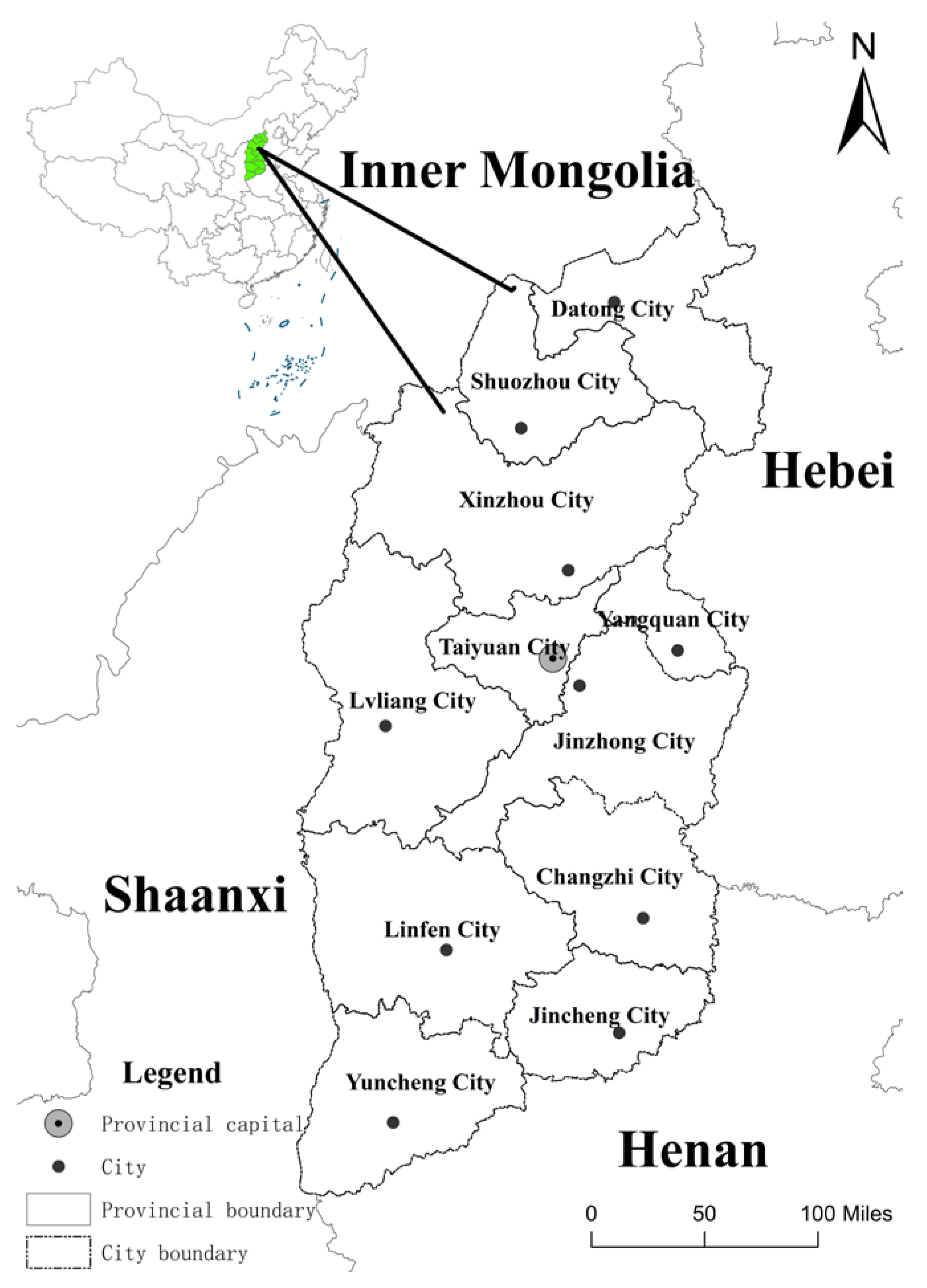
2.2. Study Area
2.3. Date Resources
3. Results and Analysis
3.1. Stationarity Test
3.2. The Determination of the Optimal Lag Order
3.3. Co-Integration Test
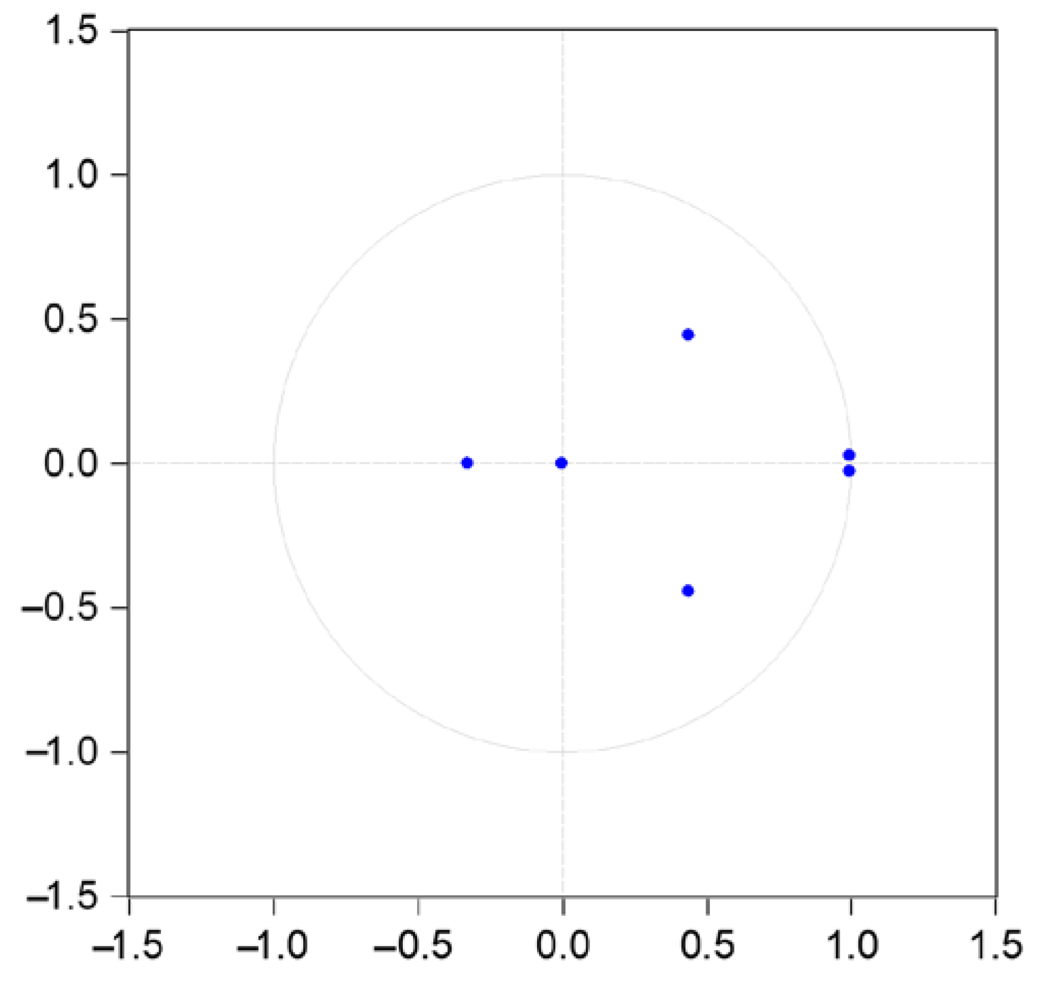
3.4. The VAR Model of CE, EG, and UR
3.5. Mutual Influence and Trend
4. Discussion
5. Conclusions
Author Contributions
Funding
Institutional Review Board Statement
Informed Consent Statement
Data Availability Statement
Conflicts of Interest
References
- UNFCCC. The Paris Agreement [EB/OL]. 2015. Available online: https://unfccc.int/process-and-meetings/the-paris-agreement/the-parisagreement (accessed on 12 September 2020).
- IPCC. Special Report: Global Warming of 1.5 °C [R/OL]. 2018. Available online: https://www.ipcc.ch/sr15/ (accessed on 12 September 2020).
- Xinhuanet. Full Text of Xi’s Statement at the General Debate of the 75th Session of the United Nations General Assembly [EB/OL]. 2020. Available online: http://www.xinhuanet.com/2020-09/22/c_1126527652.htm (accessed on 5 October 2020).
- Bei, A.; Weiwei, C.; Jing, G.; Cheng, S. Breaking a new blueprint and opening a new journey: Written on the occasion of the Fifth Plenary Session of the 19th CPC Central Committee. J. Friends Party Memb. 2020, 10, 8–11. [Google Scholar]
- Meyerson Frederick, A.B.; Merino, L.; Durand, J. Migration and environment in the context of globalization. Front. Ecol. Environ. 2007, 5, 182–190. [Google Scholar] [CrossRef] [Green Version]
- Guo, X.J.; Dong, S.; Wang, G.; Lu, C. Emergy-based urban ecosystem health evaluation for a typical resource-based city: A case study of Taiyuan, China. Appl. Ecol. Environ. Res. 2019, 17, 15131–15149. [Google Scholar] [CrossRef]
- Li, Y.; Wu, W.; Liu, Y. Evolution of Global Major Disasters During Past Century and Its Enlightenments to Human Resilience Building. Bull. Chin. Acad. Sci. 2020, 35, 345–352. [Google Scholar]
- Liu, Y.M. Respect for Nature is not a Beautiful Word. China Science Daily, 20 February 2020. [Google Scholar]
- Tongwu, X. Global health security: Threats, challenges and responses. China Int. Strategy Rev. 2019, 2, 87–104. [Google Scholar]
- Steinhauser, G.; Brandl, A.; Johnson, T.E. Comparison of the chernobyl and fukushima nuclear accidents: A review of the environmental impacts. Sci. Total Environ. 2014, 470–471, 800–817. [Google Scholar] [CrossRef] [PubMed]
- Grossman, G.M.; Krueger, A.B. Environmental Impacts of North American Free Trade Agreement; NBER Working Paper No.3914; National Bureau of Economic Research, Inc.: New York, NY, USA, 1991. [Google Scholar]
- Selden, T.; Song, D. Environmental Quality and Development: Is There a Kuznets Curve for Air Pollution Emissions. Environ. Manag. 1994, 27, 147–162. [Google Scholar] [CrossRef]
- Martinez, Z.I.; Bengochea-Morancho, A. Pooled Mean Group Estimation of An Environmental Kuznets Curve for CO2. Econ. Lett. 2004, 82, 121–126. [Google Scholar] [CrossRef]
- Karagoz, S.; Bakirci, K. Sustainable energy development in Turkey. Energ. Source Part B 2009, 5, 63–73. [Google Scholar] [CrossRef]
- Kaygusuz, K. Energy for sustainable development: A case of developing countries. Renew Sust. Energ. Rev. 2012, 16, 1116–1126. [Google Scholar] [CrossRef]
- Changsong, L. The Theoretical basis and policy Orientation of low-carbon development in China. Econ. Res. Ref. 2017, 40, 51–55. [Google Scholar] [CrossRef]
- Department of Trade and Industry UK. Our Energy Future: Creating A Low Carbon Economy; Energy White Paper; The Stationery Office: London, UK, 2003. [Google Scholar]
- Nerini, F.F.; Sovacool, B.; Hughes, N.; Cozzi, L.; Cosgrave, E.; Howells, M.; Tavoni, M.; Tomei, J.; Zerriffi, H.; Milligan, B. Connecting climate action with other Sustainable Development Goals. Nat. Sustain. 2019, 2, 674–680. [Google Scholar] [CrossRef]
- Limei, S.; Feng, X. A review of the research on the carbon emission based on Cite Space and construction of research system. Ecol. Sci. 2021, 40, 183–194. [Google Scholar]
- Rogelj, J.; Popp, A.; Calvin, K.V.; Luderer, G.; Emmerling, J.; Gernaat, D.; Fujimori, S.; Strefler, J.; Hasegawa, T.; Marangoni, G.; et al. Scenarios towards limiting global mean temperature increase below 1.5 °C. Nat. Clim. Chang. 2018, 8, 325–332. [Google Scholar] [CrossRef]
- Van Vuuren, D.P.; Stehfest, E.; Gernaat, D.E.H.J.; Berg, M.V.D.; Bijl, D.L.; De Boer, H.S.; Daioglou, V.; Doelman, J.C.; Edelenbosch, O.Y.; Harmsen, M.; et al. Alternative pathways to the 1.5 °C target reduce the need for negative emission technologies. Nat. Clim. Chang. 2018, 8, 391–397. [Google Scholar] [CrossRef]
- Grubler, A.; Wilson, C.; Bento, N.; Boza-Kiss, B.; Krey, V.; McCollum, D.; Rao, N.D.; Riahi, K.; Rogelj, J.; de Stercke, S.; et al. A low energy demand scenario for meeting the 1.5 °C target and sustainable development goals without negative emission technologies. Nat. Energy 2018, 3, 515–527. [Google Scholar] [CrossRef]
- Alam, M.M.; Murad, M.W.; Nornanc, A.H.M.; Ozturk, I. Relationships among carbon emissions, economic growth, energy consumption and population growth: Testing Environmental Kuznets Curve hypothesis for Brazil, China, India and Indonesia. Ecol. Indic. 2016, 70, 466–479. [Google Scholar] [CrossRef]
- Yaqing, W.; Deming, T.; Jiatian, Z.; Nan, M.; Baolong, H.; Zhiyun, O. Panel data analysis of the relationship between urban development and energy carbon emissions in China. Acta Ecol. Sin. 2020, 40, 7897–7907. [Google Scholar]
- Han, C.; Lining, W.; Wenying, C. Modeling on building sector’s carbon mitigation in China to achieve the 1.5 °C climate target. Energy Effic. 2018, 12, 483–496. [Google Scholar] [CrossRef]
- Jiang, K.; He, C.; Xu, X.; Jiang, W.; Xiang, P.; Li, H.; Liu, J. Transition scenarios of power generation in China under global 2 °C and 1.5 °C targets. Glob. Energy Interconnect. 2018, 4, 477–486. [Google Scholar] [CrossRef]
- Haikun, W.; Rongrong, Z.; Jun, B. Urban Carbon Emission Accounting in China—A case study of Wuxi city. China Environ. Sci. 2011, 31, 1029–1038. [Google Scholar]
- Bilgili, F.; Kocak, E.; Bulut, U.; Kuloğlu, A. The impact of urbanization on energy intensity: Panel data evidence considering cross-sectional dependence and heterogeneity. Energy 2017, 133, 242–256. [Google Scholar] [CrossRef]
- Wang, S.; Li, G.; Fang, C. Urbanization, economic growth, energy consumption, and CO2 emissions: Empirical evidence from countries with different income levels. Renew. Sustain. Energy Rev. 2018, 81, 2144–2159. [Google Scholar] [CrossRef]
- Asumadu-Sarkodie, S.; Owusu, P.A. Carbon dioxide emission, electricity consumption, industrialization, and economic growth nexus: The Beninese case. Energy Sources Part B Econ. Plan. Policy 2016, 11, 1089–1096. [Google Scholar] [CrossRef]
- Zhang, C.; Lin, Y. Panel estimation for urbanization, energy consumption and CO2 emissions: A regional analysis in China. Energy Policy 2012, 49, 488–498. [Google Scholar] [CrossRef]
- Adebayo, T.S.; Akinsola, G.D.; Odugbesan, J.A.; Olanrewaju, V.O. Determinants of environmental degradation in Thailand: Empirical evidence from ARDL and wavelet coherence approaches. Pollution 2021, 7, 181–196. [Google Scholar]
- Odugbesan, J.A.; Aghazadeh, S. Environmental Pollution and Disaggregated Economic Policy Uncertainty: Evidence from Japan. Pollution 2021, 7, 749–767. [Google Scholar]
- Adebayo, T.S.; Awosusi, A.A.; Odugbesan, J.A.; Akinsola, G.D.; Wong, W.K.; Rjoub, H. Sustainability of energy-induced growth nexus in Brazil: Do carbon emissions and urbanization matter? Sustainability 2021, 13, 4371. [Google Scholar] [CrossRef]
- Huo, T.; Xu, L.; Feng, W.; Cai, W.; Liu, B. Dynamic scenario simulations of carbon emission peak in China’s city-scale urban residential building sector through 2050. Energy Policy 2021, 159, 112612. [Google Scholar] [CrossRef]
- Haque, M.M.; Biswas, J.C.; Maniruzzaman, M.; Hossain, M.B.; Islam, M.R. Water management and soil amendment for reducing emission factor and global warming potential but improving rice yield. Paddy Water Environ. 2021, 19, 517–527. [Google Scholar] [CrossRef]
- Quan, C.; Cheng, X.; Yu, S.; Ye, X. Analysis on the influencing factors of carbon emission in China’s logistics industry based on LMDI method. Sci. Total Environ. 2020, 734, 138473. [Google Scholar] [CrossRef]
- Zheng, C.; Zhang, H.; Cai, X.; Chen, L.; Liu, M.; Lin, H.; Wang, X. Characteristics of CO2 and atmospheric pollutant emissions from China’s cement industry: A life-cycle perspective. J. Clean. Prod. 2021, 282, 124533. [Google Scholar] [CrossRef]
- Chontanawat, J.; Wiboonchutikula, P.; Buddhivanich, A. An LMDI decomposition analysis of carbon emissions in the Thai manufacturing sector. Energy Rep. 2020, 6, 705–710. [Google Scholar] [CrossRef]
- Adebayo, T.S.; Odugbesan, J.A. Modeling CO2 emissions in South Africa: Empirical evidence from ARDL based bounds and wavelet coherence techniques. Environ. Sci. Pollut. Res. 2021, 28, 9377–9389. [Google Scholar] [CrossRef]
- Ulucak, R.; Erdogan, F.; Bostanci, S.H. A STIRPAT-based investigation on the role of economic growth, urbanization, and energy consumption in shaping a sustainable environment in the Mediterranean region. Environ. Sci. Pollut. Res. 2021, 28, 55290–55301. [Google Scholar] [CrossRef]
- Xu, F.; Huang, Q.; Yue, H.; He, C.; Wang, C.; Zhang, H. Reexamining the relationship between urbanization and pollutant emissions in China based on the STIRPAT model. J. Environ. Manag. 2020, 273, 111134. [Google Scholar] [CrossRef]
- Majeed, M.T.; Tauqir, A. Effects of urbanization, industrialization, economic growth, energy consumption, financial development on carbon emissions: An extended STIRPAT model for heterogeneous income groups. Pak. J. Commer. Soc. Sci. 2020, 14, 652–681. [Google Scholar]
- Lu, Z.D. Impact of Urbanization on Carbon Emissions in China. Forum Sci. Technol. China 2011, 7, 134–140. [Google Scholar] [CrossRef]
- Hu, L.; Wang, J. Analysis of Long—term Effect and Short—term Fluctuation Effect of Urbanization on Carbon Dioxide Emissions in China. J. Arid. Land Resour. Environ. 2016, 30, 94–100. [Google Scholar]
- Zhang, X.; Li, M.; Li, Q.; Chen, Y.W.W. Threshold Effect of Urbanization on Carbon Emissions and Regional Spatial Distribution. Environ. Sci. Technol. 2018, 41, 165–172. [Google Scholar]
- Xingju, Z.; Shaobo, L. Rethinking the environmental impact of the IPAT model. China Popul. Resour. Environ. 2016, 26, 61–68. [Google Scholar]
- York, R.; Rosa, E.A.; Dietz, T. Analytic tools for unpacking the driving forces of environmental impacts. Ecol. Econ. 2003, 46, 351–365. [Google Scholar] [CrossRef]
- Zhiming, X.; Kui, Y.; Leming, Z.; Panpan, Y. Research of long-run equilibrium between economic growth/energy transformation and CO2 emissions: An empirical study based on provincial panel data analysis. Theory Pract. Financ. Econ. 2017, 38, 113–118. [Google Scholar]
- Yuanyuan, H.; Jianyu, L.; Wang, Z.; Hejie, P.; Saiying, F. Calculation and prediction of carbon emission from industrial scale energy consumption in Changsha. Territ. Nat. Resour. Study 2017, 5, 46–50. [Google Scholar]
- Fang, S.; Cao, G. Modelling extreme risks for carbon emission allowances—Evidence from European and Chinese carbon markets. J. Clean. Prod. 2021, 316, 128023. [Google Scholar] [CrossRef]
- Wang, Q.; Wang, S. Preventing carbon emission retaliatory rebound post-COVID-19 requires expanding free trade and improving energy efficiency. Sci. Total Environ. 2020, 746, 141158. [Google Scholar] [CrossRef] [PubMed]
- Zhang, M.; Anaba, O.A.; Ma, Z.; Li, M.; Asunka, B.A.; Hu, W. Enroute to attaining a clean sustainable ecosystem: A nexus between solar energy technology, economic expansion and carbon emissions in China. Environ. Sci. Pollut. Res. 2020, 27, 18602–18614. [Google Scholar] [CrossRef]
- Zhao, L.; Wen, F.; Wang, X. Interaction among China carbon emission trading markets: Nonlinear Granger causality and time-varying effect. Energy Econ. 2020, 91, 104901. [Google Scholar] [CrossRef]
- Yansui, L.; Bin, Y.; Yang, Z. Urbanization, Economic Growth and Carbon Dioxide Emissions in China: A Panel Cointegration and Causality Analysis. J. Geogr. Sci. 2016, 26, 131–152. [Google Scholar]
- Wang, Q.; Su, M. Drivers of decoupling economic growth from carbon emission–an empirical analysis of 192 countries using decoupling model and decomposition method. Environ. Impact Assess. Rev. 2020, 81, 106356. [Google Scholar] [CrossRef]
- Yu, J.; Shao, C.; Xue, C.; Hu, H. China’s aircraft-related CO2 emissions: Decomposition analysis, decoupling status, and future trends. Energy Policy 2020, 138, 111215. [Google Scholar] [CrossRef]
- Yi, M. A great song from high. Ind. China 1996, 2, 46–47. [Google Scholar]
- Niu, L.; Wang, K. Research on safety supervision model of Shanxi group coal enterprises. Procedia Eng. 2012, 43, 499–505. [Google Scholar]
- Guo, X.; Zhang, Z.; Zhao, R.; Wang, G.; Xi, J. Association between coal consumption and urbanization in a coal-based region: A multivariate path analysis. Environ. Sci. Pollut. Res. 2018, 25, 533–540. [Google Scholar] [CrossRef] [PubMed]
- Chen, Z.H. About 700,000 hectares of land have been subsided in mining area. Outlook Newsweek 2004, 47, 30–31. [Google Scholar]
- Howard, R.B.; Schipper, L.; Anderson, B. The structure and trends and intensity of energy use: Trends in five OECD nations. Energy J. 1993, 14, 27–44. [Google Scholar] [CrossRef] [Green Version]
- Zhang, L.F. Research on Energy Supply and Demand Forecasting Model and Development Countermeasures in China; Capital University of Economics and Business: Beijing, China, 2006. [Google Scholar]
- Engle, R.F.; Granger, C.W.J. Co-integration and error correction: Representation, estimation and testing. Econometrica 1987, 55, 251–276. [Google Scholar] [CrossRef]
- Johansen, S. Likelihood-Based Inference in Cointegrated Vector Autoregressive Models; Oxford University Press: Oxford, UK, 1995. [Google Scholar]
- Hendry, D.F. Dynamic Econometrics; Oxford University Press: Oxford, UK, 1995. [Google Scholar]
- Mabrouki, M. The sense of causality between growth and economic development: An essay on VAR modeling in the case of Tunisia. J. Smart Econ. Growth 2017, 2, 81–93. [Google Scholar]
- Bataa, E.; Vivian, A.; Wohar, M. Changes in the relationship between short-term interest rate, inflation and growth: Evidence from the UK, 1820–2014. Bull. Econ. Res. 2019, 71, 616–640. [Google Scholar] [CrossRef] [Green Version]
- Singh, K.; Vashishtha, S. Does any relationship between energy consumption and economic growth exist in India? A var model analysis. OPEC Energy Rev. 2020, 44, 334–347. [Google Scholar] [CrossRef]
- Anetor, F.O. Foreign direct investment inflows and real sector: A vector autoregressive (VAR) approach for the Nigerian economy. J. Dev. Areas 2019, 53, 3. [Google Scholar] [CrossRef]
- Barari, M.; Kundu, S. The role of the federal reserve in the us housing crisis: A var analysis with endogenous structural breaks. J. Risk Financ. Manag. 2019, 12, 125. [Google Scholar] [CrossRef] [Green Version]
- Mestl, H.E.S.; Aunan, K.; Fang, J.; Seip, H.M.; Skjelvik, J.M.; Vennemo, H. Cleaner production as climate investment—Integrated assessment in Taiyuan City, China. J. Clean. Prod. 2005, 13, 57–70. [Google Scholar] [CrossRef]
- Cole, M.A.; Rayner, A.J.; Bates, J.M. The environmental Kuznets curve: An empirical analysis. Environ. Dev. Econ. 1997, 2, 401–416. [Google Scholar] [CrossRef]
- Wang, Q.; Su, M. The effects of urbanization and industrialization on decoupling economic growth from carbon emission—A case study of China. Sustain. Cities Soc. 2019, 51, 101758. [Google Scholar] [CrossRef]
- Chen, L.; Liang, G.; Yi, X.; Feng, S.; Hengxu, Z. Forecasting and analysis of global carbon emissions in the context of energy transition based on econometrics. Glob. Energy Internet 2020, 3, 51–58. [Google Scholar]
- Shi, P.H.; Wu, P. Preliminary Estimation of Energy Consumption and CO2 Emissions from Tourism in China. Acta Geogr. Sin. 2011, 66, 235–243. [Google Scholar]


| Variable | N | Minimum | Maximum | Mean | Standard Deviation | Variation |
|---|---|---|---|---|---|---|
| UR | 40 | 0.21 | 0.63 | 0.38 | 0.13 | 0.02 |
| EG | 40 | 121.70 | 17,651.90 | 4952.04 | 5577.25 | 31,105,760.68 |
| CE | 40 | 3047.81 | 26,524.34 | 13,136.11 | 7891.11 | 62,269,634.69 |
| Variable | Test Type | t Statistic | Significance Level Critical Value | p | Verdict | ||
|---|---|---|---|---|---|---|---|
| 1% | 5% | 10% | |||||
| CE | Augmented Dickey–Fuller | −2.030489 | −4.219126 | −3.533083 | −3.198312 | 0.5664 | unstable |
| Phillips–Perron | −1.678684 | −4.211868 | −3.529758 | −3.196411 | 0.7417 | unstable | |
| Dickey–Fuller GLS (ERS) | −2.175237 | −3.77 | −3.19 | −2.890000 | 0.0363 | stable | |
| ΔCE | Augmented Dickey–Fuller | −4.872899 | −4.219126 | −3.533083 | −3.198312 | 0.0018 | stable |
| Phillips–Perron | −4.729038 | −4.219126 | −3.533083 | −3.198312 | 0.0027 | stable | |
| Dickey–Fuller GLS (ERS) | −5.010148 | −3.77 | −3.19 | −2.890000 | 0 | stable | |
| EG | Augmented Dickey–Fuller | −0.152411 | −4.211868 | −3.529758 | −3.196411 | 0.992 | unstable |
| Phillips–Perron | −0.390432 | −4.211868 | −3.529758 | −3.196411 | 0.9845 | unstable | |
| Dickey–Fuller GLS (ERS) | −1.200646 | −3.77 | −3.19 | −2.89 | 0.2377 | unstable | |
| ΔEG | Augmented Dickey–Fuller | −4.886404 | −4.219126 | −3.533083 | −3.198312 | 0.0017 | stable |
| Phillips–Perron | −4.891815 | −4.219126 | −3.533083 | −3.198312 | 0.0017 | stable | |
| Dickey–Fuller GLS (ERS) | −4.988007 | −3.77 | −3.19 | −2.89 | 0 | stable | |
| UR | Augmented Dickey–Fuller | −0.547331 | −4.219126 | −3.533083 | −3.198312 | 0.9766 | unstable |
| Phillips–Perron | −0.842275 | −4.211868 | −3.529758 | −3.196411 | 0.9525 | unstable | |
| Dickey–Fuller GLS (ERS) | −1.57701 | −3.77 | −3.19 | −2.89 | 0.1246 | unstable | |
| ΔUR | Augmented Dickey–Fuller | −8.611742 | −4.219126 | −3.533083 | −3.198312 | 0 | stable |
| Phillips–Perron | −8.228623 | −4.219126 | −3.533083 | −3.198312 | 0 | stable | |
| Dickey–Fuller GLS (ERS) | −8.755748 | −3.77 | −3.19 | −2.890000 | 0 | stable | |
| Original Hypothesis | Eigenvalue | Trace Test | 0.05 Critical Value | p | Max-Eigen Test | 0.05 Critical Value | p |
|---|---|---|---|---|---|---|---|
| Hypothesis 1: None * | 0.393625 | 30.40582 | 29.79707 | 0.0425 | 18.50951 | 21.13162 | 0.1119 |
| Hypothesis 2: At most 1 | 0.268691 | 11.89632 | 15.49471 | 0.162 | 11.57799 | 14.2646 | 0.1275 |
| Hypothesis 3: At most 2 | 0.008566 | 0.318324 | 3.841466 | 0.5726 | 0.318324 | 3.841466 | 0.5726 |
| Dependent Variable | Excluded | Chi-Sq | df | Prob. | Null Hypothesis |
|---|---|---|---|---|---|
| CE | EG | 12.40813 | 2 | 0.002 | |
| UR | 3.513237 | 2 | 0.1726 | ||
| All | 13.27646 | 4 | 0.01 | ||
| EG | CE | 1.967703 | 2 | 0.3739 | |
| UR | 0.654709 | 2 | 0.7208 | ||
| All | 2.456159 | 4 | 0.6525 | ||
| UR | CE | 0.226869 | 2 | 0.8928 | |
| EG | 4.953261 | 2 | 0.084 | ||
| All | 8.409556 | 4 | 0.0777 |
Publisher’s Note: MDPI stays neutral with regard to jurisdictional claims in published maps and institutional affiliations. |
© 2022 by the authors. Licensee MDPI, Basel, Switzerland. This article is an open access article distributed under the terms and conditions of the Creative Commons Attribution (CC BY) license (https://creativecommons.org/licenses/by/4.0/).
Share and Cite
Zhang, Z.; Wang, G.; Guo, X. Long-Term and Short-Term Effects of Carbon Emissions on Regional Healthy Development in Shanxi Province, China. Sustainability 2022, 14, 5173. https://doi.org/10.3390/su14095173
Zhang Z, Wang G, Guo X. Long-Term and Short-Term Effects of Carbon Emissions on Regional Healthy Development in Shanxi Province, China. Sustainability. 2022; 14(9):5173. https://doi.org/10.3390/su14095173
Chicago/Turabian StyleZhang, Zhongwu, Guokui Wang, and Xiaojia Guo. 2022. "Long-Term and Short-Term Effects of Carbon Emissions on Regional Healthy Development in Shanxi Province, China" Sustainability 14, no. 9: 5173. https://doi.org/10.3390/su14095173
APA StyleZhang, Z., Wang, G., & Guo, X. (2022). Long-Term and Short-Term Effects of Carbon Emissions on Regional Healthy Development in Shanxi Province, China. Sustainability, 14(9), 5173. https://doi.org/10.3390/su14095173