Article

Decomposition and Decoupling Analysis of Carbon Emissions from Cultivated Land Use in China’s Main Agricultural Producing Areas

School of Public Policy and Administration, Nanchang University, Nanchang 330031, China
*
Author to whom correspondence should be addressed.
Sustainability 2022, 14(9), 5145; https://doi.org/10.3390/su14095145
Submission received: 4 April 2022 / Revised: 19 April 2022 / Accepted: 22 April 2022 / Published: 24 April 2022

Abstract

:
In-depth analysis of the decoupling state between cultivated land carbon emissions and cultivated land use factors can provide a basis for coordinating the relationship between food security and ecological environment. On the base of systematically calculating the carbon source of cultivated land, this paper calculated the carbon emission of cultivated land in China’s main agricultural production areas from 2000 to 2020, and explored its temporal and spatial pattern and evolution process. Then, using the LMDI decomposition method and the improved kaya identity, the factors affecting the carbon emissions of cultivated land are divided into five effects: structure, economy, technology, society and population, and then the Tapio decoupling theory is used to analyze the relationship between carbon emissions and these five effects. At the same time, to explore the further relationship between carbon emissions and cultivated land structure, we also studied the decoupling state between carbon emissions and the cultivated land area of 6 main crops. The results showed: during the study period, carbon emissions experienced three stages: fluctuating growth, accelerated growth and slow decline. In the most recent stage, structural, economic and population effects still have some impact on the carbon emissions of cultivated land, changes in cultivated land area where cotton, sugar and tobacco are planted will still affect its carbon emissions. To intervene, policy measures such as promoting the use of clean energy, increasing agricultural imports, and increasing carbon taxes for some industries can be considered.

1. Introduction

Food security has always been a major strategic issue related to the overall situation. China accounts for one-fifth of the world’s population and only 8% of the world’s cultivated land [1]. Food security faces multiple challenges. If the climate continues to warm in the medium and long term, it will seriously affect food production. According to China’s “National Population Development Plan (2016–2030)”, the population of China will reach 1.45 billion in 2030, and the food demand will be 484–609 million tons. Due to the huge demand for agricultural products, China must maintain a cultivated land utilization model characterized by high-intensity input of agricultural materials, but the environmental consequences that follow cannot be ignored: in planting, irrigation and other links, agricultural energy, chemical fertilizers, pesticides, agricultural film and other materials are important sources of carbon emissions, carbon emissions from cultivated land contribute to 17% of China’s carbon emissions [2]. Under the influence of the dual strategic pressure of “big grain concept” and “carbon neutrality”, it is necessary to rationally adjust China’s cultivated land use structure, grasp the bottom line of food security, and at the same time achieve the emission reduction target.
In the current research on food security and carbon emissions, the main consensus of scholars is “low carbon and high yield”, but each scholar has chosen different entry points. Some scholars focus on comparative studies in different regions, such as Yang constructed a global EBM model to estimate the grain production efficiency of 30 provinces and three functional areas in China from 2001 to 2018 by considering the net carbon sink and non-point source pollution emissions in grain production, the conclusion shows that compared with the high-efficiency provinces, the distribution liquidity is stronger, and the low-efficiency provinces have obvious “poverty traps”, and the vicious circle of low-level food development is not easy to break through [3]. Other scholars have paid attention to carbon sequestration in agriculture and carbon sequestration technologies, such as Yan studied the carbon emission characteristics of crop production and the important role of carbon sequestration, and concluded that if the import of agricultural products in China is not significantly affected, the carbon emission of crop production has already shown a peak trend [4]. In the policy research on the joint realization of food security and carbon emissions, some studies have shown that in the short term, agricultural operators should be encouraged to reasonably expand the scale of food production and improve the production efficiency of chemical inputs and machinery. In the long run, it is necessary to continue to popularize and promote green production technology, reduce the dependence of food production on chemicals, and gradually transform to a low-carbon production model [5]. In this article, we believe that the development of China’s rural areas, the use of cultivated land and the way it is used will change the food security situation from the perspective of food structure, and will also have a certain degree of impact on carbon emissions.
At present, the issue between carbon emissions and cultivated land use has received extensive attention from the academic community. Scholars’ research mainly focuses on the relationship between carbon emissions and the utilization efficiency of cultivated land resources [6,7], agricultural output value [8] and grain yield [9], and discusses the temporal and spatial characteristics [10] and influencing factors [11] of carbon emissions. At the same time, it also discusses the policy of economic compensation mechanism for cultivated land protection [12] and the improvement of cultivated land [13]. However, the issue of food security does not only represent the increase of agricultural output value or the improvement of production efficiency, but also involves the organization of the agricultural industry and the way of cultivated land use. The relationship between these and carbon emissions has rarely been paid attention to by scholars, and in our study, we not only included the change of cultivated land area as the main factor of the study, but also related to the main crops (such as grains, cotton, oil, sugar, tobacco, vegetables and fruits, etc.) to conduct subdivided research, in order to make recommendations for the adjustment of food structure under the dual pressures of carbon emissions and food security.
In the study of carbon emission related issues, various theoretical methods, such as ARIMA models [13], BP neural network [14] are widely used. However, decoupling analysis, which originated from the concept of physics, has become an important method of research, and it was originally applied to explain the reduction or absence of interrelationships between physical quantities [15]. Later, it was first introduced to research in the field of resources and environment of the Organization for Economic Cooperation and Development (OECD) in the 21st century [16]. There are then numerous studies using this approach to study the interrelationships between economic growth and energy consumption and GDP and the environment and resources. Among them, the log-mean-division exponential method (LMDI), as the most representative IDA decomposition method, performs the best due to the advantage of no residual decomposition. Therefore, it is considering to be the most accurate and practical method in the current decomposition system. Recently, this method is still widely used by scholars. For example, Chen used this method to study carbon dioxide emissions in the OECD [17]. Monika used this method to study the energy policies of EU countries [18]. In terms of land use, Guo also used this method to study the relationship between utilization land and economic growth [19]. The above studies have drawn reliable conclusions and have been widely recognized. However, few studies have been conducted on the relationship between cultivated land use and carbon emissions using this method. This paper mainly provides the following contributions to the relevant literature: (1) The current situation of cultivated land use in the study area is analyzed, and the influencing factors of cultivated land carbon emissions are decomposed using the LMDI model and the kaya identity; (2) Use the Tapio model to study the decoupling relationship between various factors in cultivated land use and carbon emissions; (3) The decoupling relationship between the planting area and carbon emissions of the main crops in cultivated land is studied in detail, and the results are expected to provide policy reference for the adjustment of grain structure.

2. Data and Methodology

2.1. Study Area

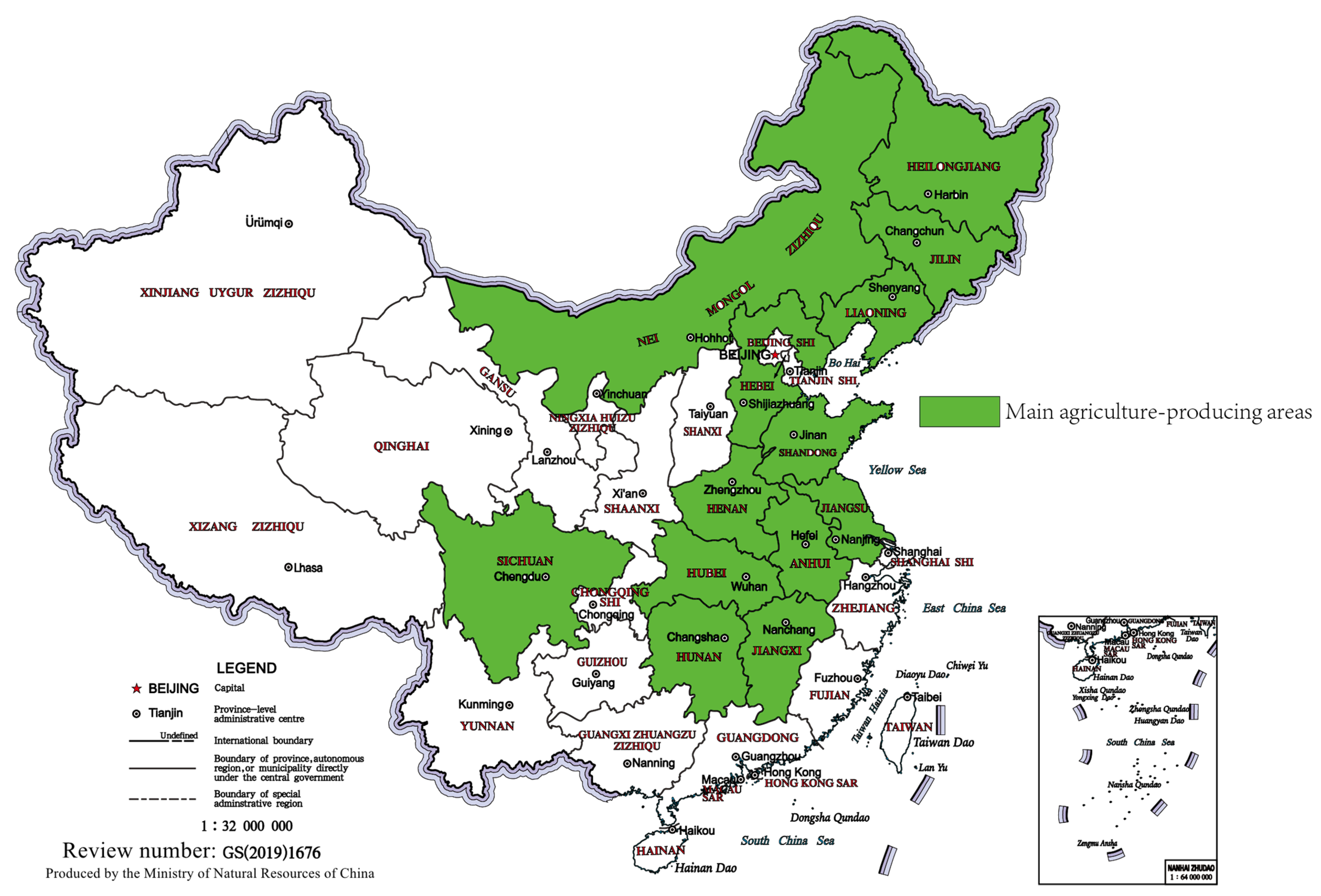
According to the “Opinions on Reforming and Improving Several Policies and Measures for Comprehensive Agricultural Development” promulgated by the Ministry of Finance, China’s main agricultural producing areas mainly include 13 provinces (Figure 1), which are important agricultural commodity production bases in China [20]. According to the data released by the “China Statistical Yearbook 2021”, the total cultivated land area of crops in these areas in 2020 is 116,063,400 hectares, accounting for 69.27% of China’s total cultivated land area, the effective irrigated area is 42,490,500 hectares, accounting for 61.44% of China’s total effective irrigated area, and the agricultural output value is 4373.49 billion yuan, accounting for 60.95% of China’s total agricultural output value. Meanwhile, the crops produced in these provinces are mainly used to meet China’s domestic demand, and the products produced in these areas account for about 80% of the total sales in China [21]. Therefore, studying the relationship between cultivated land carbon emissions and cultivated land use in this region is of great significance to China’s crop production security and agricultural economic stability in the future.

2.2. Cultivated Land Carbon Emission Accounting Method

At present, the academic worlds mainly believed that the carbon emission of cultivated land utilization is the carbon emission of cultivated land resource utilization is limited to the direct or indirect greenhouse gas carbon emission effect caused by human production activities in the process of cultivated land utilization [22]. The purpose of this paper is to provide ideas and references for the low-carbon policy of cultivated land use, and the low-carbon use of cultivated land is mainly manifested in the reduction of high-carbon material input and soil damage in the process of cultivated land utilization. Based on this, this paper believes that the carbon emissions from the utilization of cultivated land resources are mainly manifested as greenhouse gas emissions directly or indirectly caused by planting behaviors or farmers’ behaviors, and existing literatures have not yet formed a unified method for carbon emission measurement of cultivated land utilization. Based on IPCC carbon emission factor method, combined with the research results of Ding [10] and Xie [6], in the formula C represent the total carbon emissions during the use of cultivated land, Cj represents the quantity of carbon source produced by fertilizers, pesticides, agricultural plastic films, and the total power of agricultural machinery, plowing, and irrigation during the cultivated land use, and βj Indicates the carbon emission Coefficients, the calculation formula is as follows:
C = C j = ( C j × β j )
The carbon emission calculation formula and carbon emission coefficient table of cultivated land resource utilization are as Table 1.

2.3. LMDI Decomposition Analysis

To formulated the cultivated land use policy under the carbon neutrality goal, it is necessary to further clarify the influencing effects of cultivated land use after knowing the cultivated land utilization status in the region. Therefore, this paper adopts the improved Kaya identity and the LMDI decomposition method to explore the factors of cultivated land utilization, and it is expected to obtain the direction and specific impact of the influencing factors on the cultivated land use.
The Kaya identity was first proposed and named by Japanese professor Yoichi Kaya, which links the carbon dioxide produced by human activities with economic, policy, population and other factors to establish an identity relationship [23]. The LMDI analysis method proposed by ANG B.W. in 1998 allows for an additive full decomposition of the difference in carbon emissions [24]. This method can effectively solve the “zero value” problem and eliminate the impact of decomposition residuals [25] and is an effective tool to explore the factors influencing CO2 emissions. The LMDI method has been the most popular method of the IDA methods, this popularity will likely increase over time [17]. The LMDI method is an effective tool to explore factors affecting CO2 emissions. This paper aims to explore the factors that affect carbon emissions in the process of cultivated land use (the carbon emissions mentioned below all represent the cultivated land carbon emissions). Therefore, using the Kaya identity and the LMDI decomposition method, the CO2 emissions of the main agricultural producing areas in China are decomposed into the following forms, the calculation formula is as follows:
C = i C i L i × L Y × Y B × B P × P
A description of each variable in the Equation (2) is indicated in Table 2.
Set: C L i = C i L i ,   L Y = L Y .   Y B = Y B ,   B P = B P .
Equation (2) can be transformed into:
C = i C L i × L Y × Y B × B P × P
In Equation (3) CLi is the carbon emissions from panting the i-th crop, which represents the structural effect. The larger the CLi, the more carbon emissions from growing the i-th crop and the planting structure is more unfavorable for carbon emission reduction. LY is the cultivated land depletion caused by ten thousand RMB agriculture GDP, which represents the economic effect. The larger the LY, the more cultivated land is needed to achieve the goal of agricultural GDP and the lower the economic efficiency of cultivated land. YB is the output per unit of agricultural laborer, which represents the technical effect. The larger YB, the higher the technical level of agricultural production, the less manpower required by ten thousand RMB agriculture GDP. The BP is ratio of population involved in agricultural labor to population they supported, which represents the social effect. The larger BP is, the higher the agricultural participation of the society and the higher the degree of agricultural intensification in the study area. P is the population supported by agriculture in the study area, which represents the population effect. The larger P, the more pressure on agricultural supply, which may lead to an increase carbon emissions.
Under the addition decomposition method of LMDI, the change of C from a base year 0 and a target year T, represented by ΔC, and it can be decomposed into five effects as follows: (i) the changes in the structural effect (represented by ΔCCL); (ii) the changes in the economic effect (represented by ΔCLY); (iii) the changes in the technical effect (represented by ΔCYB); (iv) the change in the labor social effect (represented by ΔCBP), and (v) the changes in the population effect (represented by ΔCP), as shown in Equation (4).
ΔC = CTC0 = ΔCCL + ΔCLY + ΔCYB + ΔCBP + ΔCP
Each effect in the right-hand side of Equation (4) can be expressed as follows:
Δ C C L = i L ( C i T , C i 0 ) × ln ( C L i T C L i 0 )
Δ C L Y = i L ( C i T , C i 0 ) × ln ( L Y T L Y 0 )
Δ C Y B = i L ( C i T , C i 0 ) × ln ( Y B T Y B 0 )
Δ C B P = i L ( C i T , C i 0 ) × ln ( B P T B P 0 )
Δ C P = i L ( C i T , C i 0 ) × ln ( P T P 0 )
Here, L ( C i T , C i 0 ) = C i T C i 0 ln C i T ln C i 0 , ( C i T C i 0 ) .

2.4. Decoupling Analysis

In 1993, the OECD [26] first proposed the concept of “decoupling”, which described the relationship between economic driving factors and environmental pressure factors, and divided the decoupling relationship into two states: absolute decoupling and relative decoupling, in which absolute decoupling represented economic growth and resource consumption remained unchanged or negatively increased, the relative decoupling showed that the economic growth rate was faster than that of resource consumption. However, the OECD decoupling model has obvious defects. Firstly, it has high sensitivity to the base period and end-of-period values of variables, which is prone to calculation bias. Secondly, the classification of decoupling relationship types is too general and cannot subdivide the relationship between economic growth and environmental pressure [27]. In 2005, Tapio [28] further proposed the concept of “decoupling elasticity” based on the OECD decoupling model, which refers to the ratio of economic growth rate to the degree of change in carbon emission, which can better reflect the sensitivity of changes in carbon emissions to economic growth. According to the value of decoupling elasticity, TAPIO defines 8 decoupling states, namely expansive negative decoupling, strong negative decoupling, weak negative decoupling, weak decoupling, strong decoupling, weak decoupling, expansive coupling and recessive coupling, (Table 3 presents eight grades corresponding to decoupling elasticity).
Therefore, based on this theory and Equations (4)–(9), the decoupling elastic indexes between carbon emission intensity of the five effects can be illustrated as:
ε C C L = Δ C / C 0 Δ C L / C L 0 = ( Δ C L + Δ L Y + Δ Y B + Δ B P + Δ P ) / C 0 Δ C L / C L 0 = δ C / δ C L
ε C L Y = Δ C / C 0 Δ L Y / L Y 0 = ( Δ C L + Δ L Y + Δ Y B + Δ B P + Δ P ) / C 0 Δ L Y / L Y 0 = δ C / δ L Y
ε C Y B = Δ C / C 0 Δ Y B / Y B 0 = ( Δ C L + Δ L Y + Δ Y B + Δ B P + Δ P ) / C 0 Δ Y B / Y B 0 = δ C / δ Y B
ε C B P = Δ C / C 0 Δ B P / B P 0 = ( Δ C L + Δ L Y + Δ Y B + Δ B P + Δ P ) / C 0 Δ B P / B P 0 = δ C / δ B P
ε C P = Δ C / C 0 Δ P / P 0 = ( Δ C L + Δ L Y + Δ Y B + Δ B P + Δ P ) / C 0 Δ P / P 0 = δ C / δ P
Here, εCL, εLY, εYB, εBP, εP denotes decoupling elasticity index of carbon emissions and structural effect, economic effect, technical effect, social effect and population effect, respectively. δCL, δLY, δYB, δBP, δP represent the growth rate of structural effect, economic effect, technical effect, social effect and population effect, respectively.
According to the Tapio, the decoupling elasticity index between carbon emissions and cultivated land can be illustrated as:
ε C A = Δ C / C 0 Δ L / L 0 = ( C T C 0 ) / C 0 ( L T L 0 ) / L 0 = δ C / δ L
ε C A i = Δ C i / C i 0 Δ L i / L i 0 = ( C i T C i 0 ) / C i 0 ( L i T L i 0 ) / L i 0 = δ C i / δ L i
Here, εCA denotes decoupling elasticity index of carbon emissions and total cultivated land area. δC and δL represent the growth rate of carbon emission and total cultivated land area from a base year 0 to a target year T, ΔL represent the change area of cultivated land. εCAi denotes decoupling elasticity index of carbon emissions and total cultivated land area planting the i-th crop, δLi represent the growth rate of the cultivated land area planting the i-th crop from a base year 0 to a target year T. ΔLi represent the change area of cultivated land planting the i-th crop.

2.5. Data Source

China’s main agricultural producing areas include the following 13 provinces: Heilongjiang, Jilin and Liaoning in Northeast China; Hebei, Inner Mongolia in North China Area; Shandong, Jiangsu and Anhui in East China Area; and Henan, Hunan, Hubei and Jiangxi in Central China Area. In the China Central Economic Work Conference held at the end of December 2013, it was mentioned that these 13 provinces are responsible for more than 75% of China’s grain output, more than 80% of commercial grain, and more than 85% of the annual increase in demand for grain comes from these 13 provinces. It can be said that these 13 provinces bear the largest agricultural output and the greatest pressure on agricultural resources. Although other provinces also undertake a part of agricultural labor, according to the total comparison of factors such as yield level, sown area and labor force structure, among these 13 provinces, agriculture has almost reached its yield limit [29]. Therefore, we believe that the research on these 13 provinces will be more representative, and can conduct research on some urgent problems in China’s agriculture. To calculate carbon emissions, the data of fertilizer scalar volume, pesticide usage, agricultural plastic film usage, total power of agricultural machinery, crop sown area and effective irrigation area during the planting process of each type crops in each province is from the “China Rural Statistical Yearbook 2001–2021”, the data range is 2000–2020. The data of cultivated land area, agricultural GDP and Chinese population are from “China Statistical Yearbook 2001–2021”, the data range is 2000–2020. The data of population of agricultural is from Statistical yearbooks 2001–2021 for provinces in the study area, the data range is 2000–2020.

3. Results and Analysis

3.1. Changes in Carbon Emissions and Agriculture GDP

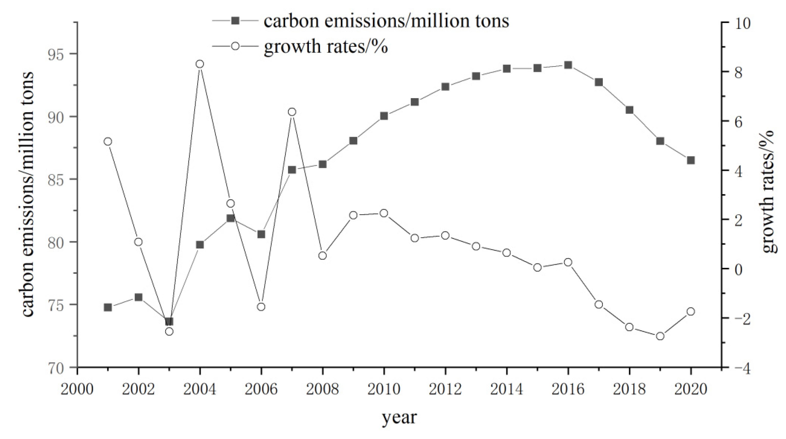
Figure 2 describes the cultivated land carbon emissions and growth rates of China’s main agricultural producing areas, calculated by the Equation (1). As seen in Figure 1, carbon emission of cultivated land has increased by 19.33 million tons (25.85%) from 2001 to 2016. This may be due to the increase in the input of agricultural materials such as chemical fertilizers, pesticides, agricultural films and agricultural machinery or the degree of soil damage caused by agrochemical and mechanization. This conclusion can be confirmed by the results of data calculation. According to the coefficients in Table 1, it can be seen that the carbon emissions from agricultural irrigation, farming and other behaviors accounted for only 0.18% and 1.48% of the total carbon emissions of cultivated land on average from 2000 to 2020, and the use of agricultural machinery and fertilizer application accounted for 13.31% and 41.44%, respectively. It can be seen that these factors have a significant impact on cultivated land carbon emissions. At the same time, carbon emissions from agricultural diesel were 6.66 million tons at the end of 2000, peaked at 15.23 million tons at the end of 2016, and dropped to 8.85 million tons at the end of 2020. At the end of 2000, the carbon emission from chemical fertilizer application in cultivated land was 28.69 million tons, reached a record high of 40.16 million tons by the end of 2016, and dropped to 34.91 million tons by the end of 2020. However, after 2009, the growth rate of cultivated land carbon emissions gradually declined slightly, especially after 2016, it entered a negative growth stage, which indicates that the cultivated land carbon emissions in the study area were declined rapidly. In only three years, from 2016–2019, the carbon emissions of cultivated land was dropped from 9.41 to 8.80 million tons, down by 6.44%. It indicates that China has achieved some positive results with regards to carbon emissions reduction in recent years. It is worth noting that, the growth rate of carbon emissions from2019 to 2020 was increased slightly, which may indicate that the growth rate of carbon emissions will change from the rapid decline state to a stable state in the future.
The annual change in carbon emissions was calculated in Microsoft Excel and the results are shown in Table 4. As it indicates that in the period of 2000–2005, the carbon emissions from grain cultivation fluctuated widely, and in the period of 2015–2020, the carbon emissions from grain and vegetable & fruit cultivation fluctuated widely, and other types of carbon emissions changes are relatively stable. Overall, the change of carbon emissions in the study area still mainly comes from the carbon emissions change of grain cultivation.
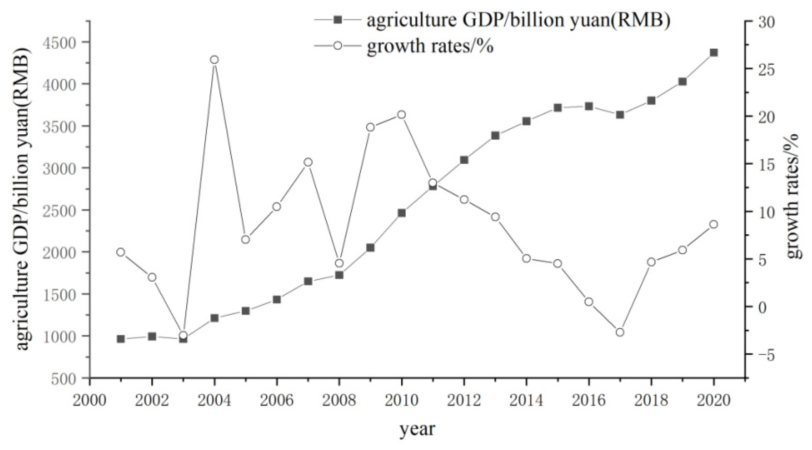
As shown in Figure 3, from 2001 to 2020, the agriculture GDP in China’s main agricultural producing areas was generally on the rise. In 2001, the agriculture GDP was only 963 billion yuan (RMB), and in 2020, the agriculture GDP has risen to 4373.49 billion yuan (RMB), with an increase of 354.15%. From 2010 to 2017 the agriculture GDP growth slowed, but picked up after 2017.
From 2000 to 2016, carbon emissions and agriculture GDP increased, and from 2017 to 2020, carbon emissions decreased while the agriculture GDP was still increasing. This indicates that changes in carbon emissions and the agriculture GDP were not consistent in recent years. It is demonstrated that carbon emissions reduction can be achieved without sacrificing agriculture economic growth in China’s main agricultural producing areas in recent years. Wu et al. [9] have drawn similar conclusions in their studies. That’s means carbon emissions from cultivated land use and economic benefits was possible to achieve a win-win situation.

3.2. Changes in Crop Areas

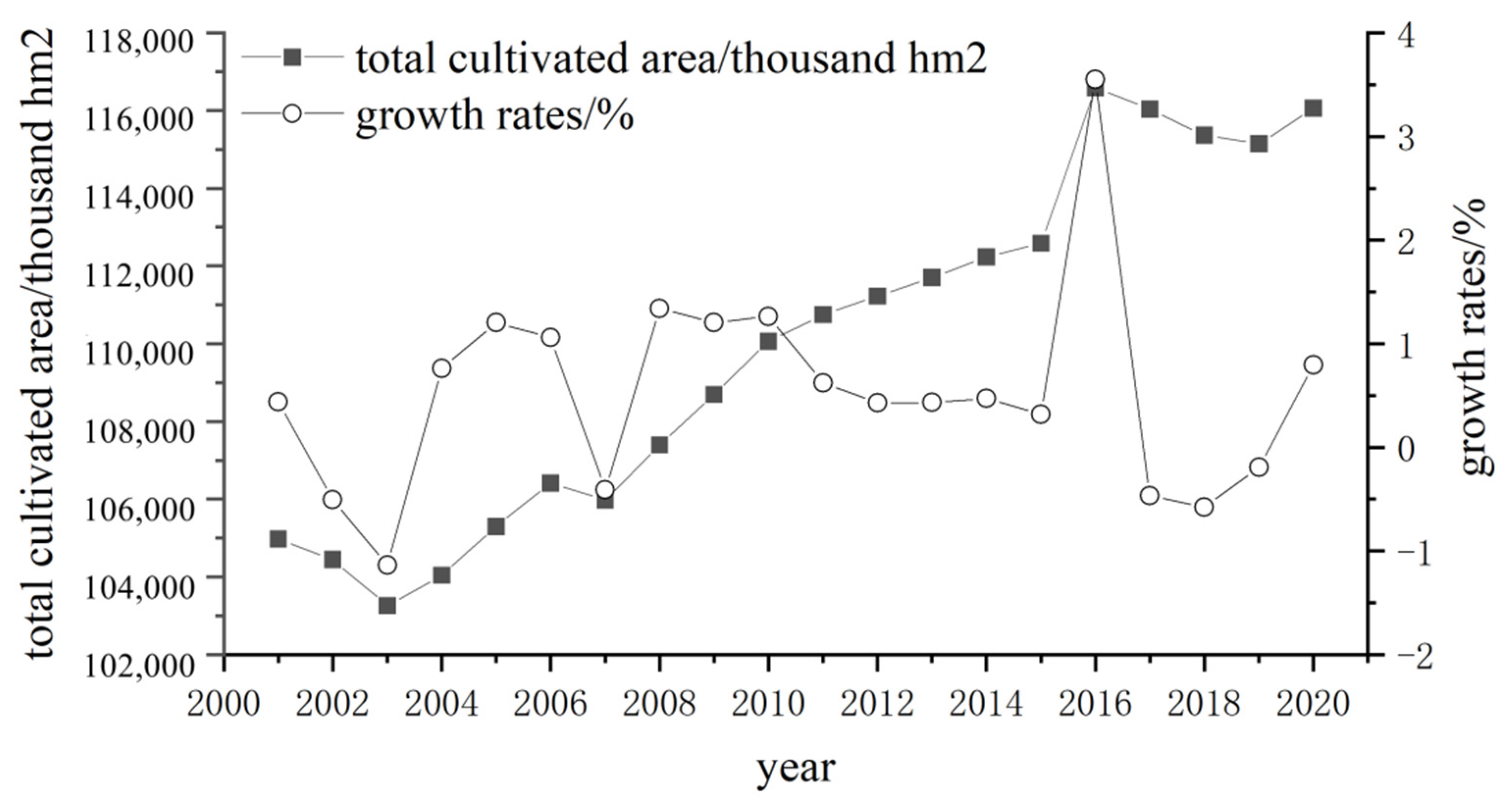
Figure 4 describes the changes of the total cultivated land area (here it is expressed in terms of crops sown area) in China’s main agricultural producing areas during 2001–2020. As shown in Figure 4, the area of cultivated land in the study area has increased by 11,090 thousand hm2 (10.56%) from 2001 to 2020. Compared with the growth of agricultural GDP shown in Figure 3, it’s indicated that the agricultural production efficiency in the study area has been greatly improved in these years. From 2003 to 2015, the cultivated land area was in a state of steady growth, in 2016 the cultivated area has increased by 3998 thousand hm2 (3.55%), and from 2016 to 2020 the cultivated land area has not much volatility and keep it around an average of 115,840.04 hm2.
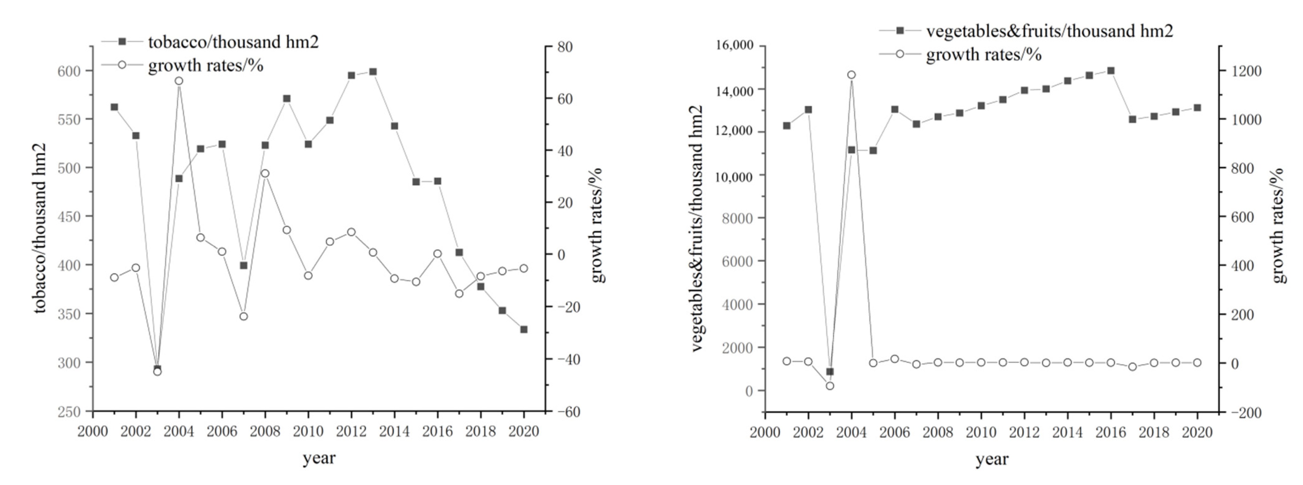
Figure 5 describes the changes of 6 main types of crop sown area. It is worth noting that the difference between the total cultivated land area and the sum of the sown area of the 6 main crops is represents “the others” sown area, since “the others” types and sown areas cannot be accurately counted, they are not shown in the figure. As shown in Figure 5, the sown area of grain was in a state of consistent growth while the sown area of cotton was in a state of decreasing. The sown area of oil (seeds) and tobacco leaves fluctuates greatly. The sown area of sugar, vegetables & fruits are relatively stable except for individual years that fluctuate greatly. As can be seen from the figure, from 2003 to 2005 the growth rates of 6 each main type of crops have a large fluctuations, this indicates that in these few years, the plating industry structure in the study area has been greatly adjusted. This coincides with the time when carbon emissions increased significantly in Figure 2, and at the same time, the growth rate of agricultural GDP has also increased significantly after 2003 (Figure 3). This proves that the adjustment of the plating industry structure was stimulated the agricultural GDP, improved cultivated land use efficiency but increased carbon emissions. This is consistent with the relevant research drawn by B. Kuang, et al. [30] on China’s cultivated land and carbon emissions. Fortunately, in recent years, although the structure of the plating industry has not been greatly adjusted compared with 2003–2005, with carbon emissions have been controlled. Therefore, maintaining this structure of the plating industry will have a positive impact on further carbon emissions control and the development of a low-carbon agricultural economy.
The annual change in cultivated land area was calculated in Microsoft Excel and the results are shown in Table 5. As it indicates that the change of total cultivated land area and total carbon emissions are basically consistent, and this trend is also reflected in every major crop. This shows that the carbon emissions produced by planting different crops are not very different. Thus, take the ratio of carbon emissions and cultivated land area planting in each type of crop (represented by CCL) as the structural effect and the ratio of cultivated area and agriculture GDP (represented by CLY) as the economic effect, they can reflect the impact of planting structure on carbon emissions and the impact of economic efficiency of agricultural production on carbon emissions respectively.

3.3. Changes in Population and Number of Agricultural Laborer

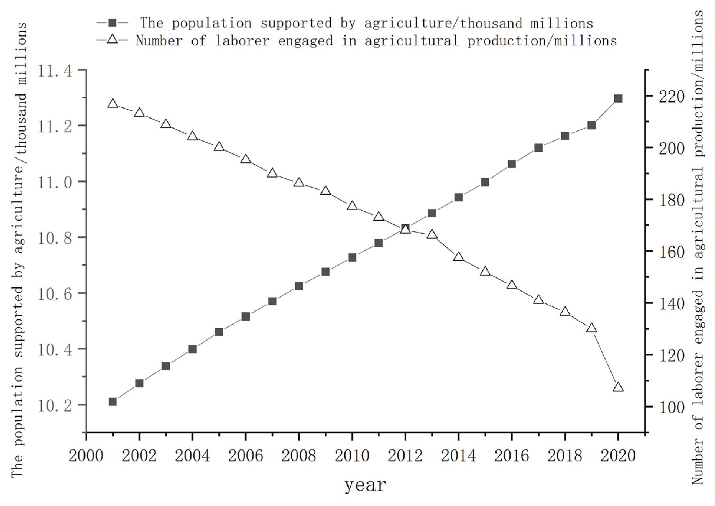
Figure 6 describes the trend of changes in the population supported by the agricultural in the study area from 2001 to 2020. As seen in Figure 6, the population rose almost in a straight line during this period, increasing from 10.21 thousand million in 2001 to 11.30 thousand million in 2020, with an increase of 10.64% and an average annual growth rate of 0.54%. However, the number of laborer engaged in agriculture production kept a plummeting trend from 2001 to 2020, decreasing from 216.60 million in 2001 to 107.15 million in 2020, with a drop of 50.53% and an average annual reduction rate of 3.45%. Take the ratio of agriculture GDP and the number of agriculture labor can reflect the technical effect to carbon emission (represented by CYB). While the area of cultivated land and the population supported by agriculture kept increasing trend, the number of laborer engaged in agriculture continued to decrease, it is clearly proved the improvement of agricultural technology, especially in 2009–2020, the gap between the population and the number of agricultural laborer increased widened significantly. In this case, it is worth exploring that whether the reduction in the number of laborer willing to engaged in agriculture can also force the development of agricultural technology. Based on the above analysis, we take this factor as one of the effects (represented by CBP) of cultivated land carbon emission, and this is also an unavoidable problem when discussing the social benefit of cultivated land use [31].
Summarizing the above data description, it can be seen that according to the change data of carbon emissions in 2000–2020, the carbon emissions can be divided into three stages, namely: the shock rise period (2000–2007), the uniform rise period (2007–2016) and slow decline period (2016–2020). During these three periods, the agricultural GDP in the study area showed a slow increase, a decelerated increase and an accelerated increase, while the total cultivated land area showed a fluctuating increase, a rapid increase and remained stable. From 2000 to 2020, the planting area of 6 main food crops was dominated by grain and maintained an upward trend, while the sown area of cotton was in a state of decreasing, the sown area of oil(seeds) and tobacco leaves fluctuates greatly and the sown area of sugar, vegetables & fruits are relatively stable except for individual years that fluctuate greatly. In terms of population, in the past 20 years, while the total population has risen steadily, the number of people engaged in agricultural labor is slowly declining.

3.4. Effects of All Factors on Changes in Carbon Emissions

According to the analysis in Section 3.1, we can divide the changes in carbon emissions into three periods: 2000–2007, 2007–2016, 2016–2020. According to the decomposition results of LMDI, through the calculation of Equations (4)–(9), the effects of the influencing factors on changes in carbon emissions during these three periods were calculated and the results are shown in Table 6.
As shown in Table 6, from 2000 to 2007, the carbon emissions increased by 14.63 million tons. The carbon emissions reduced by economic effect, and population effect were 45.34 and 14.58 million tons, respectively. While the carbon emissions increased by structural effect, technical effect and social effect were 13.55, 57.75 and 3.25 million tons, respectively. As evident, between 2000 and 2007, carbon emissions were most affected by economic and technical effects.
Between 2007 and 2016, carbon emissions increased by 8.36 million tons. Among them, the growth caused by technical effect and population effect was 96.53 and 4.08 million tons respectively. However, affected by structural effect, economic effect, and social effects, carbon emissions decreased by 0.21, 64.81 and 27.23 million tons respectively. Therefore, carbon emissions were most affected by economic and technical effects during this period.
Between 2016 and 2020, carbon emissions decreased by 7.60 million tons. The reductions in carbon emissions due to structural effect, economic effect and social effect were 7.19, 14.67 and 30.23 million tons, respectively. During this period, carbon emissions increased by 42.59 and 1.90 million tons only due to technical effect and population effect. It can be seen that between 2016–2000, carbon emissions were most affected by technical and social effects.
Overall, between 2000 and 2020, carbon emissions increased by 15.40 million tons. Among them, economic and technical effects have the greatest impact, technical effect increase carbon emissions, while economic effect reduce carbon emissions. The influence of these two effects tends to become smaller as time goes by, and the influence of structural effect is changing from positive to negative.
To assessing the impact of each effect on carbon emissions in more detail, the decomposition analysis results of each year are listed in Table 7.
For a clearer observation, the impact of each effect on carbon emissions is listed in Figure 7, in the form of a percentage bar graph.
As can be seen from Table 7 and Figure 7, technical effect has the most impact on increasing carbon emissions, it accounts for 36–49% of the incremental contribution to carbon emissions most of the time. Particular in 2015–2016 and 2016–2017, the contribution rate of technical effect was only 27% and 13%. And in 2002–2003, the contribution rate of technical effect was even −13%, resulting in a reduction of 0.75 million tons of carbon emissions. Economic effect was the greatest contributor to reducing carbon emissions most of the time. Economic effect is the effect that contribute the most to reducing carbon emissions, except for the low contribution rate in 2019–2020, which was only 13%, even in 2002–2003, 2015–2016 and 2016–2017 caused carbon emissions to increase by 1.45, 2.83 and 2.13 million tons, the rest of the time the contribution rate was between 21% and 42%. The contribution rate of social effect to the reduction of carbon emissions tends to increase year by year, except in 2002–2003, the contribution rate once reached 35% (resulting in a reduction of 2 million tons of carbon emissions), and in recent years, it is almost between 28–34%. The impact of structural effect on carbon emissions has gradually turned from positive to negative, in 2015–2016, its contribution rate even reached 22% (a decrease of 3.03 million tons of carbon emissions). The impact of population effect on carbon emissions is small and relatively stable.
To sum up, whether it is divided into three periods or analyzed year by year, the conclusions are generally consistent. That is, technical effect has the greatest impact on carbon emissions, followed by economic and social effect, and the impact of structural effect has gradually changed from increase to decrease, and there is an expanding trend, the impact of population effect is small and stable.

3.5. Decoupling Analysis Results

According to the decoupling analysis method listed in Table 3, the decoupling relationship between carbon emissions and various effects decomposed by LMDI decomposition method, as well as the decoupling relationship between carbon emissions and cultivated land area can be judged.

3.5.1. Decoupling State of Each Effect

Through the calculation of Equations (3)–(13), the decoupling elasticity of the effects affecting cultivated land carbon emissions can be obtained. The decoupling status can be obtained by querying Table 3. The decoupling elasticity is listed in Table 8, and the decoupling status is listed in Table 9.
It can be seen from Table 8 that from 2000 to 2020, the decoupling elasticity of carbon emissions and cultivated land structure is very close to 0 and is positive most of the time, indicating that the two are positively correlated in most times. This is mainly due to the fact the overall cultivated land area kept increasing in this period. Before 2007, carbon emissions and structural effect showed a situation of weak decoupling (WD) and weak negative decoupling (WND) alternated. From 2007 to 2016, they showed a shift from weak decoupling (WD) to strong negative decoupling (SND). After 2016, the performance of structural effects became stable in the weak negative decoupling (WND) state. This shows that there is always a certain correlation between carbon emissions and structural effects, but the degree of correlation is not obvious. To further explore the driving effect of cultivated land structure on carbon emissions and explore ways to improve this state, we will discuss the decoupling state of carbon emissions and cultivated land area in more depth in Section 3.5.2.
In 2000–2020, the elasticity between carbon emissions and economic effect (i.e., the cultivated land consumed per billion yuan of agricultural GDP) was negative for most of the time, as carbon emissions generally realized an overall increasing trend, while the economic effect is decreasing in this period, so the decoupling state between carbon emissions and economic effect is mainly a strong negative decoupling (SND). But from 2016, they gradually lost this relationship and turned into a weak negative decoupling (WND) or strong decoupling (SD) state, which shows that since this time, carbon emissions always subject to some influence from economic effect. And from the absolute value of the decoupling elasticity, this relationship still has an increasing trend, which is more obvious in 2017–2019.
The technical effect represents the economic amount produced by each agricultural laborer. The decoupling elasticity between carbon emissions and technical effects is always close to 0 and is positive most of the time. From 2000 to 2016, the relationship between carbon emissions and technical effect nearly remained weak decoupling (WD), after 2016 entered a strong decoupling (SD). This shows that agricultural technology has improved, which is what we want, but we would prefer to see a reduction in carbon emissions at the same time. In recent years, the decoupling state of carbon emissions and economic effects has always been, while carbon emissions still maintain an upward trend, which shows that technical effect is not the main effect affecting cultivated land carbon emissions changing, and may continue to do so in the future.
The ratio between agricultural laborers and the number of people they support reveals participation in agricultural labor and represents social effect. The decoupling elasticity between carbon emissions and social effect was mainly negative before 2016 and positive after that, and the absolute value keeps increasing. This means that people’s willingness to participate in agricultural labor is decreasing while carbon emissions are generally on the rise. After 2016, the decoupling state between carbon emissions and social effect also changed from strong negative decoupling (SND) to weak negative decoupling (WND). Before 2016, the growth rates of carbon emissions and social effect were both on the rise, and the relationship between the two was weak and negative decoupling. However, after 2016, the growth rate of carbon emissions slowed down, and the two became strong decoupling, which shows that the growth of society’s willingness to engage in agricultural labor can reduce the driving effect of carbon emissions.
Before 2007, the decoupling elasticity between agricultural carbon emissions and population effect showed an unstable state and the absolute value of elasticity is closer to 0.5. From 2007 to 2016, this state changed to a weak decoupling (WD), indicating that since 2007, the number of population driving changes in carbon dioxide emissions to some extent. But after 2016, the decoupling elasticity value between the two became negative, and the absolute value is increasing, which led to the decoupling state showing strong decoupling (SD). This suggests that the population’s impact on carbon emissions has generally been slowly decreasing, with almost unrelated in recent years.
To determine the main effects of carbon emissions, the average decoupling elasticity of each effect at each stage is listed in Table 10.
As can be seen from Table 10, in 2000–2007, only the values of εYB and εP were the closest to 1, which means that during this period, the driving effect of technical and population on carbon emissions was the most obvious. From 2007 to 2016, the influence of technical effect and population effect gradually declined, while the impact of economic and social effects on carbon emissions was increasing. In 2016–2020, the driving role effect on carbon emissions becomes the economic effect and social effect, while the impact of technical and population effects will continue to weaken. In general, the driving role of technological effect and population effect on carbon emissions was declined, while the impact of economic and social effects continued to get stronger. The overall impact of structural effect on carbon emissions does not change much. To further explore the driving role of land structure on carbon emissions, we will conduct a more in-depth discussion in Section 3.5.2.
In summary, population effect, technical effect and population effect have a certain driving effect on the change of cultivated land carbon emissions. Among them, the population effect is the most significant but keeps decreasing. Economic and social effects did not show obvious left and right in the past but have shown in recent years. Therefore, to follow the development trend in recent years, the focus on controlling carbon emissions should be shifted to structural, economic and social effects.

3.5.2. Decoupling State of Carbon Emissions and Cultivated Land Area

Substitute the data in Table 4 and Table 5 into Equations (15) and (16), the decoupling elasticity of carbon emissions and cultivated land area can be calculated and the decoupling state can be judged. The calculation results of the decoupling elasticity are listed in Table 11, and the judging results of the decoupling state are listed in Table 12.
As can be seen from Table 12, before 2007, the decoupling status of several indicators in the table showed obvious instability. The main reason is that in 2000–2007, although carbon emissions showed an upward trend, their growth rates fluctuated greatly, resulting in large changes in the numerators in Equations (15) and (16).
At this stage of 2007–2016, since the growth rate of cultivated land is far less than the growth rate of carbon emissions, DC,L continuously presented the state of expansive negative decoupling (END) in 2008–2014, and εCA > 1.2, indicated that the total cultivated area of the study area is driving the change in carbon emissions to some extent. However, in the periods of 2007–2008 and 2014–2016, the decoupling elasticity remained positive but 0 < εCA < 0.8, DC,L showed a weak decoupling (WD) state, indicating that the growth rate of carbon emissions was smaller than the growth rate of cultivated land area, and the changes in cultivated land area during this period also led to changes in carbon emissions, but the driving effect was far less pronounced than during 2008–2014. The relationship between grain planting area and its carbon emissions and the relationship between total area and total carbon emissions generally show a relatively consistent trend of change. The decoupling elasticity of carbon emissions in cotton planting and its cultivated land area is 0.8 < εCA2 < 1.2 in most of the time, and the decoupling state shows a recessive coupling (RC), which shows that both the growth rate of carbon emissions and the cultivated land area are decreasing in the cotton planting area, and the change of carbon emission is almost completely affected by the cultivated land area. The absolute value of εCA3, which represents the decoupling elasticity of oil planting areas, is mostly greater than 1.2 during this period, indicating that the carbon emission and of cultivated land area is far less than the carbon emissions, when the growth rate of carbon emissions is negative, the decoupling state is mostly realized as strong decoupling (SD), and when growth rate of carbon emissions is positive, it shows expansion negative decoupling (END) or strong negative decoupling (SND), which indicates that carbon emissions are less affected by cultivated land area in oil planting areas. The absolute value of εCA4, which represents the elasticity of carbon emissions in sugar planting area and its cultivated land area, is always greater than 0 but has a gradually decreasing trend, and its decoupling state DC,L4 also gradually changed from expansive coupling (EC) or recessive coupling (RC) to weak decoupling (WD), this shows that the impact of carbon emissions by planting area in sugar planting areas is gradually weakening. The absolute value of εCA5, which represents the elasticity between tobacco planting area, is greater than 0 and 0.8 < εCA5 < 1.2 in most of the time, and its decoupling state DC,L5 is mostly shown as expansive coupling (EC) or recessive coupling (RC), this shows that carbon emissions in tobacco growing areas are closely related to their growing areas. εCA6 represents the elasticity in the vegetable and fruit planting area, during 2007–2013, the overall change trend was similar to εCA, and its decoupling state was also similar, but in 2013–2016, the absolute value of the decoupling elasticity became smaller and closer to 1, and the decoupling state became expansive coupling (EC), but due to the obvious downward trend of the decoupling elasticity, it quickly changed to a strong decoupling (SD) state after that, this shows that carbon emissions from vegetable and fruit cultivation is affected by the area of cultivated land, which has experienced a process of gradually increasing but then decreasing rapidly.
In the stage of 2016–2020, the decoupling elasticity value and decoupling state of each indicator basically tend to be stable. DC,L, DC,L1, and DC,L6 are gradually changing to a strong decoupling (SD) state, which indicates that in general, the change in carbon emissions is less affected by the area of cultivated land, and carbon emissions are unbound from change in the planting area of grains and vegetables and fruits. DC,L2, DC,L3 and DC,L5 gradually changed from coupling to decoupling, indicating that in the planting areas of cotton, oil and tobacco, carbon emissions are gradually less affected by the area of cultivated land. However, the relationship between carbon emissions and the area of cultivated land in the sugar planting area is still in a large fluctuation.
To judge the main effects of carbon emissions under the change of cultivated land area in the three stages, the average value of the decoupling elasticity in the three stages is listed in Table 13.
As can be seen from Table 13, in 2000–2007, only the average of εCA2 of the decoupling elasticity had an absolute value between 0.8 and 1.2, it shows that the change in carbon emissions has the highest correlation with the cotton planting area during this period. In 2007–2016, the absolute value of the average of εCA4, εCA5 and εCA6 were between 0.8–1.2, which indicates that the change in carbon emissions during this period is closely related to the planting area of sugar, tobacco, vegetables and fruits. In 2016–2000 only absolute values of the average of εCA2 was between 0.8 and 1.2, which means that carbon emissions were most affected by cotton planting area during this period. Overall, only the absolute values of the average of εCA1 and εCA2 were between 0.8 and 1.2, indicating that during the study period, change in carbon emissions were greatly affected by changes in grain and cotton planting area.
In summary, the change of carbon emissions is gradually reduced by the change in cultivated land area. Generally speaking, it is most affected by the changes in the areas of cotton planting, and this trend has not been improved in recent years. In 2007–2016, the correlation between carbon emission changes and cultivated land area changes was higher, and the effects of changes in sugar and tobacco planting areas were greater than in other periods, but after 2016, these effects were moderately weakened.
4. Conclusions and Suggestions for Policy Makers

4.1. Conclusions

In this paper, the LMDI decomposition method and the Kaya identity framework are used to decompose the factors affecting cultivated land carbon emissions, and the influencing effects driving cultivated land carbon emissions from 2000 to 2020 are divided into five: structural effect, economic effect, technological effect, social effect and population effect. Then, the Tapio decoupling analysis method is used to analyze the impact of cultivated land carbon emissions and structural effect, economic effect, technological effect, social effect and population effect on carbon emission increments, as well as the decoupling elasticity, and the decoupling state is obtained. In addition, this paper decomposes the plant types of cultivated land, and substitutes the carbon emissions and planting area of the six types of plants into the Tapio model for analysis to explore the contribution of each crop to the increase in carbon emissions of cultivated land during the production process.
The results of the study can be summarised as follows.
First, according to the change trend and growth rate data of cultivated land carbon emissions from 2000 to 2020, the change of carbon emissions can be divided into three stages: 2000–2007 is the fluctuation period, 2007–2016 is the growth period, 2016–2020 is the emission reduction period. In these three periods, among the five effects decomposition by LMDI method (structure, economy, technology, society and population), the positive effect of technical effect is the largest, while the negative effect of economic effect is the largest. The negative effect of social tends to increase, and the positive effect of population is always small. Among them, the structural effect gradually turns from positive to negative over time, and in the third stage, the negative effect it brings has been very significant. The technical effect represents the agricultural GDP per labor engaged in agriculture. With the improvement of technical means, the output will of course be higher, and with the increase in the use of mechanical technology, carbon emissions will inevitably increase. On the contrary, the reduction in the cultivated land area used to produce every 1 billion yuan of agricultural GDP also brings about a decrease in carbon emissions, which shows that the increase in agricultural output can reduce carbon emissions. At the same time, the reduction of people’s willingness to engage in agricultural labor will obviously reduce the carbon emissions of cultivated land. All the above are in line with theories related to economics and management, and the impact of structural effects cannot be clearly analyzed through panel data, and needs to be further discussed in the decoupling analysis.
Second, through the decoupling analysis of the Tapio model,, in the first stage, the factors affecting carbon emissions are mainly structural effect, technical effect and population effect. This relationship tends to be stable in the second stage, but in the third stage, the effects affecting carbon emissions have become structural effect, economic effect and social effect, while technical effect and population effect have shown a state of strong decoupling. At the same time, after decomposing the cultivated land structure, we used the Tapio model to decouple it again and found that in the cultivated land planting structure, cotton planting has the greatest impact on carbon emissions, while the impact of sugar planting has increased in the third stage, and the impact of tobacco planting has gradually declined and has almost decoupled in the past two years. The decoupling results show that the adjustment of agricultural technology has not been as effective as before on carbon emissions in recent years, while changing the area of cultivated land (attention should be paid to the planting area of cotton, sugar and tobacco), optimizing the structure of agricultural production, and adjusting people’s willingness to engage in agricultural production should be the main interventions in cultivated land carbon emissions.

4.2. Suggestions for Policy Makers

4.2.1. Promote the Use of Clean Energy and Increase Agricultural Imports

In China’s main agricultural producing areas, the carbon emissions of cultivated land and the structure of cultivated land, agricultural economic development and population have not yet been decoupled, while the carbon emissions caused by technological effects are the most, but due to the strong decoupling effect, it is not easy to control. Based on the above conclusions, to control the carbon emission of cultivated land in China’s main agricultural producing areas, it is necessary to promote the use of clean energy in agricultural machinery, irrigation and other high-energy-consuming machinery while adjusting the agricultural industrial structure. At the same time, it can also be considered to increase the import of agricultural products to reduce the pressure on agricultural production caused by the population.

4.2.2. Focus on Industries That Are Highly Related to Carbon Emissions, Increase Carbon Tax, and Promote Low-Carbon Development

At present, in the cultivated land producing cotton, sugar and tobacco leaves in China’s main agricultural production areas, the carbon emissions and the expansion of cultivated land have not been decoupled. Especially the production of sugar, which has contributed more and more to the increase in carbon emissions in recent years. Therefore, in the next adjustment of the agricultural industry structure, the pressure of emission reduction must be take into account, such as incorporating a higher carbon tax into these industries, such as to establish a policy model with optimal output, structure and emission reduction effect. At the same time, priority should be given to improving green and clean technologies in the cultivation of these three types of crops, improving waste disposal methods, and promoting the transformation of cultivated land use to low carbon.

4.3. Future Perspectives

The conclusions showed that to achieve carbon emission reduction in cultivated land, China should give more consideration to cooperation and imports with other countries, and due to the current complex international situation, food security has received widespread attention, especially in a country with a large agricultural and population like China. In China, some top journals have begun to solicit manuscripts on food security from the academic community, which shows that in the current form, research on food security needs urgent attention and innovation. At the same time, after China’s commitment to carbon neutrality, the technological development of various industries is inevitably constrained by the use of energy. We only studied the relationship between food security and carbon emissions from the perspective of cultivated land. Under the dual pressures of food security and carbon neutrality in the future, how will China or other regions in the world choose a development model? The impact of food security and carbon emissions may become a hot topic of future research.
Our next research will focus on the cooperation and synergy between various regions in China, such as the synergy between energy utilization, or the synergy in the distribution of agricultural product output, to further study the measures for simultaneous governance of food security and carbon emissions.

Author Contributions

Resources, C.F.; Writing—original draft, W.M.; Writing—review & editing, H.L. All authors have read and agreed to the published version of the manuscript.

Funding

China National Social Science Foundation Annual Project: Research on the Path and Supporting Policies of Agricultural Non-point Source Pollution Control in Poyang Lake Basin (18BGL187); Major Bidding Issues for the Base of the Ministry of Education of China: Research on the Competitiveness of Green Development in Central China Based on the Coordinated Perspective (18JJD790006).

Institutional Review Board Statement

Not applicable.

Informed Consent Statement

Not applicable.

Data Availability Statement

Not applicable.

Conflicts of Interest

The authors declare no conflict of interest.

References

  1. Chen, S.; Xu, J.T.; Zhang, H.P. The impact of climate change on grain production in China: An empirical analysis based on county-level panel data. Chin. Rural. Econ. 2016, 5, 2–15. (In Chinese) [Google Scholar]
  2. Li, B.; Zhang, J.B.; Li, H.P. Spatial and temporal characteristics of China’s agricultural carbon emissions and decomposition of influencing factors. China Popul. Resour. Environ. 2011, 21, 80–86. [Google Scholar]
  3. Yang, Q.; Si, X.H.; Wang, J. Measurement and Distribution Dynamic Evolution of China’s Grain Production Efficiency under the Target of Emission Reduction and Increase in Remittance. J. Nat. Resour. 2022, 37, 600–615. (In Chinese) [Google Scholar]
  4. Yan, S.J.; Deng, A.X.; Shang, Z.Y.; Tang, Z.W.; Chen, C.Q.; Zhang, J.; Zhang, W.J. Characteristics of carbon emissions from crop production in my country and the carbon emission reduction and carbon sequestration pathways for carbon neutralization. J. Crops 2022, 48, 930–941. (In Chinese) [Google Scholar]
  5. Yang, C.; Hu, P.Q.; Diao, B.D.; Cheng, J.H.; Cui, H.Y. Environmental Performance of Policies in Main Grain Producing Areas: Based on the Perspective of Agricultural Carbon Emissions. China Popul. Resour. Environ. 2021, 31, 35–44. [Google Scholar]
  6. Xie, H.L.; Zhang, Y.W.; Choi, Y.R. Measuring the Cultivated Land Use Efficiency of the Main Grain-Producing Areas in China under the Constraints of Carbon Emissions and Agricultural Nonpoint Source Pollution. Sustainability 2018, 10, 1932. [Google Scholar] [CrossRef] [Green Version]
  7. Niu, H.P.; Zhang, A.L.; Li, M.Q. Reconstruction of farmland utilization benefit system and economic compensation mechanism for farmland protection. Res. Agric. Mod. 2009, 3, 164–167. [Google Scholar]
  8. Tian, Y.; Zhang, J.B.; Li, B. Spatial-temporal characteristics and decoupling elasticity of carbon emissions from agricultural land use in Hubei Province. Yangtze River Basin Resour. Environ. 2012, 21, 1514–1519. (In Chinese) [Google Scholar]
  9. Wu, H.Y.; Huang, H.J.; Chen, W.K. Research on the decoupling effect of carbon emissions from cultivated land use and grain production in China’s main grain producing areas. Geogr. Geo-Inf. Sci. 2021, 6, 13. [Google Scholar]
  10. Ding, B.G.; Yang, S.W.; Zhao, Y.; Yi, S. Decoupling and Decomposition Analysis of and decoupling effect of carbon emissions from the utilization of cultivated land resources in China. China Land Sci. 2019, 33, 45–54. [Google Scholar]
  11. Zhang, P.Y.; Qin, M.Z.; Yan, J.H.; Li, J.; Yang, L.; Sun, C. Analysis of Influencing Factors and Characteristics of Cultivated Land Resource Utilization Benefit in Henan Province. China Popul. Resour. Environ. 2013, 3, 162–169. [Google Scholar]
  12. Luo, X.; Ao, X.H.; Zhang, Z.; Wan, Q.; Liu, X.J. Spatiotemporal variations of cultivated land use efficiency in the Yangtze River Economic Belt based on carbon emission constraints. J. Geogr. Sci. 2020, 30, 535–552. [Google Scholar] [CrossRef]
  13. Lv, J.Y.; Du, J.N.; Cao, M.; Fan, X.F. Carbon emissions trading price prediction using ARIMA-SVM model. J. Xi’an Univ. Sci. Technol. 2020, 40, 542–548. [Google Scholar]
  14. Zhao, C.B.; Mao, C.M. Prediction of China’s carbon emission intensity based on the combined model of Arima and BP neural network. Yangtze River Basin Resour. Environ. 2012, 6, 665–671. [Google Scholar]
  15. Ning, Y.; Zhang, B.; Ding, T.; Zhang, M. Analysis of regional decoupling relationship between energy-related CO2 emission and economic growth in China. Nat. Hazards 2017, 87, 867–883. [Google Scholar] [CrossRef]
  16. Organization for Economic Co-Operation and Development (OECD). Sustainable Development: Indicators to Measure Decoupling of Environmental Pressures from Economic Growth. 2002. Available online: http://www.oecd.org/officialdocumentspublicdisplaydocumentpdf/?cote=sg/sd(2002)1/final&doclanguage=en (accessed on 15 October 2002).
  17. Chen, J.D.; Wang, P.; Cui, L.B.; Shuo, H.; Song, M.L. Decomposition and decoupling analysis of CO2 emissions in OECD. Appl. Energy 2018, 231, 937–950. [Google Scholar] [CrossRef]
  18. Monika, P.; Stawomir, S.; Katarzyna, F. The role of energy policy on the decoupling processes in the European Union countries. J. Clean. Prod. 2021, 10, 10. [Google Scholar]
  19. Guo, S.; Wang, Y.; Huang, J.; Dong, J.; Zhang, J. Decoupling and Decomposition Analysis of Land Natural Capital Utilization and Economic Growth: A Case Study in Ningxia Hui Autonomous Region, China. Int. J. Environ. Res. Public Health 2021, 18, 646. [Google Scholar] [CrossRef]
  20. Jiang, L.; Zhu, F.S. Food Production Status and Policy Suggestions in Main Production Areas of China. Agric. Econ. 2015, 36, 17–24. [Google Scholar]
  21. Jiang, H.P.; Wu, Z.P. The Policy Suggestions on Establishing Grain Transfer Area for Transferring Payment in Main Production Areas. China Dev. Obs. 2009, 12, 24–25. (In Chinese) [Google Scholar]
  22. Li, K.Q.; Chen, J.J.; Ma, D.D. Growth mechanism and trend prediction of farmland input carbon emissions in Hunan Province based on STIRPAT and GM (1,1) models. River Basin Resour. Environ. 2018, 27, 345–352. (In Chinese) [Google Scholar]
  23. Kaya, Y. Impact of Carbon Dioxide Emission on GNP Growth: Interpretation of Proposed Scenarios; Paper Presented to IPCC Energy and Industry Subgroup, Response Strategies Working Group; IPCC: Paris, France, 1990. [Google Scholar]
  24. Ang, B.W.; Zhang, F.Q.; Choi, K.H. Factorizing changes in energy and environmental indicators through decomposition. Energy 1998, 23, 489–495. [Google Scholar] [CrossRef]
  25. Ang, B.W. LMDI decomposition approach: A guide for implementation. Energy Policy 2015, 86, 233–238. [Google Scholar] [CrossRef]
  26. OECD. Indicators to Measure Decoupling of Environmental Pressure from Economic Growth; OECD: Paris, France, 2002. [Google Scholar]
  27. Sun, Y.H.; Li, Z.M. The Decoupling Relationship between Economic Development and Carbon Emissions in China’s Provinces Research. China Popul. Resour. Environ. 2011, 21, 87–92. [Google Scholar]
  28. Tapio, P. Towards a theory of decoupling: Degrees of decoupling in the EU and the case of road traffic in Finland between 1970 and 2001. J. Transp. Policy 2005, 12, 137–151. [Google Scholar] [CrossRef] [Green Version]
  29. Jiang, H.P. Five major problems to be solved urgently in the main grain producing areas. China Dev. Obs. 2014, 7, 33–34. [Google Scholar]
  30. Bing, K.G.; Xin, H.L.; Min, Z.B.; Dan, L.C. Provincial cultivated land use efficiency in China: Empirical analysis based on the SBM-DEA model with carbon emissions considered. Technol. Forecast. Soc. Chang. 2020, 151, 119874. [Google Scholar]
  31. Pang, Y.; Zhang, J.J.; Ye, Y.G. Research on the utilization efficiency of cultivated land resources in China. China Popul. Resour. Environ. 2004, 5, 34–38. [Google Scholar]
Figure 1. Location of China’s main agricultural producing areas. (Note: This map is based on the standard map with the approval number GS (2019) 1676 issued by the Standard Map Service Website of the Ministry of Natural Resources of China, the base map has not been modified.).
Sustainability 14 05145 g001
Figure 2. Cultivated land carbon emissions and growth rates of China’s main agricultural producing areas (2001–2020).
Sustainability 14 05145 g002
Figure 3. Agriculture GDP and growth rates of China’s main agricultural producing areas (2001–2020).
Sustainability 14 05145 g003
Figure 4. Total cultivated land area and growth rates of China’s main agricultural producing areas (2001–2020).
Sustainability 14 05145 g004
Figure 5. 6 main types of crop sown area and growth rates of China’s main agricultural producing areas (2001–2020).
Sustainability 14 05145 g005aSustainability 14 05145 g005b
Figure 6. The population of agricultural supported and number of laborer engaged in agricultural production in the study area (2001–2020).
Sustainability 14 05145 g006
Figure 7. Contributions of all effect to carbon emissions in each year.
Sustainability 14 05145 g007
Table 1. Carbon emission coefficient of cultivated land utilization.
Carbon SourceCarbon Source Input/UnitCarbon Emission Coefficient
Fertilizer (C1)Fertilizer scalar volume/kg0.8956 (kg/kg)
Pesticide (C2)Pesticide usage/kg4.9341 (kg/kg)
Agricultural plastic film (C3)Agricultural plastic film usage/kg5.18 (kg/kg)
Agricultural machinery power (C4)Total power of agricultural machinery/kW0.5927 (kg/kw)
Plowing (C5)Crop sown area/hm23.126 (kg/hm2)
Irrigation (C6)Effective irrigation area/hm220.5 (kg/hm2)
Table 2. Variable descriptions.
VariableDefinition
CTotal CO2 emissions (million tons)
CiCarbon emissions from the production of the i-th crop (million tons)
LTotal cultivated land(here it is expressed in terms of crops sown area) (thousand hm2)
LiSown area of the i-th crop (thousand hm2)
Yagriculture GDP, here represents the GDP of the planting industry (billion yuan in RMB)
BNumber of laborer engaged in agricultural production (millions)
PThe population of agricultural supported in the study area (thousand million)(According to Jiang’s research [2], the number of the study areas‘ agricultural supported is 80% of the entire Chinese population)
(Note: The crops in the study area are divided into 6 main types: grain, cotton, oil (seeds), sugar, tobacco, vegetables/fruits and “the others”, the types of the crops are represented by i, i = 1,2,…,7).
Table 3. Descriptions of decoupling states.
States DC,X
DecouplingStrong decoupling (SD) δ C < 0 , δ X > 0 ,   ε C X < 0
Weak decoupling (WD) δ C > 0 ,   δ X > 0 ,   0 < ε C X < 0.8
Recessive decoupling (RD) δ C < 0 ,   δ X < 0 ,   ε C X > 1.2
Negative decouplingExpansive negative decoupling
(WND)
δ C > 0 ,   δ X > 0 ,   ε C X > 1.2
Strong negative decoupling
(SND)
δ C > 0 ,   δ X < 0 ,   ε C X < 0
Weak negative decoupling
(WND)
δ C < 0 ,   δ X < 0 ,   0 < ε C X < 0.8
CouplingExpansive coupling (EC) δ C > 0 ,   δ X > 0 ,   0.8 < ε C X < 1.2
Recessive coupling (RC) δ C < 0 ,   δ X < 0 ,   0.8 < ε C X < 1.2
(Note: X refers to variables such as L, Li, CL, LY, YB, BP, P, etc. DC,X refers to the decoupling states between carbon emission and X. εCX refers to the elasticity index of carbon emissions and X).
Table 4. Changes of carbon emission (in total cultivated area and 6 main crop area)/million tons.
YearΔCΔC1ΔC2ΔC3ΔC4ΔC5ΔC6
2000–20013.66701.81320.46990.00370.0454−0.01970.9754
2001–20020.8093−0.0268−0.24190.26290.0247−0.01490.6825
2002–2003−1.9272−2.65030.49390.06460.0278−0.1764−8.8108
2003–20046.11845.06690.52300.2095−0.18690.16547.9340
2004–20052.10992.4621−0.41180.05560.00230.02920.0980
2005–2006−1.2735−0.57000.0698−0.57080.0305−0.00691.2295
2006–20075.12955.77620.1882−0.8085−0.0458−0.07410.1163
2007–20080.4506−0.0579−0.08720.76640.02500.09680.1945
2008–20091.86911.6203−0.31430.5316−0.04150.04300.2371
2009–20101.97771.0608−0.05570.21360.0196−0.03410.3811
2010–20111.11270.85250.01370.03700.01550.02300.2979
2011–20121.22361.0065−0.31680.1403−0.00500.04250.4610
2012–20130.83690.57840.01970.08870.00130.00560.1118
2013–20140.60171.0899−0.51620.0619−0.0576−0.04600.3326
2014–20150.04390.2716−0.2967−0.01980.0008−0.04920.1787
2015–20160.24400.5327−0.3035−0.12420.0104−0.0122−0.2089
2016–2017−1.36752.3110−0.4502−0.80820.0007−0.0626−1.9318
2017–2018−2.2072−1.6016−0.1063−0.40240.0298−0.0334−0.0699
2018–2019−2.4864−2.2771−0.0587−0.1026−0.0002−0.0263−0.1004
2019–2020−1.5356−1.3759−0.10640.0364−0.0216−0.0213−0.1021
Table 5. Changes of cultivated land area (total and 6 main types of crop)/thousand hm2.
YearΔLΔL1ΔL2ΔL3ΔL4ΔL5ΔL6
2000–2001459.9−735.50531.12−511.8946.79−55.40856.89
2001–2002−528.3−1172.93−387.69190.5327.46−29.40750.48
2002–2003−1187.9−2683.27736.15253.0345.54−239.66−12,164.61
2003–20047881834.10421.13−524.79−278.58195.3710,288.65
2004–20051251.62177.62−588.21−82.10−0.1830.68−30.79
2005–20061117.11175.92187.29−465.2946.054.751919.03
2006–2007−435.52444.87−7.40−1660.84−73.50−124.91−687.18
2007–20081419.9544.95−78.211025.7232.69123.87342.48
2008–20091291.81274.63−422.77563.99−53.3448.16172.51
2009–20101372.3546.56−99.44161.8922.31−47.13342.10
2010–2011686.2560.69−2.51−18.4617.6824.75281.98
2011–2012473497.36−409.9674.53−7.9846.19433.21
2012–2013481.6319.9310.6756.960.543.8868.64
2013–2014527.41166.26−622.4255.85−69.27−56.04373.78
2014–2015355.5544.71−350.135.011.29−57.56253.24
2015–201639983339.83−317.37195.6917.370.79221.32
2016–2017−547.13740.74−548.76−903.092.47−73.51−2269.24
2017–2018−667.9−401.13−118.49−329.1340.89−34.99143.47
2018–2019−222.5−659.27−55.75118.274.89−24.52202.81
2019–2020916.8420.26−123.44300.48−23.79−19.43197.27
Table 6. Results of decomposition analysis (three periods)/million tons.
ΔCCLΔCLYΔCYBΔCBPΔCPΔC
2000–200713.55−45.3457.75−14.583.2514.63
2007–2016−0.21−64.8196.53−27.234.088.36
2016–2020−7.19−14.6742.59−30.231.90−7.60
2000–20207.16−114.97179.48−64.778.4915.40
Table 7. Results of decomposition analysis (each year)/million tons.
YearΔCCLΔCLYΔCYBΔCBPΔCPΔC
2000–20013.35−3.724.96−1.430.513.35
2001–20021.19−2.643.47−1.690.481.19
2002–2003−1.071.45−0.75−2.000.45−1.07
2003–20045.54−17.1019.42−2.190.455.54
2004–20051.14−4.527.12−2.100.481.14
2005–2006−2.13−7.2410.08−2.410.43−2.13
2006–20075.47−12.0614.06−2.770.435.47
2007–2008−0.69−2.675.46−2.080.44−0.69
2008–20090.83−13.9916.53−1.930.420.83
2009–20100.86−15.2219.20−3.290.430.86
2010–20110.55−10.5113.23−2.590.430.55
2011–20120.83−9.3812.41−3.100.450.83
2012–20130.44−7.939.43−1.560.460.44
2013–20140.16−4.159.60−5.490.490.16
2014–2015−0.25−3.847.52−3.850.47−0.25
2015–2016−3.032.833.74−3.840.55−3.03
2016–2017−0.932.131.15−4.210.50−0.93
2017–2018−1.68−4.697.16−3.340.35−1.68
2018–2019−2.31−5.319.41−4.580.30−2.31
2019–2020−2.23−6.5124.10−17.640.75−2.23
Table 8. Decoupling elasticity of carbon emissions and each effect.
YearεCLεLYεYBεBPεP
2000–20010.000010 −1.5924 0.0432 −0.7800 1.0319
2001–20020.000006 −0.4473 0.0139 −0.1357 0.2279
2002–20030.000017 −1.8571 0.1585 0.2648 −0.5847
2003–20040.000011 −0.5215 0.0197 −0.7651 1.9081
2004–20050.000018 −0.5020 0.0221 −0.2467 0.5778
2005–20060.000006 0.1744 −0.0100 0.1235 −0.3795
2006–20070.000009 −0.3918 0.0332 −0.4272 1.5578
2007–2008−0.000006 −0.1263 0.0084 −0.0454 0.1272
2008–20090.000021 −0.0966 0.0122 −0.1973 0.5434
2009–20100.000021 −0.0783 0.0131 −0.1169 0.5621
2010–20110.000018 −0.0526 0.0130 −0.0788 0.3055
2011–20120.000013 −0.0570 0.0174 −0.0696 0.3184
2012–20130.000017 −0.0411 0.0177 −0.0902 0.2150
2013–20140.000033 −0.0513 0.0137 −0.0179 0.1444
2014–2015−0.000002 −0.0038 0.0014 −0.0017 0.0110
2015–2016−0.000001 0.0278 0.0170 −0.0094 0.0518
2016–20170.000013 −0.2131 −0.3230 0.0458 −0.3238
2017–20180.000011 0.1620 −0.0857 0.0903 −0.7593
2018–20190.000009 0.1571 −0.0813 0.0733 −1.0281
2019–20200.000006 0.0766 −0.0224 0.0115 −0.2608
Table 9. Decoupling state of carbon emissions and each effect.
YearDC,CLDC,LYDC,YBDC,BPDC,P
2000–2001WDSNDWDSNDEC
2001–2002WDSNDWDSNDWD
2002–2003WNDSDWNDWNDSD
2003–2004WDSNDWDSNDEND
2004–2005WDSNDWDSNDWD
2005–2006WNDWNDSDWNDSD
2006–2007WDSNDWDSNDEND
2007–2008SNDSNDWDSNDWD
2008–2009WDSNDWDSNDWD
2009–2010WDSNDWDSNDWD
2010–2011WDSNDWDSNDWD
2011–2012WDSNDWDSNDWD
2012–2013WDSNDWDSNDWD
2013–2014WDSNDWDSNDWD
2014–2015SNDSNDWDSNDWD
2015–2016SNDWDWDSNDWD
2016–2017WNDSDSDWNDSD
2017–2018WNDWNDSDWNDSD
2018–2019WNDWNDSDWNDSD
2019–2020WNDWNDSDWNDSD
Table 10. Average values of decoupling elasticity for each effect (three periods).
YearAverage of εCLAverage of εLYAverage of εYBAverage of εBPAverage of εP
2000–20070.000010−0.7910 0.0412 −0.2565 0.4636
2007–20160.000012−0.0871 0.0147 −0.1054 0.3837
2016–20200.0000110.0457 −0.1281 0.0552 −0.5930
2000–20200.000012−0.2717 −0.0059 −0.1186 0.2123
Table 11. Decoupling elasticity of carbon emissions and cultivated land area.
YearεCAεCA1εCA2εCA3εCA4εCA5εCA6
2000–200111.72−3.621.30−0.011.430.521.67
2001–2002−2.150.030.881.941.260.711.28
2002–20032.241.370.930.350.841.021.00
2003–200410.893.871.74−0.560.941.191.08
2004–20052.201.470.91−0.88−16.301.24−4.15
2005–2006−1.47−0.620.481.580.85−1.860.82
2006–2007−15.553.12−33.560.640.820.78−0.22
2007–20080.39−0.131.380.920.940.970.70
2008–20091.801.580.931.170.971.111.71
2009–20101.782.400.691.631.080.891.38
2010–20111.981.86−6.67−2.451.071.131.29
2011–20123.142.460.942.290.771.121.29
2012–20132.092.182.221.882.771.731.96
2013–20141.371.120.991.331.000.981.07
2014–20150.150.601.01−4.720.721.020.84
2015–20160.070.191.15−0.760.72−18.56−1.13
2016–20173.100.771.021.110.381.061.05
2017–20184.145.001.121.530.911.20−0.61
2018–201914.244.401.34−1.11−0.061.37−0.63
2019–2020−2.19−4.281.130.161.191.43−0.68
Table 12. Decoupling state of carbon emissions and cultivated land area.
YearDC,LDC,L1DC,L2DC,L3DC,L4DC,L5DC,L6
2000–2001ENDSNDENDSNDENDWNDEND
2001–2002SNDWNDRCENDENDWNDEND
2002–2003RDRDECWDECRCRC
2003–2004ENDENDENDSNDRCECEC
2004–2005ENDENDRCSNDSNDENDSND
2005–2006SDSDWDRDECSDEC
2006–2007SNDENDSNDWNDRCWNDSND
2007–2008WDSDRDECECECWD
2008–2009ENDENDRCECRCECEND
2009–2010ENDENDWNDENDECRCEND
2010–2011ENDENDSNDSNDECECEND
2011–2012ENDENDRCENDWNDECEND
2012–2013ENDENDENDENDENDENDEND
2013–2014ENDECRCENDRCRCEC
2014–2015WDWDRCSDWDRCEC
2015–2016WDWDRCSDWDSDSD
2016–2017RDWDRCRCWDRCRC
2017–2018RDRDRCRDECRCSD
2018–2019RDRDRDSDSDRDSD
2019–2020SDSDRCWDRCRDSD
Table 13. Average values of decoupling elasticity for each type of cultivated land (three periods).
YearAverage of εCAAverage of εCA1Average of εCA2Average of εCA3Average of εCA4Average of εCA5Average of εCA6
2000–20073.910.421.040.40−1.830.470.28
2007–2016−0.281.54−3.090.191.09−0.880.89
2016–20204.821.471.150.420.601.26−0.22
2000–20202.001.19−1.000.300.12−0.050.49
Publisher’s Note: MDPI stays neutral with regard to jurisdictional claims in published maps and institutional affiliations.