
Study on Crack Classification Criterion and Failure Evaluation Index of Red Sandstone Based on Acoustic Emission Parameter Analysis


Abstract
:1. Introduction
2. Materials and Experimental Methods
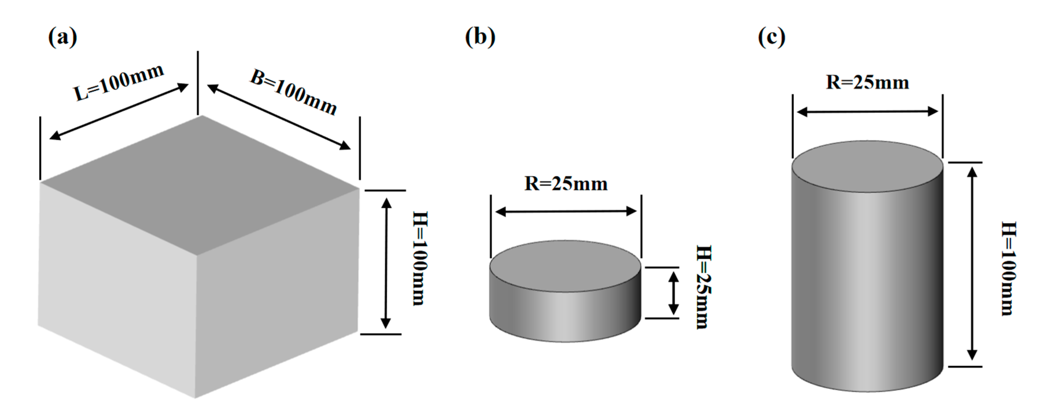
2.1. Specimen Preparation
2.2. Experimental Equipment and Setup
- (1)
- Loading equipment
- (2)
- AE monitoring system
3. AE Data Processing Methods
3.1. Inter-Event Time Function F(τ) Theory
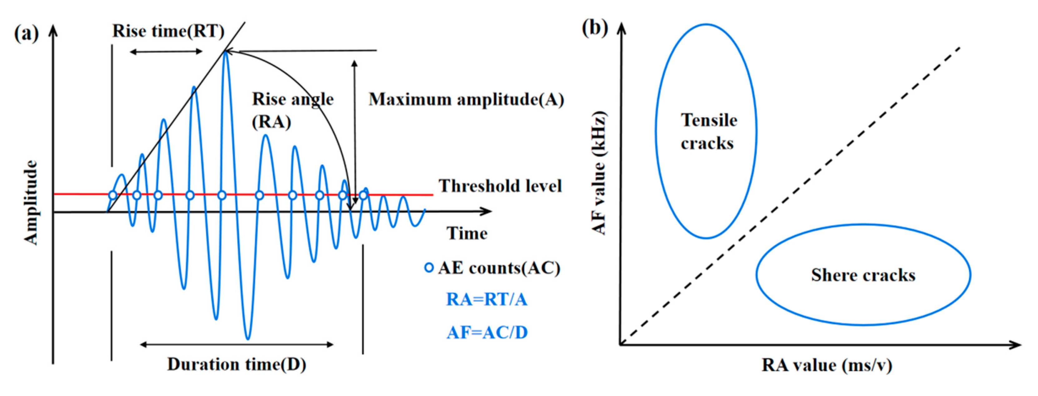
3.2. RA and AF Values Method
3.3. Kernel Density Estimation (KDE) Method
4. Experimental Results
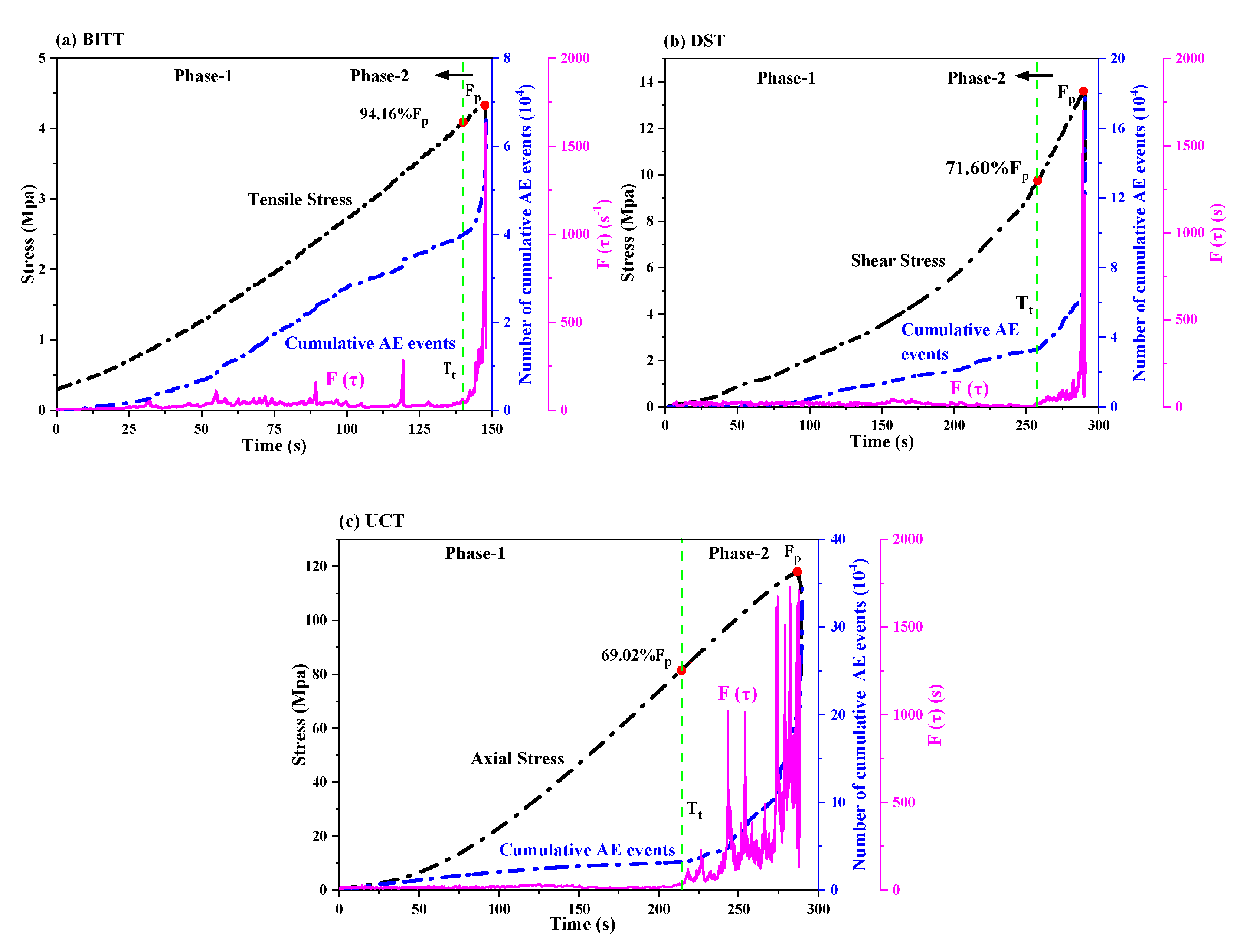
4.1. AE Event Rate Monitoring
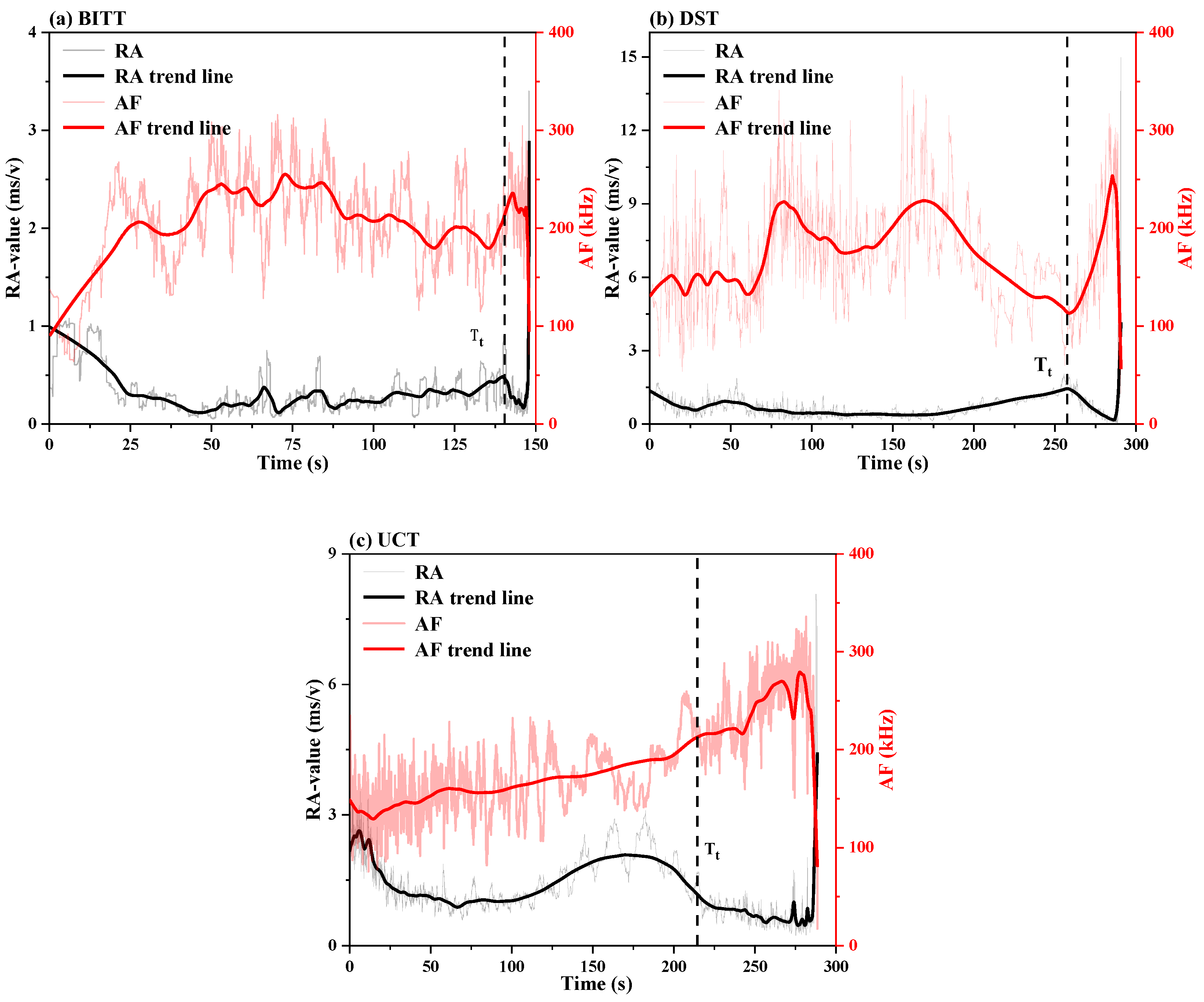
4.2. Evolution of RA and AF Values
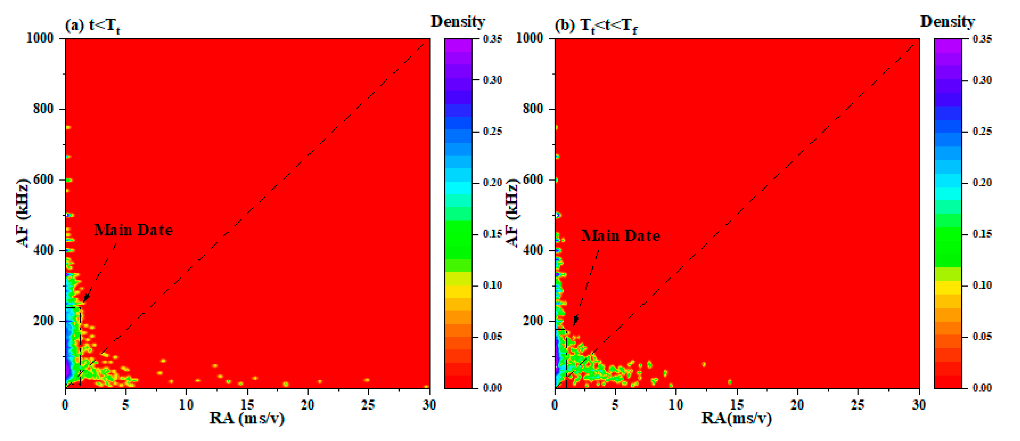
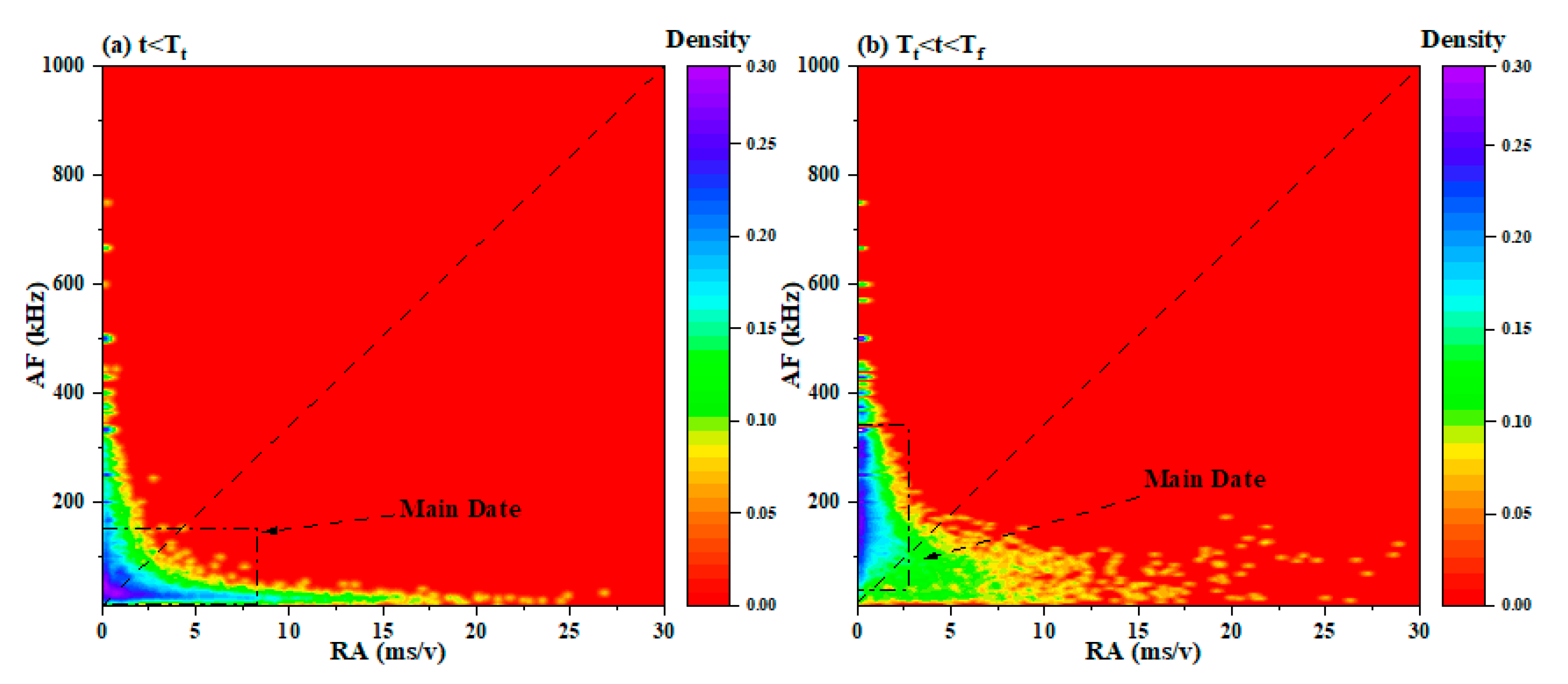
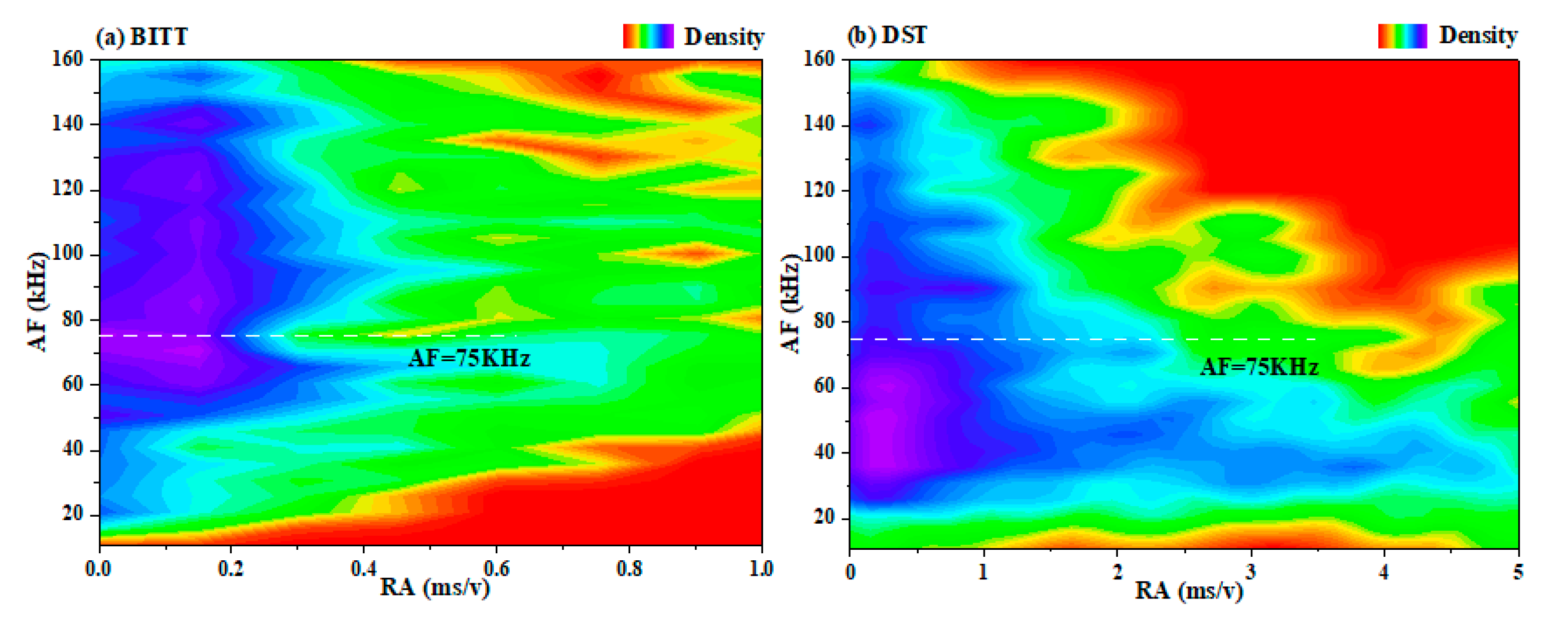
4.3. The Kernel Density Distribution of RA–AF Values
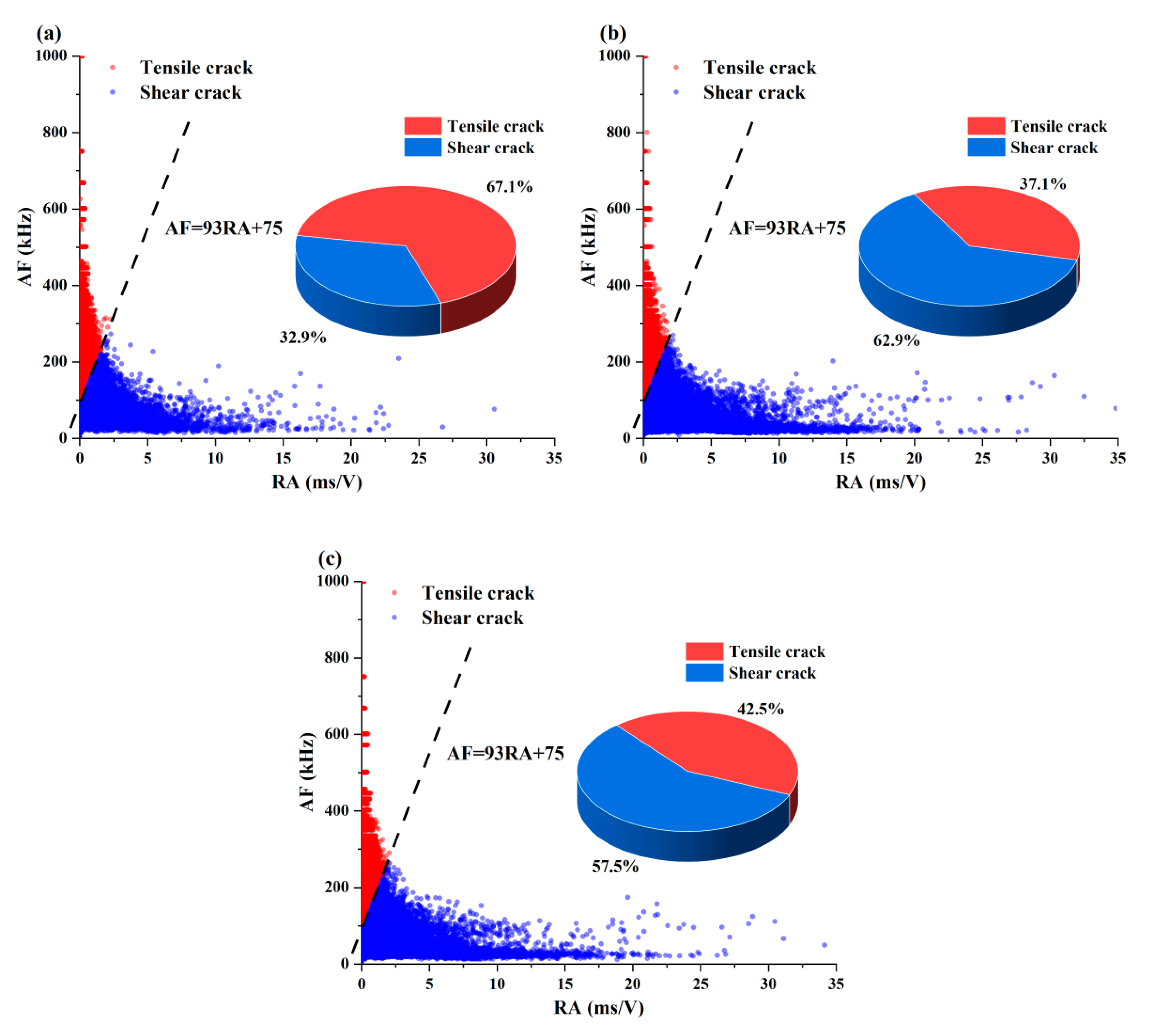
4.4. Classification of Tensile and Shear Cracks
4.5. Statistics of Tension and Shear Fracture, and Analysis of Failure Mechanism
5. Discussion
5.1. Evolution Characteristics of Tensile and Shear Sources in UCT
5.2. Failure Precursor Index of Rock Based on k Value
6. Conclusions
- (1)
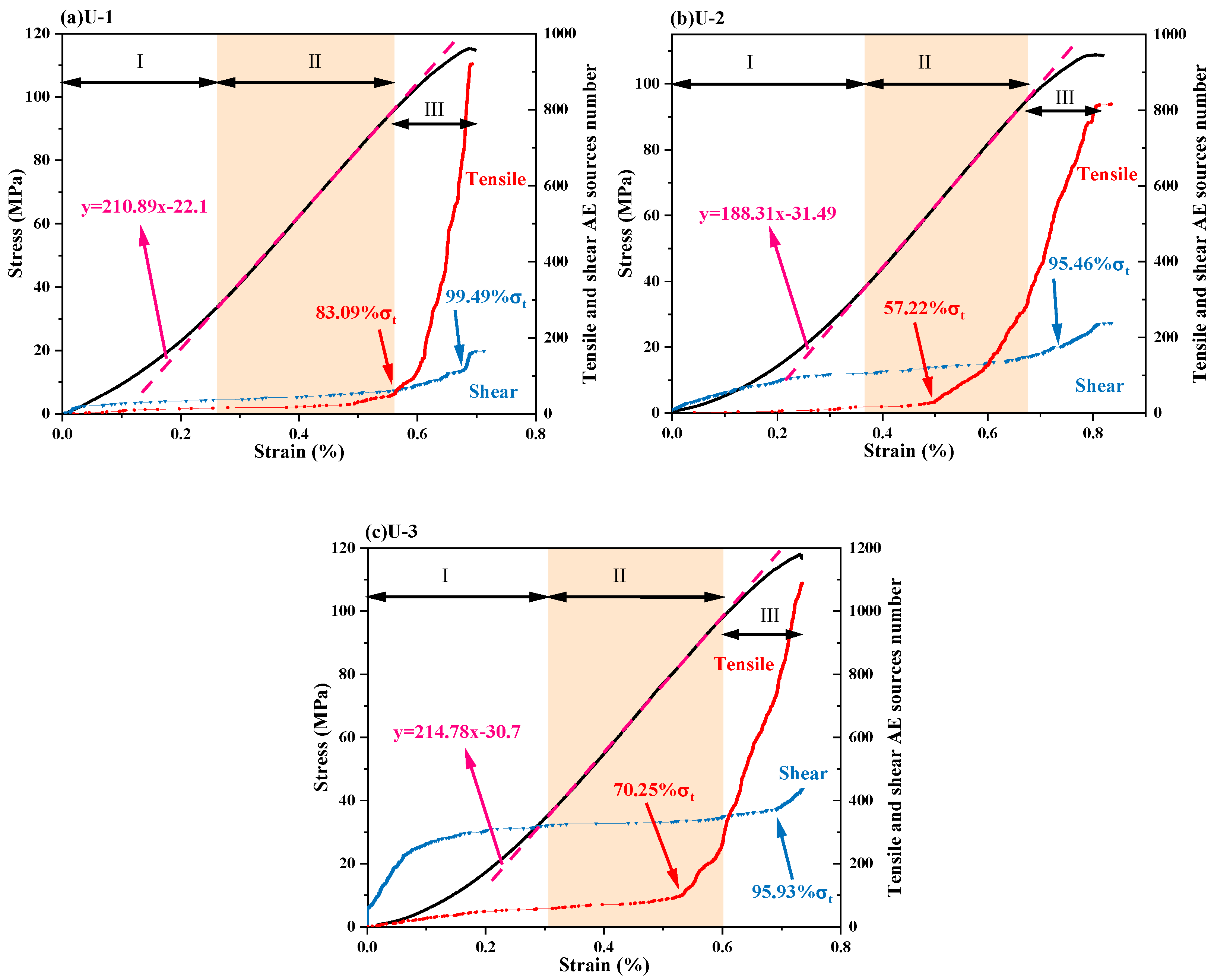
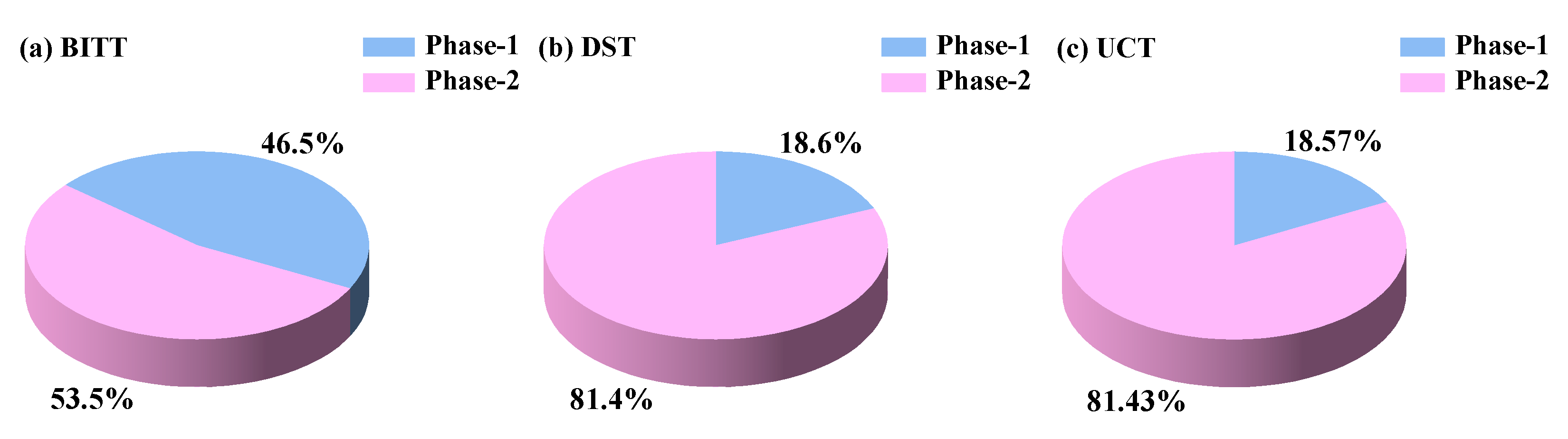
- AE event rate can reflect the transformation of rock samples from microcracks to macrocracks. The macrocrack generation phase in UCT was the longest, that in DST was the second longest, and that in BITT was the shortest;
- (2)
- The KDE method can effectively identify and visualize the high-density areas of RA and AF values. In the failure mode dominated by tensile fracture, the RA value was low and the AF value was high. On the contrary, in the failure mode dominated by shear fracture, the RA value was high and the AF value was low. When rock failure occurred, the RA and AF values both developed in opposite directions;
- (3)
- It was determined that the dividing line for classifying tensile and shear cracks in the RA and AF value data is AF = 93RA + 75. The reliability of the dividing line has been verified by analyzing the failure mode and fracture mechanism of the sample;
- (4)
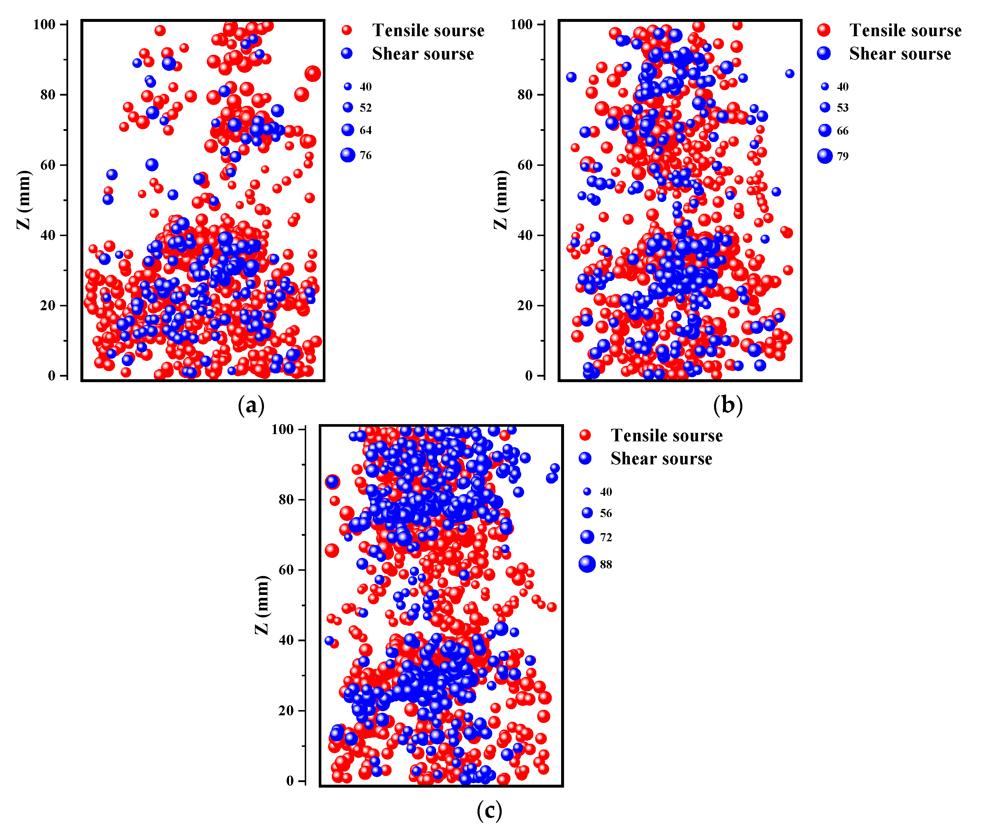
- Under uniaxial compression loading, the fracture source of red sandstone was mainly the shear source in the initial phase of loading, and the tensile source in the critical failure phase, and the number of the latter was far greater than that of the shear source;
- (5)
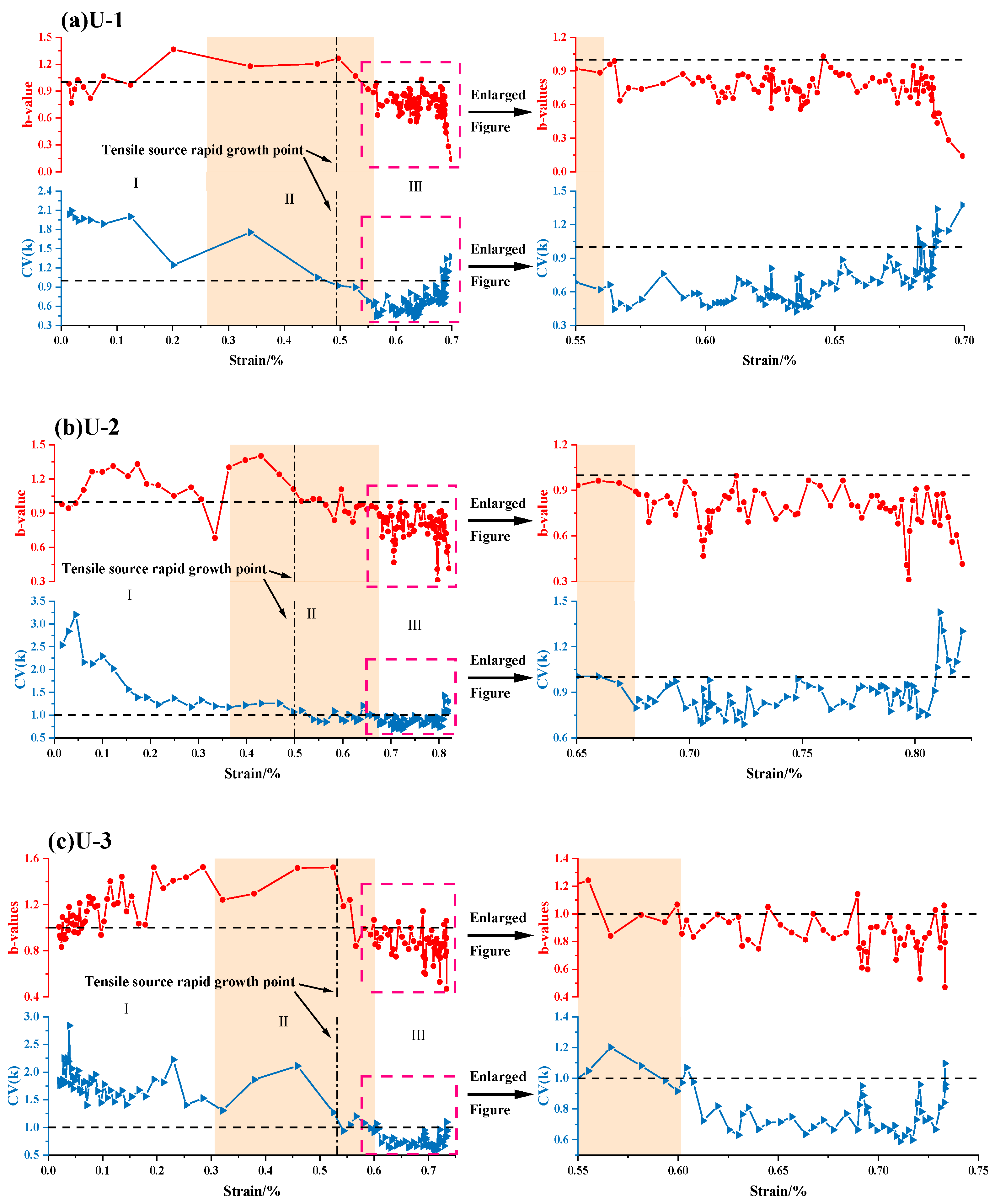
- K = AF/(93RA + 75) was proposed as an AE parameter index to reflect the internal fracture of the red sandstone specimen. Further, the corresponding reference judgment value CV (k) = 1 was proposed. It can be considered that the test sample entered the instability failure phase when CV (k) < 1.
Author Contributions
Funding
Institutional Review Board Statement
Informed Consent Statement
Data Availability Statement
Conflicts of Interest
Abbreviations
| AE | Acoustic emission |
| BITT | Brazilian indirect tensile test |
| DST | Direct shear test |
| UCT | Uniaxial compression test |
| KDE | Kernel density estimation |
| RA | RA = rise time/amplitude |
| AF | Average frequency |
| σs | Shear strength |
| σc | Uniaxial compressive strength |
| F(τ) | The inter-event time function/AE event rate |
| Tt | Time at the beginning of drastic increase in AE events |
| Ft | Load at the beginning of drastic increase in AE events |
| Fp | Peak load during the test |
| CV | The coefficient of variation |
References
- Bi, J.; Zhou, X.P.; Qian, Q.H. The 3D numerical simulation for the propagation process of multiple pre-existing flaws in Rock-Like materials subjected to biaxial compressive loads. Rock Mech. Rock Eng. 2016, 49, 1611–1627. [Google Scholar] [CrossRef]
- Zhao, Y.; Zhang, C.; Wang, Y.; Lin, H. Shear-related roughness classification and strength model of natural rock joint based on fuzzy comprehensive evaluation. Int. J. Rock Mech. Min. 2021, 137, 104550. [Google Scholar] [CrossRef]
- Zhao, Y.; Zhang, Y.; Yang, H.; Liu, Q.; Tian, G. Experimental study on relationship between fracture propagation and pumping parameters under constant pressure injection conditions. Fuel 2022, 307, 121789. [Google Scholar] [CrossRef]
- Tang, L.; Zhao, Y.; Liao, J.; Liu, Q. Creep experimental study of rocks containing weak interlayer under multilevel loading and unloading cycles. Front. Earth Sci. 2020, 480, 519461. [Google Scholar] [CrossRef]
- Zhao, Y.; He, P.; Zhang, Y.; Wang, C. A new criterion for a Toughness-Dominated hydraulic fracture crossing a natural frictional interface. Rock Mech. Rock Eng. 2019, 52, 2617–2629. [Google Scholar] [CrossRef]
- Zhao, Y.; Bi, J.; Wang, C.; Liu, P. Effect of unloading rate on the mechanical behavior and fracture characteristics of sandstones under complex triaxial stress conditions. Rock Mech. Rock Eng. 2021, 54, 4851–4866. [Google Scholar] [CrossRef]
- Zhao, Y.; Liu, Q.; Zhang, C.; Liao, J.; Lin, H.; Wang, Y. Coupled seepage-damage effect in fractured rock masses: Model development and a case study. Int. J. Rock Mech. Min. 2021, 144, 104822. [Google Scholar] [CrossRef]
- Zhao, Y.; Wang, Y.; Wang, W.; Tang, L.; Liu, Q.; Cheng, G. Modeling of rheological fracture behavior of rock cracks subjected to hydraulic pressure and far field stresses. Theor. Appl. Fract. Mech. 2019, 101, 59–66. [Google Scholar] [CrossRef]
- Zhao, Y.; Zhang, L.; Liao, J.; Wang, W.; Liu, Q.; Tang, L. Experimental study of fracture toughness and subcritical crack growth of three rocks under different environments. Int. J. Geomech. 2020, 20, 04020128. [Google Scholar] [CrossRef]
- Zhao, Y.; Wang, C.L.; Bi, J. Analysis of fractured rock permeability evolution under unloading conditions by the model of elastoplastic contact between rough surfaces. Rock Mech. Rock Eng. 2020, 53, 5795–5808. [Google Scholar] [CrossRef]
- Zhang, S.; Wu, S.; Chu, C.; Guo, P.; Zhang, G. Acoustic emission associated with Self-Sustaining failure in Low-Porosity sandstone under uniaxial compression. Rock Mech. Rock Eng. 2019, 52, 2067–2085. [Google Scholar] [CrossRef]
- Liang, Z.; Xue, R.; Xu, N.; Li, W. Characterizing rockbursts and analysis on frequency-spectrum evolutionary law of rockburst precursor based on microseismic monitoring. Tunn. Undergr. Space Tech. 2020, 105, 103564. [Google Scholar] [CrossRef]
- Aggelis, D.G. Classification of cracking mode in concrete by acoustic emission parameters. Mech. Res. Commun. 2011, 38, 153–157. [Google Scholar] [CrossRef]
- Aggelis, D.G.; Mpalaskas, A.C.; Matikas, T.E. Acoustic signature of different fracture modes in marble and cementitious materials under flexural load. Mech. Res. Commun. 2013, 47, 39–43. [Google Scholar] [CrossRef]
- Zhao, Y.; Ding, D.; Bi, J.; Wang, C.; Liu, P. Experimental study on mechanical properties of precast cracked concrete under different cooling methods. Constr. Build. Mater. 2021, 301, 124141. [Google Scholar] [CrossRef]
- Zhang, J.; Zhou, X. AE event rate characteristics of flawed granite: From damage stress to ultimate failure. Geophys. J. Int. 2020, 222, 795–814. [Google Scholar] [CrossRef]
- Jiang, R.; Dai, F.; Liu, Y.; Li, A.; Feng, P. Frequency characteristics of acoustic emissions induced by crack propagation in rock tensile fracture. Rock Mech. Rock Eng. 2021, 54, 2053–2065. [Google Scholar] [CrossRef]
- Zhou, X.; Zhang, J.; Qian, Q.; Niu, Y. Experimental investigation of progressive cracking processes in granite under uniaxial loading using digital imaging and AE techniques. J. Struct. Geol. 2019, 126, 129–145. [Google Scholar] [CrossRef]
- Fu, X.; Ban, Y.; Xie, Q.; Abdullah, R.A.; Duan, J. Time delay mechanism of the kaiser effect in sandstone under uniaxial compressive stress conditions. Rock Mech. Rock Eng. 2021, 54, 1091–1108. [Google Scholar] [CrossRef]
- Zhao, Y.; Zheng, K.; Wang, C.; Bi, J.; Zhang, H. Investigation on model-I fracture toughness of sandstone with the structure of typical bedding inclination angles subjected to three-point bending. Theor. Appl. Fract. Mec. 2022, 119, 103327. [Google Scholar] [CrossRef]
- Yang, H.; Lin, H.; Chen, Y.; Wang, Y.; Zhao, Y.; Yong, W.; Gao, F. Influence of wing crack propagation on the failure process and strength of fractured specimens. Bull. Eng. Geol. Environ. 2022, 81, 71. [Google Scholar] [CrossRef]
- Liao, J.; Zhao, Y.; Tang, L.; Liu, Q.; Sarmadivaleh, M. Experimental Studies on Cracking and Local Strain Behaviors of Rock-Like Materials with a Single Hole before and after Reinforcement under Biaxial Compression. Geofluids 2021, 8812006. [Google Scholar] [CrossRef]
- Zhao, Y.; Wang, Y.; Tang, L. The compressive-shear fracture strength of rock containing water based on Druker-Prager failure criterion. Arab. J. Geosci. 2019, 12, 452. [Google Scholar] [CrossRef]
- Lacidogna, G.; Piana, G.; Accornero, F.; Carpinteri, A. Multi-technique damage monitoring of concrete beams: Acoustic Emission, Digital Image Correlation, Dynamic Identification. Constr. Build. Mater. 2020, 242, 118114. [Google Scholar] [CrossRef]
- Zhang, Z.; Deng, J. A new method for determining the crack classification criterion in acoustic emission parameter analysis. Int. J. Rock Mech. Min. 2020, 130, 104323. [Google Scholar] [CrossRef]
- Du, K.; Li, X.; Tao, M.; Wang, S. Experimental study on acoustic emission (AE) characteristics and crack classification during rock fracture in several basic lab tests. Int. J. Rock Mech. Min. 2020, 133, 104411. [Google Scholar] [CrossRef]
- Zhao, Y.; Zhang, L.; Wang, W.; Tang, J.; Lin, H.; Wan, W. Transient pulse test and morphological analysis of single rock fractures. Int. J. Rock Mech. Min. 2017, 91, 139–154. [Google Scholar] [CrossRef]
- Zhao, Y.; Liu, Q.; Liao, J.; Wang, Y.; Tang, L. Theoretical and numerical models of rock wing crack subjected to hydraulic pressure and far-field stresses. Arab. J. Geosci. 2020, 13, 926. [Google Scholar] [CrossRef]
- Chai, M.; Hou, X.; Zhang, Z.; Duan, Q. Identification and prediction of fatigue crack growth under different stress ratios using acoustic emission data. Int. J. Fatigue 2022, 160, 106860. [Google Scholar] [CrossRef]
- Zhang, F.; Yang, Y.; Fennis, S.A.A.M.; Hendriks, M.A.N. Developing a new acoustic emission source classification criterion for concrete structures based on signal parameters. Constr. Build. Mater. 2022, 318, 126163. [Google Scholar] [CrossRef]
- Dong, L.; Tong, X.; Ma, J. Quantitative investigation of tomographic effects in abnormal regions of complex structures. Engineering 2021, 7, 1011–1022. [Google Scholar] [CrossRef]
- Gan, Y.; Wu, S.; Ren, Y.; Zhang, G. Evaluation indexes of granite splitting failure based on RA and AF of AE parameters. Rock Soil Mech. 2020, 41, 2324–2332. [Google Scholar]
- Zhao, Y.; Zhang, L.; Wang, W.; Pu, C.; Wan, W.; Tang, J. Cracking and stress–strain behavior of Rock-Like material containing two flaws under uniaxial compression. Rock Mech. Rock Eng. 2016, 49, 2665–2687. [Google Scholar] [CrossRef]
- Tang, Y.; Lin, H.; Wang, Y.; Zhao, Y. Rock slope stability analysis considering the effect of locked section. Bull. Eng. Geol. Environ. 2021, 80, 7241–7251. [Google Scholar] [CrossRef]
- Ohno, K.; Ohtsu, M. Crack classification in concrete based on acoustic emission. Constr. Build. Mater. 2010, 24, 2339–2346. [Google Scholar] [CrossRef]
- JCMS-III B5706; Monitoring Method for Active Cracks in Concrete by Acoustic Emission. Federation of Construction Materials Industries: Tokyo, Japan, 2003.
- Ohtsu, M. Rilem Technical Committee (Ohtsu M. Recommendation of RILEM TC 212-ACD: Acoustic emission and related NDE techniques for crack detection and damage evaluation in concrete. Mater. Struct. 2010, 43, 1187–1189. [Google Scholar]
- Zhao, Y.; Liao, J.; Wang, Y.; Liu, Q.; Lin, H.; Chang, L. Crack coalescence patterns and local strain behaviors near flaw tip for rock-like material containing two flaws subjected to biaxial compression. Arab. J. Geosci. 2020, 13, 1251. [Google Scholar] [CrossRef]
- Wang, H.; Liu, D.; Cui, Z.; Cheng, C.; Jian, Z. Investigation of the fracture modes of red sandstone using XFEM and acoustic emissions. Theor. Appl. Fract. Mech. 2016, 85, 283–293. [Google Scholar] [CrossRef]
- Lotidis, M.A.; Nomikos, P.P. Acoustic emission location analysis and microcracks’ nature determination of uniaxially compressed calcitic marble hollow plates. Geomech. Geophys. Geo-Energy Geo-Resour. 2021, 7, 38. [Google Scholar] [CrossRef]
- Li, D.; Du, F. Monitoring and evaluating the failure behavior of ice structure using the acoustic emission technique. Cold Reg. Sci. Technol. 2016, 129, 51–59. [Google Scholar] [CrossRef]
- Han, Q.; Yang, G.; Xu, J.; Fu, Z.; Lacidogna, G.; Carpinteri, A. Acoustic emission data analyses based on crumb rubber concrete beam bending tests. Eng. Fract. Mech. 2019, 210, 189–202. [Google Scholar] [CrossRef]
- Triantis, D. Acoustic emission monitoring of marble specimens under uniaxial compression. Precursor phenomena in the near-failure phase. Proced. Struct. Integr. 2018, 10, 11–17. [Google Scholar] [CrossRef]
- Xie, Q.; Li, S.; Liu, X.; Gong, F.; Li, X. Effect of loading rate on fracture behaviors of shale under mode I loading. J. Cent. South Univ. 2020, 27, 3118–3132. [Google Scholar] [CrossRef]
- Wang, Y.; Peng, K.; Shang, X.; Li, L.; Liu, Z.; Wu, Y.; Long, K. Experimental and numerical simulation study of crack coalescence modes and microcrack propagation law of fissured sandstone under uniaxial compression. Theor. Appl. Fract. Mech. 2021, 115, 103060. [Google Scholar] [CrossRef]
- Liu, X.; Liu, Z.; Li, X.; Gong, F.; Du, K. Experimental study on the effect of strain rate on rock acoustic emission characteristics. Int. J. Rock Mech. Min. 2020, 133, 104420. [Google Scholar] [CrossRef]
- Zhang, H.; Wang, Z.; Song, Z.; Zhang, Y.; Wang, T.; Zhao, W. Acoustic emission characteristics of different brittle rocks and its application in brittleness evaluation. Geomech. Geophys. Geo-Energy Geo-Resour. 2021, 7, 48. [Google Scholar] [CrossRef]
- Meng, Y.; Jing, H.; Liu, X.; Yin, Q.; Wei, X. Experimental and numerical investigation on the effects of bedding plane properties on the mechanical and acoustic emission characteristics of sandy mudstone. Eng. Fract. Mech. 2021, 245, 107582. [Google Scholar] [CrossRef]
- Ge, Z.; Sun, Q. Acoustic emission characteristics of gabbro after microwave heating. Int. J. Rock Mech. Min. 2021, 138, 104616. [Google Scholar] [CrossRef]
- Chang, X.; Zhang, X.; Dang, F.; Zhang, B.; Chang, F. Failure behavior of sandstone specimens containing a single flaw under true triaxial compression. Rock Mech. Rock Eng. 2022. [Google Scholar] [CrossRef]
- Muñoz-Ibáñez, A.; Delgado-Martín, J.; Herbón-Penabad, M.; Alvarellos-Iglesias, J. Acoustic emission monitoring of mode I fracture toughness tests on sandstone rocks. J. Petrol. Sci. Eng. 2021, 205, 108906. [Google Scholar] [CrossRef]
- Li, L.R.; Deng, J.H.; Zheng, L.; Liu, J.F. Dominant frequency characteristics of acoustic emissions in white marble during direct tensile tests. Rock Mech. Rock Eng. 2017, 50, 1337–1346. [Google Scholar] [CrossRef]
- Niu, Y.; Zhou, X.; Berto, F. Evaluation of fracture mode classification in flawed red sandstone under uniaxial compression. Theor. Appl. Fract. Mec. 2020, 107, 102528. [Google Scholar] [CrossRef]
- Wang, Y.; Zhang, B.; Gao, S.H.; Li, C.H. Investigation on the effect of freeze-thaw on fracture mode classification in marble subjected to multi-level cyclic loads. Theor. Appl. Fract. Mech. 2021, 111, 102847. [Google Scholar] [CrossRef]
- Wang, Y.; Meng, H.; Long, D. Experimental investigation of fatigue crack propagation in interbedded marble under multilevel cyclic uniaxial compressive loads. Fatigue Fract. Eng. Mater. Struct. 2021, 44, 933–951. [Google Scholar] [CrossRef]
- Yao, Q.; Chen, T.; Tang, C.; Sedighi, M.; Wang, S.; Huang, Q. Influence of moisture on crack propagation in coal and its failure modes. Eng. Geol. 2019, 258, 105156. [Google Scholar] [CrossRef]
- Xiangqian, F.; Shengtao, L.; Xudong, C.; Saisai, L.; Yuzhu, G. Fracture behaviour analysis of the full-graded concrete based on digital image correlation and acoustic emission technique. Fatigue Fract. Eng. Mater. Struct. 2020, 43, 1274–1289. [Google Scholar] [CrossRef]
- Das, A.K.; Suthar, D.; Leung, C.K.Y. Machine learning based crack mode classification from unlabeled acoustic emission waveform features. Cem. Concr. Res. 2019, 121, 42–57. [Google Scholar] [CrossRef]
- Dong, L.; Chen, Y.; Sun, D.; Zhang, Y. Implications for rock instability precursors and principal stress direction from rock acoustic experiments. Int. J. Min. Sci. Technol. 2021, 31, 789–798. [Google Scholar] [CrossRef]
- Prem, P.R.; Murthy, A.R. Acoustic emission monitoring of reinforced concrete beams subjected to four-point-bending. Appl. Acoust. 2017, 117, 28–38. [Google Scholar] [CrossRef]
- Sagar, R.V.; Srivastava, J.; Singh, R.K. A probabilistic analysis of acoustic emission events and associated energy release during formation of shear and tensile cracks in cementitious materials under uniaxial compression. J. Build. Eng. 2018, 20, 647–662. [Google Scholar] [CrossRef]
- Triantis, D.; Kourkoulis, S.K. An alternative approach for representing the data provided by the acoustic emission technique. Rock Mech. Rock Eng. 2018, 51, 2433–2438. [Google Scholar] [CrossRef]
- Rippengill, S.; Worden, K.; Holford, K.M.; Pullin, R. Automatic classification of acoustic emission patterns. Strain 2003, 39, 31–41. [Google Scholar] [CrossRef]
- Wawersik, W.R. Detailed Analysis of Rock Failure in Laboratory Compression Tests; University of Minnesota: Minneapolis, MN, USA, 1968. [Google Scholar]
- Hoek, E. Brittle fracture of rock. Rock Mech. Eng. Pract. 1968, 130, 9–124. [Google Scholar]
- Jaeger, J.C. “Brittle Fracture of Rocks.” The 8th US Symposium on Rock Mechanics (USRMS); OnePetro: Richardson, TX, USA, 1966. [Google Scholar]
- Li, M.; Qu, Y.; Qin, S.; Yan, X.; Sun, Q.; Ma, P. Criteria of swelling potential and analysis on failure mechanism for mud rock. J. Eng. Geol. 2009, 17, 633–637. [Google Scholar]
- Chen, J.; Li, S. Fracture failure mechanism of rock. Adv. Earth Sci. 2004, 19, 275–278. [Google Scholar]
- Zhao, Y.; Wang, C.; Ning, L.; Zhao, H.; Bi, J. Pore and fracture development in coal under stress conditions based on nuclear magnetic resonance and fractal theory. Fuel 2022, 309, 122112. [Google Scholar] [CrossRef]
- Sagasta, F.; Zitto, M.E.; Piotrkowski, R.; Benavent-Climent, A.; Suarez, E.; Gallego, A. Acoustic emission energy b-value for local damage evaluation in reinforced concrete structures subjected to seismic loadings. Mech. Syst. Signal Process. 2018, 102, 262–277. [Google Scholar] [CrossRef]
- Guo, P.; Wu, S.; Zhang, G.; Chu, C. Effects of thermally-induced cracks on acoustic emission characteristics of granite under tensile conditions. Int. J. Rock Mech. Min. 2021, 144, 104820. [Google Scholar] [CrossRef]


| Number | Type of Test | Loading Rate (mm/min) | σt/σs/σc (MPa) |
|---|---|---|---|
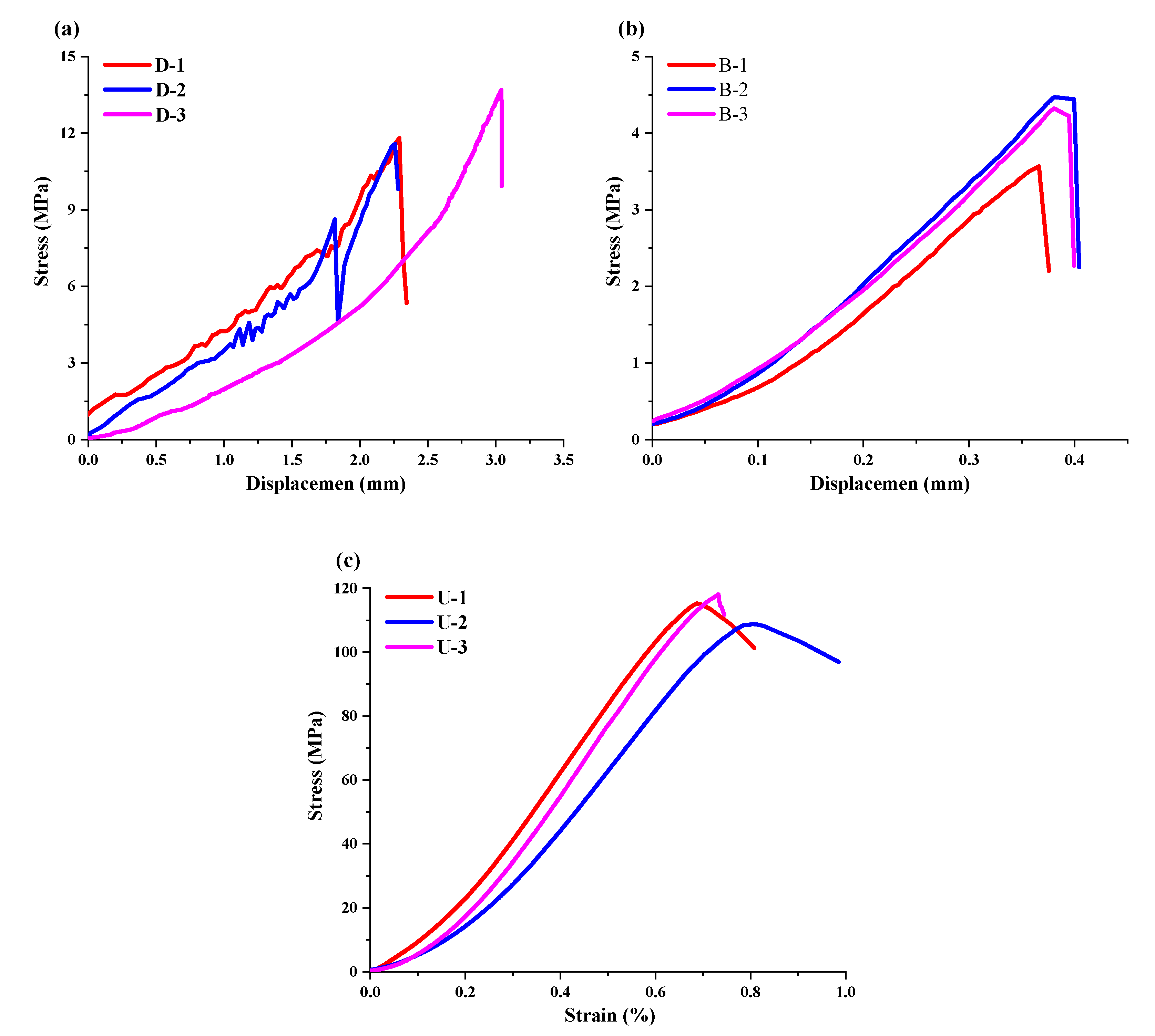
| B-1 | BITT | 0.05 | 7.06 |
| B-2 | 8.50 | ||
| B-3 | 8.80 | ||
| D-1 | DST | 0.1 | 12.48 |
| D-2 | 11.79 | ||
| D-3 | 13.68 | ||
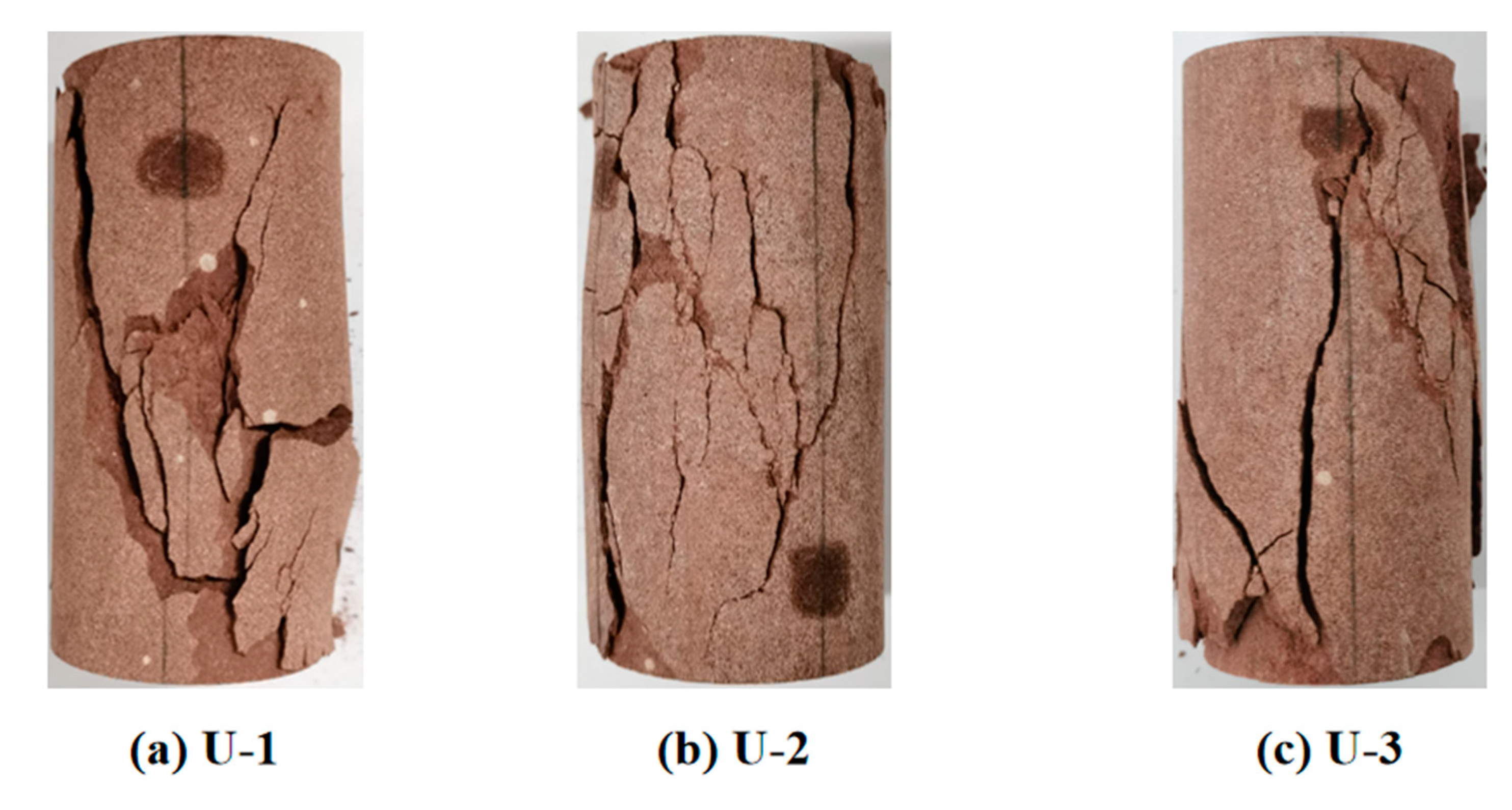
| U-1 | UCT | 0.1 | 115.27 |
| U-2 | 108.79 | ||
| U-3 | 118.10 |
Publisher’s Note: MDPI stays neutral with regard to jurisdictional claims in published maps and institutional affiliations. |
© 2022 by the authors. Licensee MDPI, Basel, Switzerland. This article is an open access article distributed under the terms and conditions of the Creative Commons Attribution (CC BY) license (https://creativecommons.org/licenses/by/4.0/).
Share and Cite
Li, J.; Lian, S.; Huang, Y.; Wang, C. Study on Crack Classification Criterion and Failure Evaluation Index of Red Sandstone Based on Acoustic Emission Parameter Analysis. Sustainability 2022, 14, 5143. https://doi.org/10.3390/su14095143
Li J, Lian S, Huang Y, Wang C. Study on Crack Classification Criterion and Failure Evaluation Index of Red Sandstone Based on Acoustic Emission Parameter Analysis. Sustainability. 2022; 14(9):5143. https://doi.org/10.3390/su14095143
Chicago/Turabian StyleLi, Jiashen, Shuailong Lian, Yansen Huang, and Chaolin Wang. 2022. "Study on Crack Classification Criterion and Failure Evaluation Index of Red Sandstone Based on Acoustic Emission Parameter Analysis" Sustainability 14, no. 9: 5143. https://doi.org/10.3390/su14095143
APA StyleLi, J., Lian, S., Huang, Y., & Wang, C. (2022). Study on Crack Classification Criterion and Failure Evaluation Index of Red Sandstone Based on Acoustic Emission Parameter Analysis. Sustainability, 14(9), 5143. https://doi.org/10.3390/su14095143