A Joint Scheduling Strategy for Wind and Solar Photovoltaic Systems to Grasp Imbalance Cost in Competitive Market

Abstract

The integration of renewable energy sources with active thermal power plants contributes to the green environment all over the globe. To achieve maximum reliability and sustainability of the renewable-thermal hybrid system, plentiful constraints need to be considered for minimizing the situation, which creates due to the unpredictable nature of renewable energy. In wind integrated deregulated system, wind farms need to submit the power generation scenario for future days to Independent System Operator (ISO) before the date of operation. Based on their submitted bid, ISO scheduled the power generation from different generating stations, including thermal and renewable. Due to the uncertain nature of the wind flow, there is always a chance of not fulfilling the scheduling amount of power from the wind farm. This violation in the market can impose an economic burden (i.e., imbalance cost) on the generating companies. The solar photovoltaic cell can be used to decrease the adverse economic effects of unpredicted wind saturation in the deregulated system. This paper presents consistent, competent, and effective operating schemes for the hybrid operation of solar PV and wind farms to maximize the economic profit by minimizing the imbalance cost, which occurs due to the mismatch between the actual and predicted wind speed. Modified IEEE 14-bus and modified IEEE 30-bus test systems have been used to check the usefulness of the proposed approach. Three optimization techniques (i.e., Sequential Quadratic Programming (SQP), Smart Flower Optimization Algorithm (SFOA), Honey Badger Algorithm (HBA)) have been used in this work for the comparative study. Bus Loading Factor (BLF) has been proposed here to identify the most sensitive bus in the system, used to place wind farms. The SFOA and HBA optimization technique has been used first time in this type of economic assessment problem, which is the novelty of this paper. The Bus Loading Factor (BLF) has been introduced here to identify the most sensitive bus in the system. After implementing the work, it has been seen that the operation of the solar PV system has reduced the adverse effect of imbalance cost on the renewable integrated deregulated power system.

1. Introduction

In recent years, the energy requirement has been augmented at a very high rate owing to the modernization and advancement of electrical appliances. Simultaneously due to the economic, social, political, and environmental barriers, it is difficult to construct new power plants [1]. The quantity of available coal along with the fossil fuels has decreased day by day, which creates a lot of pressure on the power plant personnel as well as on the Governments. This situation forces the Government and Generation companies (GENCOS) to contemplate incorporating renewable energy sources with the existing power plants. Wind and solar energy are the most used sources among all the renewable energy sources due to their easy availability, no running cost phenomenon. The uncertain nature of wind and solar energy generation as well as their performance detoriation in time [2], bound the GENCOS to use energy storage devices as backup sources. Pumped hydro storage (PHS), compressed air energy storage (CAES), and batteries are mostly used energy storage devices. Like several developed and developing countries, the Government of India (GoI) is also targeting to make India a renewable dominating country. GoI has set a target to generate 175 GW of power from renewable energy sources, among which 100 GW from solar, 60 GW from wind, and the remaining from other renewable sources [3].

Nowadays, the power industry is transforming from a regulated to deregulated concept. In the regulated power market, there was very limited transparency in economic aspects between GENCOS and customers. This environment may benefit the GENCOS, but customers are the sufferers of this concept. So, a new market environment named deregulation has been introduced to enhance customer benefits. Deregulated power market has created lots of competition among their market players i.e., GENCOS, Transmission Companies (TRANSCOS), Distribution Companies (DISCOS), and retailers. Due to the increased transparency and competition, customers benefit from this system. ISO plays an important role in this type of scenario by participating as the controller of the electricity market. At first, ISO collects the bid from the GENCOS as well as from the DISCOS. After performing the optimization, ISO fixed the market-clearing price (MCP) and Market Clearing Volume (MCV), at which point the generators and customers both got the benefit.

The renewable power integration with the existing thermal power plant in the deregulated power system is very complex, but the customer got the welfare. In the recent past, several researchers have done some work in this field. Xiangsheng et al. [4] proposed a framework in the electricity market for the summation of large-scale prosumers. Mohammad Rasol Jannisar et al. [5] focused on the battery storage performance, sizing, charge/discharge, and optimal placement, which are based upon cost functions, environmental emission, and transmission usage fee of the battery storage system.

Different comprehensive studies on participation in the optimal market, encouraging policies, optimal bidding approach, progress in the electricity market, and cooperative contribution of renewable energy systems in the electricity markets have been projected in [6]. Optimal bidding proposal for a day-ahead electricity market due to the problem of combined operation between wind and photovoltaic power systems with the energy storage device is extensively studied in [7]. Yang Zhang et al. [8] has proposed a strategy for rule-based operation and simultaneously improve the capacity of the battery. In [9], the author investigates that with a capacitive energy storage unit, a sine cosine algorithm develops a proportional-integral controller that provides improved dynamic reaction in all the states of the day-ahead electricity market under different situations. Arezoo Hasankhani et al. [10] project a probabilistic algorithm for energy management to direct the involvement of smart microgrids in the electricity market. In [11], the author has focused on the optimization methods of operation and scheduling of pump storage and wind plant under the day-ahead power market.

Work in [12] presents a stochastic approach in which the authors combine the ideal solar performance with a survey of weather measurements and estimate the next day’s solar generation, which determines a conditional probability distribution. Chenxi Zhang et al. [13] have proposed a model for trading oriented battery energy storage for a distribution system that is constructed with multi-objective and mutual-iteration two-stage optimization. A case study at Ado Ekiti, South-West Nigeria, on the combination of Diesel/PV/Biogas backup for unstable grid electricity has been discussed in [14]. Sahoo et al. [15] present a bidding methodology for the impact assessment of energy storage devices and distributed resources in deregulated micro-grid. In [16], a short-term scheduling problem has been solved by the authors by considering different models of deregulation. An optimal energy management strategy for micro-grid has been discussed in [17] in competitive power systems. Lakiotis et al. [18] depict an assessment methodology of the functioning worth of energy storage system by mid-term simulation method.

Recently, nature-inspired algorithms have become very popular for addressing power systems issues. A special use case seems to be addressing novel issues that arise due to the penetration of renewable energy technologies [19,20,21]. There are some works where economic studies have also been performed with these optimization approaches. In [22], authors have investigated the use of hybrid firefly particle swarm optimization (HFPSO) for a day-ahead demand-side management system that is geared towards systems with high renewable energy penetration. The management system is programmed to minimize fuel costs as well as carbon emissions. However, it does not consider a cost-competitive market model. In [23], the salp swarm technique is utilized for an isolated hybrid microgrid control. The objective is optimal frequency stabilization with price-based demand response. Thermastatically controllable loads are considered in this scheme for achieving frequency stability in the isolated microgrid. Although the proposed scheme is focused on price, it deals with non-critical loads and not generators. Habib et al. [24] present a methodology to minimize the energy cost of a renewable integrated vehicle-to-grid system using the Artificial Bee Colony (ABC) algorithm. An optimal demand-side response strategy has been depicted in [25] for a multiple microgrid system using an improved co-evolution algorithm. Paper [26] presents the strategy for mitigating the imbalance using variable PV ancillary services.

From the literature studies, it can seem that some economic assessment work has been completed by several researchers in the past, but there are some questions still there which have been done in this work: (a) What will be the impact of energy bidding in the wind integrated deregulated power system? (b) What will be the effect of imbalance cost in a day-ahead electrical system? (c) How do optimal operations of solar PV provide a better economy in a renewable integrated system with considering imbalance cost? (d) How do different optimization approaches provide superior cost-effective payback for a hybrid electrical system?

The main contributions of this work are as follows:

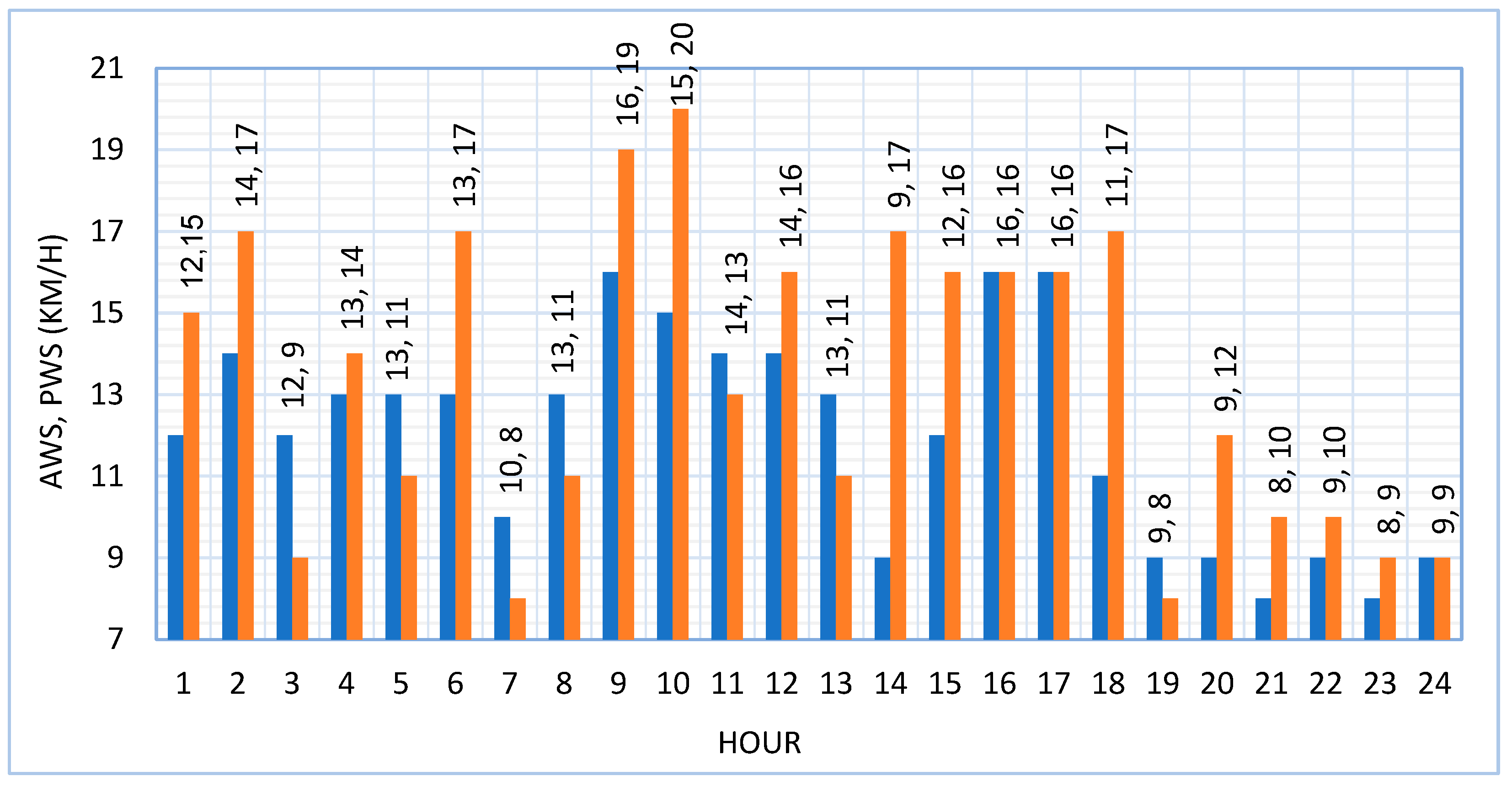
• The importance of imbalance cost has been studied, which is arisen due to the disparity between actual wind speed (AWS) and predicted wind speed (PWS). When actual wind power (AWP) is more than the predicted wind power (PWP), then ISO rewards the wind farm for their surplus power supply, and on the other hand, ISO imposes a penalty if PWP is more than AWP.
• The adverse effect of imbalance cost directly disturbs the economic advancement of the market players. This work exhibits the effect of solar PV in the system economy of a hybrid wind farm-solar PV deregulated power system.
• The investigation is carried out by several optimization techniques (i.e., SQP, SFOA, HBA). The SFOA and HBA have been used first time in this type of economic problem, which is the novelty of this paper.

In this paper, Section 1 introduces the overview of the problem yet to be solved. Section 2 discusses the system modeling, including solar PV, wind farm, and BLF. A brief description of the used optimization techniques is given in Section 3. The detailed problem formulation with its constraints is mentioned in Section 4. Section 5 shows the implementation and outcome of the proposed approach. Lastly, Section 6 indicates the conclusion drawn from the exponent.

2. System Modeling

A hybrid system may contain different renewable energy sources like solar PV, wind turbines as well as non-renewable generators like storage devices, micro-turbine, etc. A hybrid system might be a combination of a few or all of them.

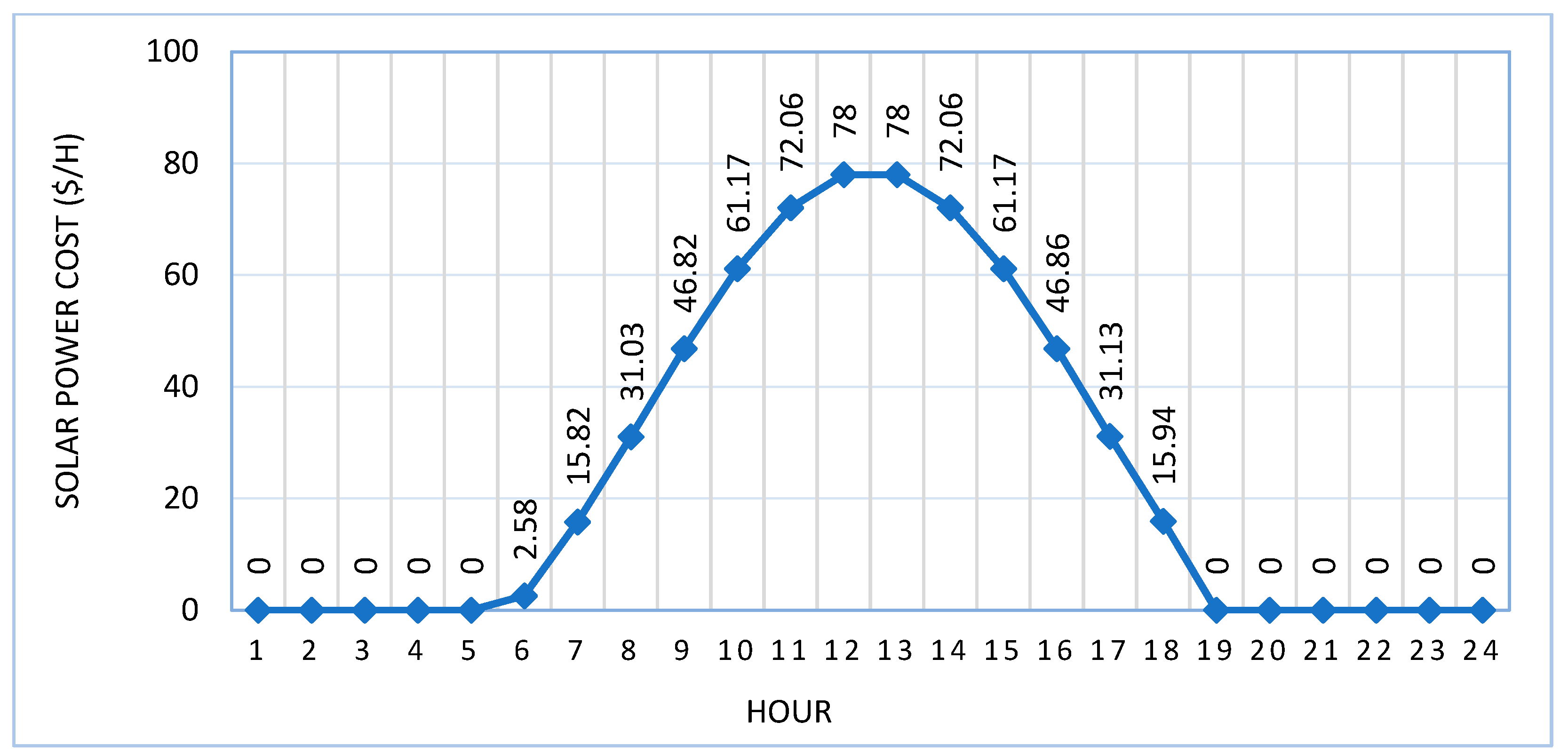
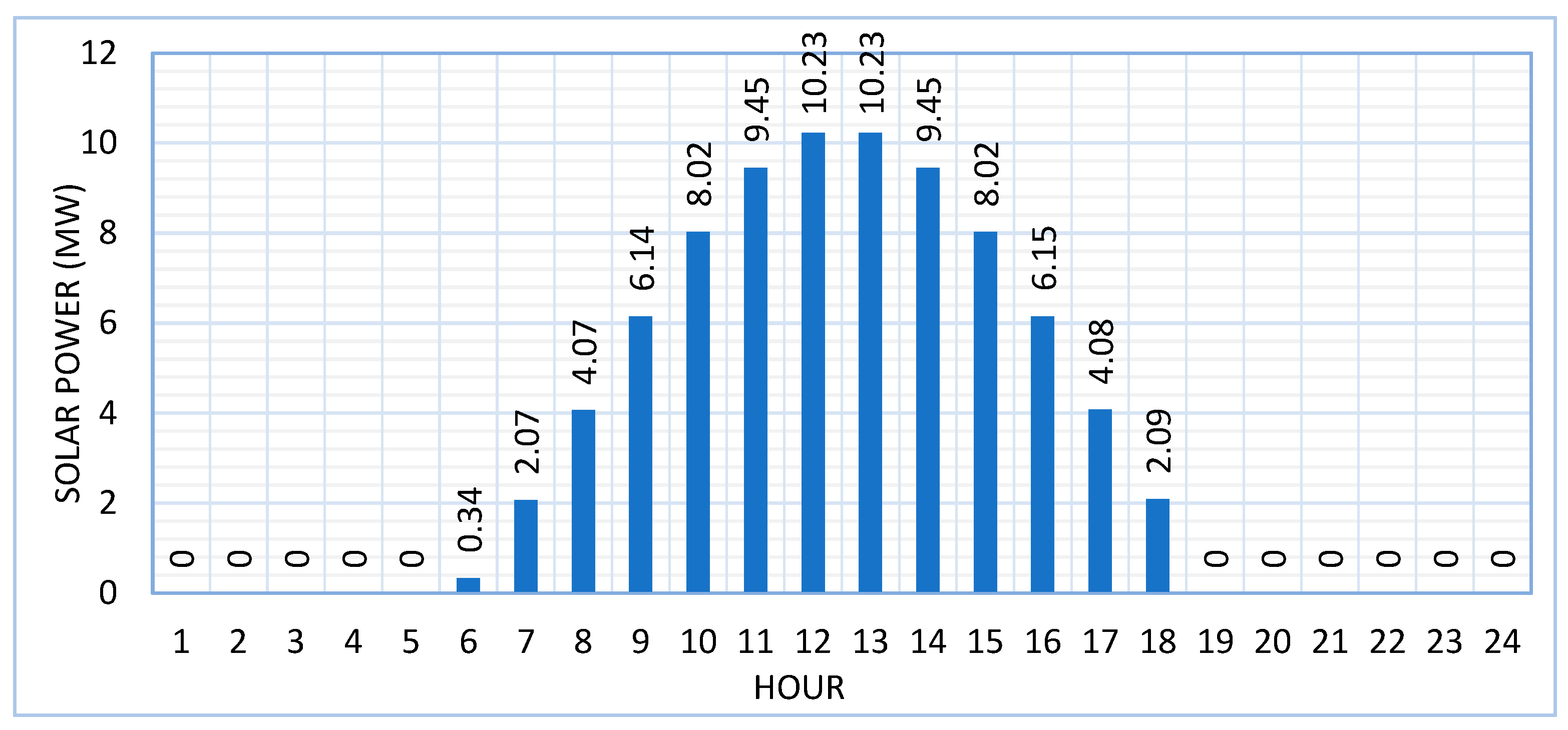
2.1. Solar PV System

The output of solar PV arrays depends on the ambient temperature and solar irradiance. Output power (P_ph) of this model is calculated as [27]

$$P_{\mathrm{p}\mathrm{h}}={\mathsf{\eta }}_{\mathrm{p}\mathrm{h}\mathrm{g}}{\mathrm{A}}_{\mathrm{p}\mathrm{h}\mathrm{g}}{\mathrm{G}}_{\mathrm{t}}$$

(1)

where η_phg is the efficiency of generation in PV array, A_phg is generator area in PV array, and G_t is solar irradiation in slanted segment level (W/m²). Further η_phg is

$${\mathsf{\eta }}_{\mathrm{p}\mathrm{h}\mathrm{g}}={\mathsf{\eta }}_{\mathrm{r}}{\mathsf{\eta }}_{\mathrm{p}\mathrm{c}}\left[1-\mathsf{\beta }\left({\mathrm{T}}_{\mathrm{c}}-{\mathrm{T}}_{\mathrm{c},\mathrm{r}\mathrm{e}\mathrm{f}}\right)\right]$$

(2)

when Maximum Power Point Tracking (MPPT) is used, then power conditioning efficiency (η_pc) is equal to one. η_r is the efficiency of the reference module. The temperature coefficient is denoted by β, the range is between (0.004–0.006) per °C). Reference cell temperature is denoted by T_c,ref in °C, and T_c,ref can be obtained by the following relation:

$${\mathrm{T}}_{\mathrm{c}}={\mathrm{T}}_{\mathrm{a}\mathrm{t}}+\frac{\left({\mathrm{T}}_{\mathrm{N}\mathrm{O}\mathrm{C}}-20\right){\mathrm{G}}_{\mathrm{t}}}{800}$$

(3)

Here T_at is the ambient temperature (°C) and T_NOC is the nominal operating cell temperature (°C). The total solar radiation in the solar cell can be estimated because of normal and diffuse solar radiation as

$${\mathrm{I}}_{\mathrm{T}}={\mathrm{I}}_{\mathrm{n}}{\mathrm{R}}_{\mathrm{n}}+{\mathrm{I}}_{\mathrm{d}}{\mathrm{R}}_{\mathrm{d}}+\left({\mathrm{I}}_{\mathrm{b}}+{\mathrm{I}}_{\mathrm{d}}\right){\mathrm{R}}_{\mathrm{r}}$$

(4)

An ideal single diode has been used for an array with series-connected cells (N_s) and parallel-connected cells (N_p) (shown in Figure 1). The array current (I) might be interlinked to the array voltage as [19]:

$$\mathrm{I}={\mathrm{N}}_{\mathrm{p}}\left[{\mathrm{I}}_{\mathrm{p}\mathrm{h}}-{\mathrm{I}}_{\mathrm{r}\mathrm{s}}\left\{\exp \left(\frac{\mathrm{q}\left(\mathrm{V}+\mathrm{I}{\mathrm{R}}_{\mathrm{s}}\right)}{\mathrm{A}\mathrm{K}\mathrm{T}{\mathrm{N}}_{\mathrm{s}}}-1\right)\right\}\right]$$

(5)

$${\mathrm{I}}_{\mathrm{r}\mathrm{s}}={\mathrm{I}}_{\mathrm{r}\mathrm{r}}{\left(\frac{\mathrm{T}}{{\mathrm{T}}_{\mathrm{r}}}\right)}^3\exp \left[\frac{{\mathrm{E}}_{\mathrm{G}}}{\mathrm{A}\mathrm{K}}\left(\frac{1}{{\mathrm{T}}_{\mathrm{r}}}-\frac{1}{\mathrm{T}}\right)\right]$$

(6)

The electron charge is denoted by q (1.6 × 10⁻⁹ C), the Diode ideality factor is denoted by A, Boltzmann’s constant is denoted by K, and the cell temperature is denoted by T in Kelvin. At T, the reverse saturation current is denoted as I_rs. The cell referred temperature is T_r. At T_r, the reserve saturation current is denoted as I_rr. The bandgap energy of the semiconductor used in the cell is E_G. I_ph (photo-current) varies with radiation and temperature of the cells as follows:

$${\mathrm{I}}_{\mathrm{p}\mathrm{h}}=\left[{\mathrm{I}}_{\mathrm{S}\mathrm{C}\mathrm{R}}+{\mathrm{k}}_{\mathrm{i}}(\mathrm{T}-{\mathrm{T}}_{\mathrm{r}})\frac{\mathrm{S}}{100}\right]$$

(7)

At reference radiation and temperature, I_SCR is the short circuit current of the cell, the temperature coefficient of the short circuit current is k_i, and the solar radiation is denoted by S in (mW/cm²). In Figure 2 and Figure 3, solar cells are modeled as a single diode and double diode, respectively. By using a single diode model, PV cell’s I–V characteristics can be derived as

$$\mathrm{I}={\mathrm{I}}_{\mathrm{p}\mathrm{h}}-{\mathrm{I}}_{\mathrm{D}}$$

(8)

$$\mathrm{I}={\mathrm{I}}_{\mathrm{p}\mathrm{h}}-{\mathrm{I}}_0\left[\exp \left(\frac{\mathrm{q}\left(\mathrm{V}+\mathrm{I}{\mathrm{R}}_{\mathrm{s}}\right)}{\mathrm{A}\mathrm{K}\mathrm{T}}-1\right)-\frac{\mathrm{V}+\mathrm{I}{\mathrm{R}}_{\mathrm{s}}}{{\mathrm{R}}_{\mathrm{s}\mathrm{h}}}\right]$$

(9)

Here, I_D is the diode current (A), I₀ is the inverse saturation current (A), R_s is the series resistance (ohm), R_sh is shunt resistance (ohm), V is cell voltage in volt. Using the two diode model, the output current of the PV cell can be described as

$$\mathrm{I}={\mathrm{I}}_{\mathrm{p}\mathrm{v}}-{\mathrm{I}}_{\mathrm{D}\mathrm{1}}-{\mathrm{I}}_{\mathrm{D}2}-\left(\frac{\mathrm{V}+\mathrm{I}{\mathrm{R}}_{\mathrm{s}}}{{\mathrm{R}}_{\mathrm{S}\mathrm{h}}}\right)$$

(10)

where,

$${\mathrm{I}}_{\mathrm{D}1}={\mathrm{I}}_{01}\left[\exp \left(\frac{\mathrm{V}+\mathrm{I}{\mathrm{R}}_{\mathrm{s}}}{{\mathrm{a}}_1{\mathrm{V}}_{\mathrm{T}1}}\right)-1\right]$$

(11)

$${\mathrm{I}}_{\mathrm{D}2}={\mathrm{I}}_{02}\left[\exp \left(\frac{\mathrm{V}+\mathrm{I}{\mathrm{R}}_{\mathrm{s}}}{{\mathrm{a}}_2{\mathrm{V}}_{\mathrm{T}2}}\right)-1\right]$$

(12)

Here, I_D1 and I_D2 are the currents flowing through Diode-1 and Diode-2. The reserve saturation current of diode 1 is I₀₁ and diode 2 is I₀₂, the diode ideality constant is represented by a₁ and a₂, and the thermal voltage of respective diodes are V_T1 and V_T2.

2.2. Wind Power

Wind power generation depends on the wind turbine efficiency, air density, swept area of the wind turbine, and wind velocity. The mathematical representation of generated wind power (P_WG) is as follows:

$${\mathrm{P}}_{\mathrm{W}\mathrm{G}}=\frac{1}{2}\mathsf{\rho }{\mathrm{A}}_{\mathrm{W}\mathrm{T}}{\mathsf{\eta }}_{\mathrm{W}\mathrm{T}}{\mathrm{V}}_{\mathrm{W}}{}^3$$

(13)

Here $\mathsf{\rho }$ is air density in kg/m³, A_WT is swept area of the wind turbine in m², η_WT is the efficiency of the wind turbine. V_W is the wind velocity in m/s. Except for the values of the wind velocity, all other parameters remain constant for a particular place. In this work, the following values are used for calculating the wind power generation [28]:

ρ = 1.225 kg/m³, η_WT = 0.49, the radius of wind turbine rotor (r) = 40 m.

The real-time data for wind velocity is not available for the wind turbine height. Normally in India, the real-time wind velocity data is available at the height of 10 m from the ground. In maximum cases, the height of the wind turbine is 120 m. So, it is a necessity to find the wind speed at the height of the wind turbine, which can be expressed as [28]:

$$\frac{{\mathrm{V}}_{{\mathrm{W}}_{\mathrm{h}}}}{{\mathrm{V}}_{{\mathrm{W}}_{10}}}={\left(\frac{\mathrm{h}}{10}\right)}^{\mathrm{N}}$$

(14)

Here, V_Wh and V_W10 are the wind velocity at height “h” and 10m from ground level. N is the Hellman co-efficient (1/7).

The wind data collected at a height can be extrapolated to other heights based on the roughness height of the terrain. Due to the boundary layer effect, wind speed increases with the height in a logarithmic pattern. However, here the boundary layer effect has not been considered. So, the wind speed is changed based on Equation (14). The main motto of this work is to check the impact of solar PV operation in the presence of the imbalance cost. For that reason, the detailed modeling of the wind farm and wind speed variation is not considered.

2.3. Bus Loading Factor (BLF)

Bus Loading Factor (BLF) has been used here to discover the most sensitive bus in the system. BLF is the ratio of no. of transmission lines connected to a particular bus and the total transmission line presented in the system.

$$\mathrm{BLF}=\frac{{\mathrm{TL}}_{\mathrm{BUS}}}{{\mathrm{TL}}_{\mathrm{SYS}}}$$

(15)

Here, “TL_BUS” is the number of transmission lines connected to a particular bus. “TL_SYS” is the total transmission lines present in the system. The maximum value of BLF depicts the most sensitive bus in the system.

3. Optimization Techniques

The details of the different optimization techniques are discussed in this section. These techniques have been used to solve the optimal power flow problem.

3.1. Sequential Quadratic Programming (SQP)

Sequential quadratic programming (SQP) is one of the most effective methods to get the solution if the problem is related to nonlinearity. This method generates step-by-step problem formulation and solution using the quadratic sub-problems process. The line search process and trust-region framework process are used in this method. The SQP method is the parallel process of Newton’s method for unconstrained optimization by which it finds a step away from the current point by minimizing a quadratic model of the problem.

• Step-by-step process of SQP:

• Step 1: Initializing variables.
• Step 2: Define the search direction of the variables for the taken objectives.
• Step 3: Define and solve quadratic programming sub-problems.
• Step 4: Check the optimum result: If yes, then go to the next step. Otherwise, change the search size and repeat from step-2.
• Step 5: Finally, get the solution.

3.2. Smart Flower Optimization Algorithm (SFOA)

The Smart Flower Optimization Algorithm is a new type of nature-inspired optimization algorithm. Depending on the climate, the algorithm is classified into two modes: cloudy/snowy and sunny [29]. The efficiency of SFOA can be measured by Wilcoxon’s test and statistical analysis. SFOA is used to outline a system of adaptive IIR to an unknown system.

• Step-by-step process of SFOA:

• Step 1: Define algorithm parameters.
• Step 2: Initialize the set of population.
• Step 3: Derive the objective function for the random solutions.
• Step 4: Update and select the best solution for the current population.
• Step 5: Check cloudy or sunny conditions. Based on the environment, update the algorithm parameters.
• Step 6: Check the termination criteria. If satisfied, go to the end. If not satisfied, repeat from Step-5.
• Step 7: Finally, get the solution.

3.3. Honey Badger Algorithm (HBA)

The Honey Badger algorithm is a new metaheuristic algorithm. The smart foraging behavior observed in the honey badger is the inspiration for this algorithm [30]. This technique is used to build an efficient search approach for resolving optimization problems numerically. In HBA, the potent search manner of a honey badger with digging and finding methods is framed into exploration and exploitation stages. HBA looks after the huge population diversity uniformly till the end of the search procedure with a controlled randomization algorithm.

• Step-by-step process of HBA:

• Step 1: Phase initialization of honey badger.
• Step 2: Initialize the strength of the honey badger.
• Step 3: Updating the density factor.
• Step 4: Interruption from local optima.
• Step 5: Updating the positions of agents.
• Step 6: Check the termination criteria. If satisfied, go to the end. If not satisfied, repeat from Step-3.
• Step 7: Finally, get the solution.

4. Objective Function

The day-ahead market plays a vital role in giving economic benefit to society. In the competitive power market, GENCOS needs to submit the details to ISO about the future/next day power generation. For a thermal power plant, there is no problem created in the deregulated market. But, a huge problem arises for renewable power plants due to their uncertain nature of power generation. If a mismatch has occurred between the predicted and actual wind power generation, then ISO imposes penalty/rewards to the wind farm for their deficit and surplus power supply. In one term, this is called imbalance cost. In this work, the impact of imbalance cost on the system economy is presented and a methodology has been proposed to minimize the adverse effect of imbalance cost by introducing solar PV systems.

The main aim of this work is to maximize the system profit for the wind integrated deregulated electrical system. However, this profit may be reduced due to the negative impact of imbalance cost. In this scenario, a methodology has been proposed to maximize the profit by optimal operation of solar PV along with the wind farm. The mathematical expression of the objective function of this work is as follows:

Maximize

$$\mathrm{T}\mathrm{P}(\mathrm{t})=\mathrm{T}\mathrm{R}(\mathrm{t})+\mathrm{I}\mathrm{M}\mathrm{C}(\mathrm{t})-\mathrm{T}\mathrm{G}\mathrm{C}(\mathrm{t})$$

(16)

Here, TP(t) is system profit at a time “t”, TR(t) is the system revenue at a time “t”, IMC(t) is the imbalance cost (i.e., penalty or reward) at a time “t” and TGC(t) is the total generation cost at a time “t”. IMC(t) is positive for the conditions of reward and negative for the conditions of penalties.

Here,

$$\mathrm{TR}\left(\mathrm{t}\right)={{\displaystyle \sum }}_{\mathrm{m}=1}^{{\mathrm{N}}_{\mathrm{g}}}{\mathrm{P}}_{\mathrm{a}}\left(\mathrm{m},\mathrm{t}\right)\cdot {\mathsf{\lambda }}_{loc}\left(\mathrm{m},\mathrm{t}\right).$$

(17)

$$\mathrm{TGC}\left(\mathrm{t}\right)={\mathrm{GC}}_{\mathrm{Th}}\left(\mathrm{t}\right)+{\mathrm{GC}}_{\mathrm{W}}\left(\mathrm{t}\right)+{\mathrm{GC}}_{\mathrm{S}}\left(\mathrm{t}\right)$$

(18)

$${\mathrm{GC}}_{\mathrm{Th}}\left(\mathrm{t}\right)={{\displaystyle \sum }}_{\mathrm{m}=1}^{{\mathrm{N}}_{\mathrm{g}}}\left({\mathrm{a}}_{\mathrm{m}}+{\mathrm{b}}_{\mathrm{m}}·{\mathrm{P}}_{\mathrm{a}}\left(\mathrm{m},\mathrm{t}\right)+{\mathrm{c}}_{\mathrm{m}}·{\mathrm{P}}_{\mathrm{a}}^2\left(\mathrm{m},\mathrm{t}\right)\right).$$

(19)

Here, “P_a(m,t)” is the generated power at m-th generation bus with AWS at a time “t”, “${\mathsf{\lambda }}_{loc}\left(\mathrm{m},\mathrm{t}\right)$” is the locational marginal pricing/selling price at m-th generation bus at a time “t”. The total generation cost of the system has been divided into three parts: thermal generation cost (${\mathrm{GC}}_{\mathrm{Th}}\left(\mathrm{t}\right)$. ), wind generation cost (${\mathrm{GC}}_{\mathrm{W}}\left(\mathrm{t}\right)$), and solar generation cost (${\mathrm{GC}}_{\mathrm{S}}\left(\mathrm{t}\right)$). Ng is the number of generators connected in the system. “a_m”, “b_m”, and “c_m” are generation cost co-efficient.

$$\mathrm{IMC}\left(\mathrm{t}\right)={{\displaystyle \sum }}_{\mathrm{m}=1}^{{\mathrm{N}}_{\mathrm{g}}}\left({\mathrm{CR}}_{\mathrm{S}}\left(\mathrm{t}\right)+{\mathrm{CR}}_{\mathrm{D}}\left(\mathrm{t}\right)·{\left(\frac{{\mathrm{P}}_{\mathrm{f}}\left(\mathrm{m},\mathrm{t}\right)}{{\mathrm{P}}_{\mathrm{a}}\left(\mathrm{m},\mathrm{t}\right)}\right)}^2\right)·\left({\mathrm{P}}_{\mathrm{a}}\left(\mathrm{m},\mathrm{t}\right)-{\mathrm{P}}_{\mathrm{f}}\left(\mathrm{m},\mathrm{t}\right)\right)$$

(20)

where, “${\mathrm{CR}}_{\mathrm{S}}\left(\mathrm{t}\right)$” and “${\mathrm{CR}}_{\mathrm{D}}\left(\mathrm{t}\right)$” are surplus and deficit charge rate at a time “t”, “P_f(m,t)” is generated power by the generator connected at m-th bus at a time “t” with predicted wind speed.

$${\mathrm{CR}}_{\mathrm{D}}\left(\mathrm{t}\right)=\left(1+\mathsf{\beta }\right)·{\mathsf{\lambda }}_{loc}\left(\mathrm{m},\mathrm{t}\right),{\mathrm{CR}}_{\mathrm{S}}\left(\mathrm{t}\right)=0{\mathrm{if}\mathrm{P}}_{\mathrm{f}}\left(\mathrm{m},\mathrm{t}\right)>{\mathrm{P}}_{\mathrm{a}}\left(\mathrm{m},\mathrm{t}\right)$$

(21)

$${\mathrm{CR}}_{\mathrm{S}}\left(\mathrm{t}\right)=\left(1-\mathsf{\beta }\right)·{\mathsf{\lambda }}_{loc}\left(\mathrm{m},\mathrm{t}\right),{\mathrm{CR}}_{\mathrm{D}}\left(\mathrm{t}\right)=0{\mathrm{if}\mathrm{P}}_{\mathrm{f}}\left(\mathrm{m},\mathrm{t}\right)<{\mathrm{P}}_{\mathrm{a}}\left(\mathrm{m},\mathrm{t}\right)$$

(22)

$${\mathrm{CR}}_{\mathrm{S}}\left(\mathrm{t}\right)={\mathrm{CR}}_{\mathrm{D}}\left(\mathrm{t}\right)=0\mathrm{otherwise}$$

(23)

Here, “β” is the imbalance cost co-efficient. “β” is varied from zero to one. In this work, “β” is assumed as 0.8.

• Constraints:

These constraints (i.e., equality and inequality) have been considered to solve the optimal power flow problem.

$${{\displaystyle \sum }}_{\mathrm{m}=1}^{{\mathrm{N}}_{\mathrm{g}}}{\mathrm{P}}_{\mathrm{Gm}}+\mathrm{WP}+\mathrm{SP}-{\mathrm{P}}_{\mathrm{loss}}-{\mathrm{P}}_{\mathrm{L}}=0$$

(24)

$${\mathrm{P}}_{\mathrm{loss}}={{\displaystyle \sum }}_{\mathrm{n}=1}^{{\mathrm{N}}_{\mathrm{TL}}}{\mathrm{G}}_{\mathrm{n}}\left[{\left|{\mathrm{V}}_{\mathrm{p}}\right|}^2+{\left|{\mathrm{V}}_{\mathrm{q}}\right|}^2-2\left|{\mathrm{V}}_{\mathrm{p}}\right|\left|\mathrm{q}\right|\cos \left({\mathsf{\delta }}_{\mathrm{p}}-{\mathsf{\delta }}_{\mathrm{q}}\right)\right]$$

(25)

$${\mathrm{P}}_{\mathrm{m}}-{{\displaystyle \sum }}_{\mathrm{k}=1}^{{\mathrm{N}}_{\mathrm{b}}}\left|{\mathrm{V}}_{\mathrm{m}}{\mathrm{V}}_{\mathrm{k}}{\mathrm{Y}}_{\mathrm{mk}}\right|\cos \left({\mathsf{\theta }}_{\mathrm{mk}}-{\mathsf{\delta }}_m+{\mathsf{\delta }}_{\mathrm{k}}\right)=0$$

(26)

$${\mathrm{Q}}_{\mathrm{m}}+{{\displaystyle \sum }}_{\mathrm{k}=1}^{{\mathrm{N}}_{\mathrm{b}}}\left|{\mathrm{V}}_{\mathrm{m}}{\mathrm{V}}_{\mathrm{k}}{\mathrm{Y}}_{\mathrm{mk}}\right|\sin \left({\mathsf{\theta }}_{\mathrm{mk}}-{\mathsf{\delta }}_{\mathrm{m}}+{\mathsf{\delta }}_{\mathrm{k}}\right)=0$$

(27)

$${\mathrm{V}}_{\mathrm{m}}^{\min }\le {\mathrm{V}}_{\mathrm{m}}\le {\mathrm{V}}_{\mathrm{m}}^{\max }\mathrm{m}=1,2,3\dots {\mathrm{N}}_{\mathrm{b}}$$

(28)

$${\varnothing }_{\mathrm{m}}^{\min }\le {\varnothing }_{\mathrm{m}}\le {\varnothing }_{\mathrm{m}}^{\max }\mathrm{m}=1,2,3\dots {\mathrm{N}}_{\mathrm{b}}$$

(29)

$${\mathrm{TL}}_{\mathrm{l}}\le {\mathrm{TL}}_{\mathrm{l}}^{\max }\mathrm{l}=1,2,3\dots {\mathrm{N}}_{\mathrm{TL}}$$

(30)

$${\mathrm{P}}_{\mathrm{Gm}}^{\min }\le {\mathrm{P}}_{\mathrm{Gm}}\le {\mathrm{P}}_{\mathrm{Gm}}^{\max }\mathrm{m}=1,2,3\dots {\mathrm{N}}_{\mathrm{b}}$$

(31)

$${\mathrm{Q}}_{\mathrm{Gm}}^{\min }\le {\mathrm{Q}}_{\mathrm{Gm}}\le {\mathrm{Q}}_{\mathrm{Gm}}^{\max }\mathrm{m}=1,2,3\dots {\mathrm{N}}_{\mathrm{b}}$$

(32)

Here, “PG_m”, “WP”, and “SP” are the power generation from thermal, wind, and solar generator. “P_loss” and “PL” are transmission line loss and system load, respectively. N_TL is the no. of transmission line in the system. Y_mk, θ_mk is the magnitude & angle of the element of m-th row and k-th column of bus admittance matrix. |V_p|, |V_q|, V_k are the voltage magnitude of bus “p”, bus “q”, and bus “k”. P_m and Q_m are real and reactive power injected at bus number “m”. Gn is the line conductance. δm and δk are voltage angles of the bus “m” and “k”. ϕ_m^min, ϕ_m^max are the lower and upper angle limit of voltage at bus “m”. V_m^min, V_m^max are lower & upper voltage limit of bus “m”. TL_l, TL_l^max are actual & maximum line flow of line “l”. PG_m^min, PG_m^max, QG_m^min, QG_m^max are the lower & upper limits of real & reactive power of bus “m”. N_b is the number of buses in the system. The detailed flow-chart of the presented approach has shown in Figure 4.

5. Results and Discussions

The modified IEEE 14-bus and modified IEEE 30bus test systems have been taken to verify the efficacy and constancy of the proposed method. The modified IEEE 14bus test system has 5 generators, 20 transmission lines, 14 buses, and 10 loads. On the other hand, the modified IEEE-30 bus test system contains 6 generators, 41 transmission lines, 30 buses, and 21 loads. Bus no. 1 has been considered as the reference bus/slack bus and 100 MVA as the base MVA for both test systems. The system data, including bus data, generator data, transmission line data, and generator cost co-efficient data, have been taken from [31,32]. The optimal power flow problem needs to be solved to get the maximum operating levels with considering the taken objectives for electric power systems to fulfill the preferred load throughout an electrical network. Several steps have been considered in this work to get the desired objective functions. The different steps involved in the presented method are as follows:

• Step 1: Real-time data collection of solar & wind and calculation of power & cost.
• Step 2: Finding out the optimal location for solar PV and wind farm placement.
• Step 3: Placement of wind farm and calculate system economic parameters using SQP.
• Step 4: Installation of Solar PV and determining the system economic parameters for hybrid solar PV-Wind plant using SQP.
• Step 5: Comparison of system profit with different optimization techniques.

The entire work has been performed using MATLAB. The details of the performing steps are as follows:

• Step 1: Real-time data collection of solar & wind and calculation of power & cost

The wind speed and solar radiation are unpredictable. These values are changed at every moment. Considering the uncertain nature of wind and solar, hourly real-time data of solar and wind have been considered in this work. From the mathematical modeling of solar power, it has been observed that solar power generation depends on two environmental parameters, i.e., solar radiation and temperature.

Table 1. Hourly Solar Radiation and Solar Cell Temperature data for 24 h.

Hour	Solar Radiation (W/m2)	Temperature (k)	Hour	Solar Radiation (W/m2)	Temperature (k)	Hour	Solar Radiation (W/m2)	Temperature (k)
1	0	295.5	9	583	299.9	17	389	295.4
2	0	295.5	10	759	295.7	18	202	295.4
3	0	296.5	11	893	296.9	19	0	295.7
4	0	297.6	12	966	298.2	20	0	295.9
5	0	298.6	13	966	297.8	21	0	295.9
6	39	298.6	14	893	297.5	22	0	296
7	202	299.1	15	759	297	23	0	296
8	389	299.5	16	583	297.1	24	0	296.2

shows the real-time hourly data of solar radiation and solar cell temperature for 24 h [33].

The running cost of the solar power plant is near zero. So, the investment cost of solar power plants has only been considered in this work. The investment cost of solar energy is approximately 7.625 $/MWh (collected from different works of literature and case studies). Based on the solar radiation, temperature, and solar investment cost data, the generated solar power quantity and the solar power cost have been measured here, which are shown in Figure 5 and Figure 6.

From Figure 5, it is observed that the generated solar power is maximum at 12th and 13th h. So, solar energy cost is also maximum at that period which can be seen in Figure 6.

Like the previous case, real-time wind speed data of 24 h intervals have also been considered. The actual wind speed (AWS) and predicted wind speed (PWS) data for a selected place have been taken from [34]. It is seen that 12 different wind speeds (in km/h) are available in predicted and actual wind speed data. The actual and predicted wind speed data at the height of 10 m has shown in Figure 7.

It is assumed that the height of the wind turbine is 120 m from the ground and a total of 50 wind turbines are connected in series in the wind power plant. At first, the wind speed at the desired height (i.e., 120 m) has derived using Equation (14). After that, the quantity of wind power generation and wind energy cost were measured, which is shown in

Table 2. Wind speed and wind energy cost calculation.

Sl. No.	Wind Speed at the Height of 10 m (km/h)	Wind Speed at the Height of 10 m (m/s)	Wind Speed at the Height of 120 m (m/s)	Wind Power with 50 Turbines (MW)	Wind Generation Cost with 50 Turbines ($/h)
1	8	2.222	3.1703	2.4	9
2	9	2.5	3.5666	3.42	12.825
3	10	2.778	3.9629	4.69	17.587
4	11	3.056	4.3592	6.245	23.418
5	12	3.333	4.7555	8.11	30.412
6	13	3.611	5.1518	10.31	38.662
7	14	3.889	5.5481	12.875	48.281
8	15	4.167	5.9444	15.835	59.381
9	16	4.444	6.3407	19.22	72.075
10	17	4.722	6.7370	23.055	86.456
11	19	5.278	7.5296	32.185	120.693
12	20	5.556	7.9259	37.54	140.775

. Like solar PV, the investment cost has only been considered for wind farms also. The investment cost of wind energy is approximately 3.75 $/MWh [35].

• Step 2: Finding out the optimal location for solar PV and wind farm placement

This section is very important in terms of economic manner. The placement of solar PV and wind farms in the optimal location can provide better economic sustainability. To find out the optimal location of the solar PV and wind farm, two different methods have been applied in this work.

For the case of the solar PV system, the highest values of solar power for a day (shown in Figure 5) have been installed in every load bus simultaneously, and find out the total generation cost for every case. Based on the minimum generation cost achievement, the optimal location of the solar PV system can be chosen.

Table 3. Optimal placement of solar energy in modified IEEE 14 Bus System.

Load Bus No.	Thermal Generation Cost ($/h)	Solar Cost ($/h)	Total Generation Cost ($/h)	Load Bus No.	Thermal Generation Cost ($/h)	Solar Cost ($/h)	Total Generation Cost ($/h)
4	7532.91	78	7610.91	11	7536.64	78	7614.64
5	7552.48	78	7630.48	12	7544.85	78	7622.85
7	7543.02	78	7621.02	13	7536.19	78	7614.19
9	7530.24	78	7608.24	14	7525.12	78	7603.12
10	7530.51	78	7608.51

and

Table 4. Optimal placement of solar energy in modified IEEE 30 Bus System.

Load Bus No.	Thermal Generation Cost ($/h)	Solar Cost ($/h)	Total Generation Cost ($/h)	Load Bus No.	Thermal Generation Cost ($/h)	Solar Cost ($/h)	Total Generation Cost ($/h)
3	10,456.2	78	10,534.2	19	10,441.1	78	10,519.1
4	10,452.7	78	10,530.7	20	10,443.1	78	10,521.1
6	10,449.9	78	10,527.9	21	10,444.3	78	10,522.3
7	10,442.9	78	10,520.9	22	10,444.6	78	10,522.6
9	10,449.1	78	10,527.1	23	10,443.9	78	10,521.9
10	10,448.9	78	10,526.9	24	10,439.8	78	10,517.8
12	10,458.2	78	10,536.2	25	10,443.1	78	10,521.1
14	10,453.8	78	10,531.8	26	10,447.2	78	10,525.2
15	10,447.4	78	10,525.3	27	10,445.6	78	10,523.6
16	10,452.8	78	10,530.8	28	10,448.4	78	10,526.4
17	10,448.3	78	10,526.3	29	10,439.7	78	10,517.7
18	10,443.1	78	10,521.1	30	10,431.89	78	10,509.89

show the optimal location of the solar PV system for the modified IEEE 14bus and modified IEEE 30bus test system simultaneously.

For both test systems, 10.23 MW solar power has been incorporated into every load bus and measures the system generation cost simultaneously. It can see that the solar PV placement in bus no. 14 provides a minimum generation cost of 7603.12 $/h for the IEEE 14-bus system. On the other hand, solar PV placement at bus no. 30 gives a minimum gen. cost for the IEEE 30bus system with 10,509.89 $/h. So, bus no. 14 and 30 are the optimal location for solar PV integration in modified IEEE 14bus and modified IEEE 30-bus systems simultaneously.

To find out the optimal location of the wind farm in the chosen system, a new factor, i.e., bus loading factor (BLF), has been developed. This factor provides the sensitivity status of each bus of a system. The highest values of BLF show the most sensitive bus and the less value of BLF depicts the least sensitive bus of the system. In this work, the wind farm has been installed in the most sensitive bus. If the wind farm is installed in the highest BLF value bus, then the impact of the wind farm is spread across the maximum area of the system.

Table 5. Optimal placement of wind farm in modified IEEE 14 Bus System.

Bus No.	No. of the Connected Bus	Bus Loading Factor (BLF)	Bus No.	No. of the Connected Bus	Bus Loading Factor (BLF)
1	2	0.1	8	1	0.05
2	4	0.2	9	4	0.2
3	1	0.05	10	2	0.1
4	5	0.25	11	2	0.1
5	4	0.2	12	2	0.1
6	4	0.2	13	3	0.15
7	3	0.15	14	2	0.1

and

Table 6. Optimal placement of wind farm in modified IEEE 30 Bus System.

Bus No.	No. of the Connected Bus	Bus Loading Factor (BLF)	Bus No.	No. of the Connected Bus	Bus Loading Factor (BLF)
1	2	0.049	16	2	0.049
2	4	0.098	17	2	0.049
3	1	0.024	18	2	0.049
4	4	0.098	19	2	0.049
5	2	0.049	20	2	0.049
6	7	0.171	21	2	0.049
7	2	0.049	22	3	0.073
8	2	0.049	23	2	0.049
9	3	0.073	24	3	0.073
10	6	0.146	25	3	0.073
11	1	0.024	26	1	0.024
12	5	0.122	27	4	0.098
13	1	0.024	28	3	0.073
14	2	0.049	29	2	0.049
15	4	0.098	30	2	0.049

display the optimal location of the wind farm for the modified IEEE 14-bus and modified IEEE 30-bus test system simultaneously.

From Table 5 and Table 6, it is observed that bus no. 4 and 6 have the highest BLF values with 0.25 and 0.171 in modified IEEE 14bus and modified IEEE 30bus test systems simultaneously. So, we can conclude that bus no. 4 and 6 are the optimal position for the wind farm installation for the IEEE 14-bus and IEEE 30-bus systems.

• Step 3: Placement of wind farm and calculate system economic parameters using SQP

Now, the entire world is going towards modernization in every aspect of life. As a part of this, the energy requirements are increasing rapidly. To fulfill the increasing demand, maximum countries adopt new mechanisms in the old as well as new sources of energy. In the renewable integrated deregulated system, the system economy plays the most important role because the main objective of deregulation is to maximize the profit for both generating units and customers. Renewable energy integration in the existing electrical system creates lots of problems only due to the uncertainty of renewable sources.

The violation of the market contracts can impose an economic burden (i.e., imbalance cost) on the generating companies. The imbalance cost directly affects the system economy. When actual wind power (AWP) is more than the predicted wind power (PWP), then ISO gives the rewards to the wind farm for their surplus power supply, and on the other hand, ISO imposes a penalty if PWP is more than AWP. So, the adverse effect of imbalance cost directly disturbs the economic advancement of the market players.

This section of the work provides the economic results of the considered systems in terms of imbalance cost, system profit, revenue, and system generation cost. If the wind power plant receives the reward from ISO, then the imbalance cost will be positive, and it will be negative when ISO imposes the penalty on the wind farm.

Table 7. Generation cost, imbalance cost, and system revenue for modified IEEE 14 Bus System.

Hour	AWS, FWS (km/h)	Thermal Generation Cost ($/h)	Wind Generation Cost ($/h)	Imbalance Cost ($/h)	Revenue from Thermal ($/h)	Revenue from Wind ($/h)
1	12, 15	7620.35	30.412	−605.9453	8442.049	334.602
2	14, 17	7423.91	48.281	−797.0401	8240.135	530.308
3	12, 9	7620.35	30.412	15.0201	8442.049	334.602
4	13, 14	7529.61	38.662	−199.6651	8348.545	425.04
5	13, 11	7529.61	38.662	12.0424	8348.545	425.04
6	13, 17	7529.61	38.662	−997.1932	8348.545	425.04
7	10, 8	7761.53	17.587	8.4219	8587.692	193.729
8	13, 11	7529.61	38.662	12.0424	8348.545	425.04
9	16, 19	7162.86	72.075	−1011.5	7970.274	789.903
10	15, 20	7302.06	59.381	−1693.4	8113.457	651.563
11	14, 13	7423.91	48.281	8.8430	8240.135	530.308
12	14, 16	7423.91	48.281	−497.8491	8240.135	530.308
13	13, 11	7529.61	38.662	12.0424	8348.545	425.04
14	9, 17	7814.00	12.825	−1539.7	8642.206	141.335
15	12, 16	7620.35	30.412	−870.6483	8442.049	334.602
16	16, 16	7162.86	72.075	0	7970.274	789.903
17	16, 16	7162.86	72.075	0	7970.274	789.903
18	11, 17	7697.32	23.418	−1294.1	8509.456	257.825
19	9, 8	7814.00	12.825	3.9932	8642.206	141.335
20	9, 12	7814.00	12.825	−368.1811	8642.206	141.335
21	8, 10	7856.16	9	−179.9842	8685.595	99.216
22	9, 10	7814.00	12.825	−100.1222	8642.206	141.335
23	8, 9	7856.16	9	−79.8374	8685.595	99.216
24	9, 9	7814.00	12.825	0	8642.206	141.335

and

Table 8. Generation cost, Imbalance cost, and system revenue for modified IEEE 14 Bus System.

Hour	AWS, FWS (km/h)	Thermal Generation Cost ($/h)	Wind Generation Cost ($/h)	Imbalance Cost ($/h)	Revenue from Thermal ($/h)	Revenue from Wind ($/h)
1	12, 15	10,559.76	30.412	−768.2744	14,472.49	424.850
2	14, 17	10,316.17	48.281	−962.9868	13,547.83	641.935
3	12, 9	10,559.76	30.412	17.0300	14,472.49	424.850
4	13, 14	10,445.8	38.662	−249.3028	14,042.21	528.057
5	13, 11	10,445.8	38.662	14.6592	14,042.21	528.057
6	13, 17	10,445.8	38.662	−1237.7	14,042.21	528.057
7	10, 8	10,742.04	17.587	10.5271	15,152.12	254.235
8	13, 11	10,445.8	38.662	14.6592	14,042.21	528.057
9	16, 19	10,009.76	72.075	−1161.3	12,562.83	908.798
10	15, 20	10,170.90	59.381	−1981.4	12,986.72	764.767
11	14, 13	10,316.17	48.281	9.8680	13,547.83	641.935
12	14, 16	10,316.17	48.281	−600.3361	13,547.83	641.935
13	13, 11	10,445.8	38.662	14.6592	14,042.21	528.057
14	9, 17	10,811.31	12.825	−2041.2	15,408.19	187.71
15	12, 16	10,559.76	30.412	−1103.8	14,472.49	424.850
16	16, 16	10,009.76	72.075	0	12,562.83	908.798
17	16, 16	10,009.76	72.075	0	12,562.83	908.798
18	11, 17	10,658.39	23.418	−1700.7	14,841.6	333.351
19	9, 8	10,811.31	12.825	5.1925	15,408.19	187.71
20	9, 12	10,811.31	12.825	−488.6947	15,408.19	187.71
21	8, 10	10,867.57	9	−240.9677	15,614.77	133.037
22	9, 10	10,811.31	12.825	−132.7192	15,408.19	187.71
23	8, 9	10,867.57	9	−106.9814	15,614.77	133.037
24	9, 9	10,811.31	12.825	0	15,408.19	187.71

depict the 24 h generation cost, Imbalance cost, and system revenue for the modified IEEE 14 bus system and modified IEEE 30-bus system.

From Table 7 and Table 8, it can be seen that the imbalance cost is negative when the actual wind speed is less than the predicted wind speed. So, wind farms need to be given some amount as a penalty to ISO due to their deficit power generation. If the actual wind speed is greater than the predicted wind speed, then ISO gives some amount to wind farms as a reward due to their surplus power generation. The imbalance cost is zero when predicted and the actual wind speed is the same. In this scenario, the accurate forecasting method can give the most sustainable economic system.

The impact of imbalance cost on system profit has shown in Figure 8 and Figure 9 for modified IEEE 14bus and modified IEEE 30bus systems simultaneously.

On the 10th h, the actual wind speed was 15 km/h, whereas the predicted wind speed was 20 km/h. This is the maximum amount of mismatch in the wind speed. So, this hour the impact of imbalance cost is also high. For the modified IEEE 14bus system, the imbalance cost is −1693.4 $/h, which gives the minimum profit in the system. The same scenario has been seen for the modified IEEE 30bus system. On the other hand, both the systems got maximum rewards on the 3rd hour due to the excess power supply.

• Step 4: Installation of Solar PV and determining the system economic parameters for hybrid solar PV-Wind plant using SQP

In this scenario, the concentration has been given to minimize the adverse effect of imbalance cost on system profit by optimal operation of solar PV system along with the wind farm. Here, the solar PV system operates as the backup source to provide additional generated energy to minimize the mismatch between predicted and actual wind energy. The solar PV actually compensates for the lower amount of energy generated from the wind farm and tries to maintain the contracts signed between GENCOS and ISO. This part of the work has been done using SQP.

Table 9. System profit with and without Solar PV for the integrated wind system (For modified IEEE 14 Bus System).

Hour	System Profit before Solar PV Placement ($/h)	System Profit after Solar PV Placement ($/h)	Hour	System Profit before Solar PV Placement ($/h)	System Profit after Solar PV Placement ($/h)
1	519.9437	519.9437	13	1217.3554	1542.38486
2	501.2119	501.2119	14	−582.984	−277.08989
3	1140.9091	1140.9091	15	255.2407	515.85135
4	1005.6479	1005.6479	16	1525.242	1724.76841
5	1217.3554	1217.3554	17	1525.242	1658.32136
6	208.1198	219.70791	18	−247.557	−165.66496
7	1010.7259	1080.36683	19	960.7092	960.7092
8	1217.3554	1351.58732	20	588.5349	588.5349
9	513.742	712.97584	21	739.6668	739.6668
10	−289.821	−201.33585	22	856.5938	856.5938
11	1307.095	1605.13961	23	839.8136	839.8136
12	800.4029	1117.16402	24	956.716	956.716

and

Table 10. System profit with and without Solar PV for the integrated wind system (For modified IEEE 30 Bus System).

Hour	System Profit before Solar PV Placement ($/h)	System Profit after Solar PV Placement ($/h)	Hour	System Profit before Solar PV Placement ($/h)	System Profit after Solar PV Placement ($/h)
1	3538.8936	3538.8936	13	4100.4642	4549.1922
2	2862.3272	2862.3272	14	2730.565	2997.04766
3	4324.198	4324.198	15	3203.368	3509.10746
4	3836.5022	3836.5022	16	3389.793	3691.26204
5	4100.4642	4100.4642	17	3389.793	3691.26204
6	2848.105	3050.7866	18	2792.443	3044.708
7	4657.2551	5233.6825	19	4776.9575	4776.9575
8	4100.4642	4549.1922	20	4283.0703	4283.0703
9	2228.493	2429.7666	21	4630.2693	4630.2693
10	1539.806	1771.63971	22	4639.0458	4639.0458
11	3835.182	4125.46425	23	4764.2556	4764.2556
12	3224.9779	3526.65859	24	4771.765	4771.765

show the comparative studies of system profit with and without solar PV installation. It has been seen that for every case, the profit has improved for both systems. For the modified IEEE 14 bus system, the profit has a maximum of 16th h with 1724.76841 $/h after solar placement. This is happened due to the more energy generated from wind and solar PV as well as imbalance cost is also zero. The solar radiation is absent in hours 1–5 and hours 19–24. So, these hours results are the same after the integration of solar PV also.

The system profit directly depends on system revenue, generation cost, and imbalance cost for a renewable integrated deregulated power system. Figure 10 and Figure 11 display the comparative studies of system generation cost with and without solar PV installation for IEEE 14bus and IEEE 30bus systems, respectively.

It has been seen from both cases that the system generation cost has been minimized after the placement of solar PV in the system at its optimal position. This system generation cost is divided into three parts, i.e., thermal generation cost, wind generation cost, and solar generation cost. Simultaneously, the system revenue is also divided into three parts, i.e., thermal revenue, wind revenue, and solar revenue. From the detailed results, it can conclude that the solar PV installation in the wind integrated deregulated power system can minimize the negative impact of imbalance cost and can maximize the profit for generation companies and customers.

• Step 5: Comparison of system profit with different optimization techniques

For checking the effectiveness of the proposed approach, the entire work has been done using three different optimization techniques. Sequential Quadratic Programming (SQP), Smart Flower Optimization Algorithm (SFOA), and Honey Badger Algorithm (HBA) have been considered in this work to solve the optimal power flow problem. Step -1 and Step-2 are common for all three optimization techniques. Now, Step-3 and Step-4 are repeated for SFOA and HBA techniques.

Table 11. System profit with different optimization techniques with and without Solar PV for the integrated wind system (For modified IEEE 14 Bus System).

Hour	System Profit before Solar PV Placement Using SQP ($/h)	System Profit after Solar PV Placement Using SQP ($/h)	System Profit after Solar PV Placement Using SFOA ($/h)	System Profit after Solar PV Placement Using HBA ($/h)
6	208.1198	219.70791	221.036	222.617
7	1010.7259	1080.36683	1085.234	1087.222
8	1217.3554	1351.58732	1357.231	1359.723
9	513.742	712.97584	716.954	717.632
10	−289.821	−201.33585	−199.032	−197.689
11	1307.095	1605.13961	1612.234	1615.015
12	800.4029	1117.16402	1122.564	1124.917
13	1217.3554	1542.38486	1548.985	1551.67
14	−582.984	−277.08989	−275.365	−273.258
15	255.2407	515.85135	517.234	518.202
16	1525.242	1724.76841	1730.385	1733.408
17	1525.242	1658.32136	1664.478	1667.987
18	−247.557	−165.66496	−163.984	−162.001

and

Table 12. System profit with different optimization techniques with and without Solar PV for integrated wind system (For modified IEEE 30 Bus System).

Hour	System Profit before Solar PV Placement Using SQP ($/h)	System Profit after Solar PV Placement Using SQP ($/h)	System Profit after Solar PV Placement Using SFOA ($/h)	System Profit after Solar PV Placement Using HBA ($/h)
6	2848.105	3050.7866	3060.795	3062.054
7	4657.2551	5233.6825	5246.246	5249.978
8	4100.4642	4549.1922	4560.9641	4563.175
9	2228.493	2429.7666	2438.258	2439.133
10	1539.806	1771.63971	1779.010	1779.359
11	3835.182	4125.46425	4134.987	4136.101
12	3224.9779	3526.65859	3536.2545	3538.987
13	4100.4642	4549.1922	4560.9641	4563.175
14	2730.565	2997.04766	3005.745	3006.999
15	3203.368	3509.10746	3517.4551	3518.657
16	3389.793	3691.26204	3698.463	3699.824
17	3389.793	3691.26204	3698.463	3699.824
18	2792.443	3044.708	3049.843	3051.189

show the comparative studies of system profit before and after placement of solar PV with different optimization techniques for modified IEEE 14bus and modified IEEE 30bus system, respectively.

From the results, it is clear that after solar placement, all optimization techniques give better results for system profit. Among the three optimization techniques, HBA provides the best results in terms of system economy.

It is observed that some hours for the IEEE 14bus system provide negative profit, i.e., loss of the system. This condition only occurs due to the huge imbalance in cost creation. But, in that case, also solar PV installation provides less economic loss. In Table 11 and Table 12, only active solar hour results have been shown. The solar radiation is absent in hours 1–5 and hours 19–24. So, these hours results are not shown in this part of the work. Figure 12 and Figure 13 display the comparative convergence characteristics of the 12th-hour interval for the modified IEEE 14bus and modified IEEE 30bus system. Comparisons are made after 50 trials for each algorithm by considering 200 iterations.

This work provides a detailed methodology to increase the economic sustainability of any renewable integrated deregulated electrical system. It is clear from the results that the installation of solar PV provides a better system economy in any uncertain conditions (i.e., in the presence of imbalance cost also). Among the considered optimization techniques, HBA provides the best results for both considered systems. So, it can conclude that this method can be applied to any small as well as large electrical system. Solar PV can only work in the daytime, so the benefit of solar PV installation gets in the daytime. This problem can be solved by using energy storage in the hybrid deregulated system.

6. Conclusions

The advancement of technology in all aspects of daily life forces the electrical sector to think about the economic growth of the power system. This condition forms an environment of the electricity market where power generators and customers both get profits. An unstable and non-reliable system always has some drawbacks and is not desirable from the consumer’s point of view. Deregulated power market always keeps the consumer on the advantage side by giving stable, reliable, and less costly power. Renewable energy incorporation in the deregulated electricity sector is challenging due to the uncertain power supply. This imbalance cost directly affects the system profit. In this situation, this paper provides a detailed study of the impact of solar PV installation with a wind farm on the system economy in a deregulated power system. It is observed that the system will be more stable economically after the placement of solar PV and wind farms with the maximum capacity and minimum mismatch in power generation (i.e., the mismatch between actual and predicted data). Here solar PV is working as a secondary source that provides additional power to the system, whereas the thermal power plant works as a primary source along with the wind farm. It is the cause of the imbalance cost minimization. HBA gives the best result among the three applied optimization techniques in this work. The SFOA and HBA have been used first time in this type of economic assessment (i.e., impact evaluation of system profit and imbalance cost) in the deregulated power system, which is the novelty of this work. The study has been conducted on modified IEEE 14bus and modified IEEE 30bus systems. This approach can be followed for small as well as the large system also.

References

1. Hubble, A.H.; Ustun, T.S. Scaling renewable energy based microgrids in underserved communities: Latin America, South Asia, and Sub-Saharan Africa. In Proceedings of the 2016 IEEE PES PowerAfrica, Livingstone, Zambia, 28 June–2 July 2016; pp. 134–138. [Google Scholar]
2. Ustun, S.T.; Nakamura, Y.; Hashimoto, J.; Otani, K. Performance analysis of PV panels based on different technologies after two years of outdoor exposure in Fukushima, Japan. Renew. Energy 2019, 136, 159–178. [Google Scholar] [CrossRef]
3. 2nd Global RE-Invest 2018. A Resounding Success; Ministry of New and Renewable Energy, Government of India: New Delhi, India, 2021; Volume 12. Available online: https://www.mnre.gov.in/img/documents/uploads/58f4da0f67ad455a89b5ab8e4db14174.pdf (accessed on 20 March 2021).
4. Xiao, X.; Wang, J.; Lin, R.; Hill, D.; Kang, C. Large-scale aggregation of prosumers toward strategic bidding in joint energy and regulation markets. Appl. Energy 2020, 271, 115159. [Google Scholar] [CrossRef]
5. Jannesar, M.R.; Sedighi, A.; Savaghebi, M.; Guerrero, J.M. Optimal placement, sizing, and daily charge/discharge of battery energy storage in low voltage distribution network with high photovoltaic penetration. Appl. Energy 2018, 226, 957–966. [Google Scholar] [CrossRef] [Green Version]
6. Çiçek, A.; Güzel, S.; Erdinç, O.; Catalão, J.P. Comprehensive survey on support policies and optimal market participation of renewable energy. Electr. Power Syst. Res. 2021, 201, 107522. [Google Scholar] [CrossRef]
7. Gomes, I.L.R.; Pousinho, H.M.I.; Melício, R.; Mendes, V.M.F. Stochastic Coordination of Joint Wind and Photovoltaic Systems with Energy Storage in Day-Ahead Market. Energy 2017, 124, 310–320. [Google Scholar] [CrossRef]
8. Zhang, Y.; Lundblad, A.; Campana, P.E.; Benavente, F.; Yan, J. Battery sizing and rule-based operation of grid-connected photovoltaic-battery system: A case study in Sweden. Energy Convers. Manag. 2017, 133, 249–263. [Google Scholar] [CrossRef]
9. Dhundhara, S.; Verma, Y.P. Capacitive Energy Storage with Optimized Controller for Frequency Regulation in Realistic Multisource Deregulated Power System. Energy 2018, 147, 1108–1128. [Google Scholar] [CrossRef]
10. Hasankhani, A.; Hakimi, S.M. Stochastic energy management of smart microgrid with intermittent renewable energy resources in electricity market. Energy 2020, 219, 119668. [Google Scholar] [CrossRef]
11. Dhillon, J.; Kumar, A.; Singal, S. Optimization methods applied for Wind–PSP operation and scheduling under deregulated market: A review. Renew. Sustain. Energy Rev. 2014, 30, 682–700. [Google Scholar] [CrossRef]
12. Bashir, N.; Irwin, D.; Shenoy, P. A Probabilistic Approach to Committing Solar Energy in Day-ahead Electricity Markets. Sustain. Comput. Inform. Syst. 2020, 29, 100477. [Google Scholar] [CrossRef]
13. Zhang, C.; Qiu, J.; Yang, Y.; Zhao, J. Trading-oriented battery energy storage planning for distribution market. Int. J. Electr. Power Energy Syst. 2021, 129, 106848. [Google Scholar] [CrossRef]
14. Sanni, S.O.; Oricha, J.Y.; Oyewole, T.O.; Bawonda, F.I. Analysis of backup power supply for unreliable grid using hybrid solar PV/diesel/biogas system. Energy 2021, 227, 120506. [Google Scholar] [CrossRef]
15. Sahoo, A.; Hota, P.K. Impact of energy storage system and distributed energy resources on bidding strategy of micro-grid in deregulated environment. J. Energy Storage 2021, 43, 103230. [Google Scholar] [CrossRef]
16. Cheng, Q.; Luo, P.; Liu, P.; Li, X.; Ming, B.; Huang, K.; Xu, W.; Gong, Y. Stochastic short-term scheduling of a wind-solar-hydro complementary system considering both the day-ahead market bidding and bilateral contracts decomposition. Int. J. Electr. Power Energy Syst. 2021, 138, 107904. [Google Scholar] [CrossRef]
17. Wang, Y.; Dong, W.; Yang, Q. Multi-stage optimal energy management of multi-energy microgrid in deregulated electricity markets. Appl. Energy 2022, 310, 118528. [Google Scholar] [CrossRef]
18. Lakiotis, V.G.; Simoglou, C.K.; Bakirtzis, A.G. A methodological approach for assessing the value of energy storage in the power system operation by mid-term simulation. J. Energy Storage 2022, 49, 104066. [Google Scholar] [CrossRef]
19. Latif, A.; Hussain, S.M.S.; Das, D.C.; Ustun, T.S. Optimum Synthesis of a BOA Optimized Novel Dual-Stage PI-(1+ID) Controller for Frequency Response of a Microgrid. Energies 2020, 13, 3446. [Google Scholar] [CrossRef]
20. Dey, P.P.; Das, D.C.; Latif, A.; Hussain, S.M.; Ustun, T.S. Active Power Management of Virtual Power Plant under Penetration of Central Receiver Solar Thermal-Wind Using Butterfly Optimization Technique. Sustainability 2020, 12, 6979. [Google Scholar] [CrossRef]
21. Hussain, I.; Das, D.; Sinha, N.; Latif, A.; Hussain, S.; Ustun, T. Performance Assessment of an Islanded Hybrid Power System with Different Storage Combinations Using an FPA-Tuned Two-Degree-of-Freedom (2DOF) Controller. Energies 2020, 13, 5610. [Google Scholar] [CrossRef]
22. Kumar, K.K.P.; Soren, N.; Latif, A.; Das, D.C.; Hussain, S.M.; Al-Durra, A.; Ustun, T.S. Day-Ahead DSM-Integrated Hybrid-Power-Management-Incorporated CEED of Solar Thermal/Wind/Wave/BESS System Using HFPSO. Sustainability 2022, 14, 1169. [Google Scholar] [CrossRef]
23. Latif, A.; Paul, M.; Das, D.C.; Hussain, S.M.S.; Ustun, T.S. Price Based Demand Response for Optimal Frequency Stabilization in ORC Solar Thermal Based Isolated Hybrid Microgrid under Salp Swarm Technique. Electronics 2020, 9, 2209. [Google Scholar] [CrossRef]
24. Habib, H.U.R.; Subramaniam, U.; Waqar, A.; Farhan, B.S.; Kotb, K.M.; Wang, S. Energy Cost Optimization of Hybrid Renewables Based V2G Microgrid Considering Multi-Objective Function by Using Artificial Bee Colony Optimization. IEEE Access 2020, 8, 62076–62093. [Google Scholar] [CrossRef]
25. Gao, Y.; Ai, Q. Demand-side response strategy of multi-microgrids based on an improved co-evolution algorithm. CSEE J. Power Energy Syst. 2021, 7, 903–910. [Google Scholar]
26. Pierro, M.; Perez, R.; Perez, M.; Moser, D.; Cornaro, C. Imbalance mitigation strategy via flexible PV ancillary services: The Italian case study. Renew. Energy 2021, 179, 1694–1705. [Google Scholar] [CrossRef]
27. Bhandari, B.; Poudel, S.R.; Lee, K.-T.; Ahn, S.-H. Mathematical Modeling of Hybrid Renewable Energy System: A Review on Small Hydro-Solar-Wind Power Generation. Int. J. Precis. Eng. Manuf.-Green Technol. 2014, 1, 157–173. [Google Scholar] [CrossRef]
28. Dawn, S.; Tiwari, P.K.; Goswami, A.K. An approach for efficient assessment of the performance of double auction competitive power market under variable imbalance cost due to high uncertain wind penetration. Renew. Energy 2017, 108, 230–243. [Google Scholar] [CrossRef]
29. Sattar, D.; Salim, R. A smart metaheuristic algorithm for solving engineering problems. Eng. Comput. 2021, 37, 2389–2417. [Google Scholar] [CrossRef]
30. Hashim, F.A.; Houssein, E.H.; Hussain, K.; Mabrouk, M.S.; Al-Atabany, W. Honey Badger Algorithm: New metaheuristic algorithm for solving optimization problems. Math. Comput. Simul. 2021, 192, 84–110. [Google Scholar] [CrossRef]
31. Raghuwanshi, S.S.; Arya, R. Economic and Reliability Evaluation of Hybrid Photovoltaic Energy Systems for Rural Electrification. Int. J. Renew. Energy Res. 2019, 9, 515–524. [Google Scholar]
32. Dawn, S.; Tiwari, P.K.; Goswami, A.K. A Joint Scheduling Optimization Strategy for Wind and Pumped Storage Systems Considering Imbalance Cost & Grid Frequency in Real-Time Competitive Power Market. Int. J. Renew. Energy Res. 2016, 6, 1248–1259. [Google Scholar]
33. Chandel, S.S.; Aggarwal, R.K. Estimation of Hourly Solar Radiation on Horizontal and Inclined Surfaces in Western Himalayas. Smart Grid Renew. Energy 2011, 2, 45–55. [Google Scholar] [CrossRef] [Green Version]
34. Database: World Temperatures-Weather around the World. Available online: www.timeanddate.com/weather/ (accessed on 10 November 2021).
35. Tiwari, P.K.; Mishra, M.K.; Dawn, S. A two step approach for improvement of economic profit and emission with congestion management in hybrid competitive power market. Int. J. Electr. Power Energy Syst. 2019, 110, 548–564. [Google Scholar] [CrossRef]
Figure 1. Ideal Solar PV model with single diode.
Sustainability 14 05005 g001
Figure 2. Solar PV model with single diode with series and shunt resistance.
Sustainability 14 05005 g002
Figure 3. Solar PV model with two diodes with series and shunt resistance.
Sustainability 14 05005 g003
Figure 4. Indicating the flow-chart of the presented method.
Sustainability 14 05005 g004
Figure 5. Solar power generation in MW for 24 h.
Sustainability 14 05005 g005
Figure 6. Solar energy costs in $/h for 24 h.
Sustainability 14 05005 g006
Figure 7. Wind speed at 10 m height.
Sustainability 14 05005 g007
Figure 8. Impact of imbalance cost on system profit for modified IEEE 14 Bus System.
Sustainability 14 05005 g008
Figure 9. Impact of imbalance cost on system profit for modified IEEE 30 Bus System.
Sustainability 14 05005 g009
Figure 10. Generation cost with and without Solar PV for modified IEEE 14 Bus System.
Sustainability 14 05005 g010
Figure 11. Generation cost with and without Solar PV for modified IEEE 30 Bus System.
Sustainability 14 05005 g011
Figure 12. Comparative convergence characteristics for modified IEEE 14Bus System (12-h interval).
Sustainability 14 05005 g012
Figure 13. Comparative convergence characteristics for modified IEEE 30Bus System (12-h interval).
Sustainability 14 05005 g013