Article

Distributed Generation Management in Smart Grid with the Participation of Electric Vehicles with Respect to the Vehicle Owners’ Opinion by Using the Imperialist Competitive Algorithm

1
Department of Electrical Engineering, Semnan University, Semnan 35131-19111, Iran
2
Department of Electrical Engineering, Jouybar Branch, Islamic Azad University, Jouybar 47761-86131, Iran
3
Department of Electrical Engineering, Ilam Branch, Islamic Azad University, Ilam 61349-37333, Iran
4
Department of Electrical and Electronics Engineering, Faculty of Engineering and Architectures, Nisantasi University, Istanbul 25370, Turkey
5
Department of Information Electronics, Fukuoka Institute of Technology, Fukuoka 811-0295, Japan
*
Author to whom correspondence should be addressed.
Sustainability 2022, 14(8), 4770; https://doi.org/10.3390/su14084770
Submission received: 8 January 2022 / Revised: 3 April 2022 / Accepted: 13 April 2022 / Published: 15 April 2022
(This article belongs to the Special Issue Smart Grid and Power System Protection)

Abstract

:
In this paper, a modified version of Imperialist Competitive Algorithm (ICA) is proposed for the optimal energy management of a Microgrid (MG) with Parking Lots (PL) and Distributed Generation (DG) units. A 24-h scheduling for participation in DG units and electric vehicles PLs in two scenarios is done. The PLs are divided into seven group that each group has different trip behavior. Therefore, energy management should be done in such a way as to minimize operating costs according to the charging status of electric vehicles as well as the production capacity of distributed generation sources. Finally, the results of the two scenarios are reviewed separately and compared. The simulation results proved the effectiveness of the proposed method. The MG operation cost is decreased about 63%. Also, the optimization results. The optimization results by the proposed ICA algorithm are compared with the results of genetic algorithm (GA) and particle swarming optimization (PSO) algorithms. The optimization results confirm better performance of the proposed algorithm compared to GA and PSO algorithms.

1. Introduction

The presence of distributed generation (DG) resources in a distribution network needs 24-h scheduling. The scheduling of the DGs in the microgrid has several benefits such as loss reduction, improve power quality and reliability and also reduce operation cost [1]. On the one hand, the transportation sector is the main consumer sector of petroleum products and, therefore, will be one of the most important environmental contamination factors. So that according to the energy and environmental crisis in the future, especially in industrialized countries, the issue of replacing existing vehicles with electric vehicles has been considered seriously [2,3].
An EV can be operated as a controllable load. When a vehicle is not used for moving, it can be connected to the grid at peak time in order to feed the grid and increase the reliability of the smart grid [4,5]. In this way, the vehicle owners can earn profit by selling extra electricity to the network by using the Vehicle 2 Grid (V2G) technology. In addition, the ability to inject electric power into the grid can provide some valuable services, such as spinning reserve, power supply at peak load and frequency setting [6]. On the other hand, the huge number of vehicles in the grid due to demand for power can challenge grid control and exploitation [7,8]. Following this challenge, a promising horizon in the name of the smart grid is presented to address these concerns in the energy distribution network [9]. In [10], a new demand response-based model is proposed for a microgrid energy management. The microgrid consist of renewable energy sources and EV parking lots. In the proposed model, EV owners can participate in the demand response program by changing their driving schedule. The simulation results prove the good performance of the proposed method in reducing the operating costs in the microgrid. In [11], a control method has been introduced based on minimizing energy generation and energy losses. Planning of units in the distribution network in the presence of EVs can be connected to the grid in a variety of ways. In [
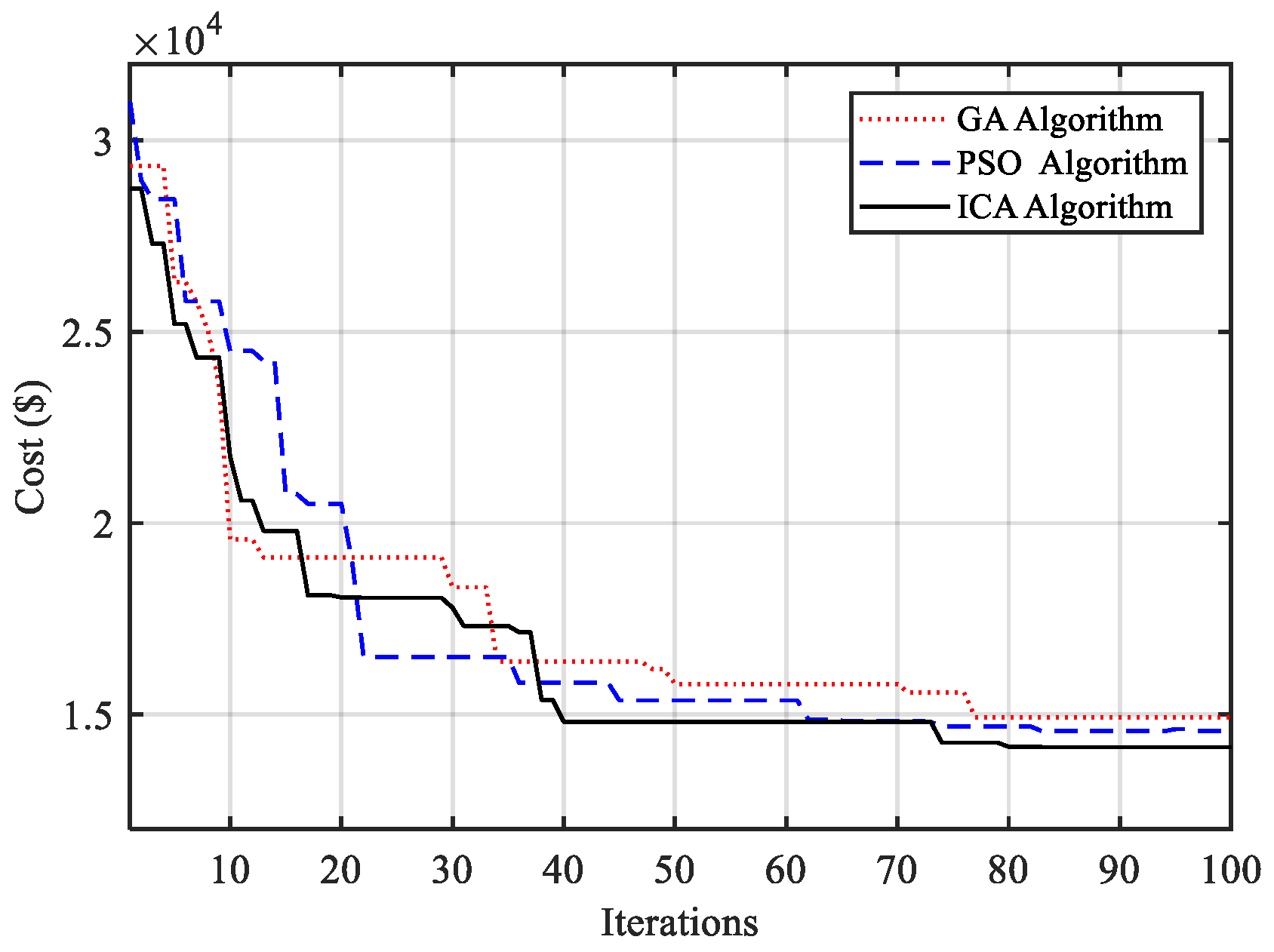
12], the authors have introduced a collaborative model of units in the presence of networkable electric vehicles by using a particle swarm optimization (PSO) algorithm to reduce the operation cost and the environmental emission in a MG. Also, in [13], scheduling DGs and scheduling charging and discharging EVs in a smart grid using the GAMS software was designed to reduce the cost of operating and emission rates. In [14] an energy management system (EMS) is proposed for residential microgrid (MG) with home parking lot based on the mixed integer linear program (MILP) method and for balancing power transactions in MG. The radial basis neural network (NN) method has been used to predict electrical demand. In this article, it is claimed that using car batteries parked in residential houses with proper management is an economical way to reduce operating costs. In [15], a model for maximizing the revenue from charging and discharging electric vehicles in the microgrid is proposed. The proposed model has de-peaked with the help of demand response program (DRP). The proposed method is implemented on the 14-bus IEEE system and the MILP optimization model is analyzed with CPLEX software. In [16], an online EMS is proposed for the optimal use of EVs in the parking lot in real time, and a balance between the demand and the state of charge (SOC) of the EV battery is obtained. The results of this paper show the efficiency of this method in supplying the loads with low operating costs.
Ignoring part of the operation cost of parking lots in the objective function to reduce optimization time by the algorithms and on the other hand being trapped in local optimal and low optimization convergence is the main drawbacks of the reviewed articles [17]. To increase the accuracy of the simulation results, a comprehensive objective function as well as the precise meta-heuristic algorithm should be used. The proposed algorithm should not be trapped in local optimum.
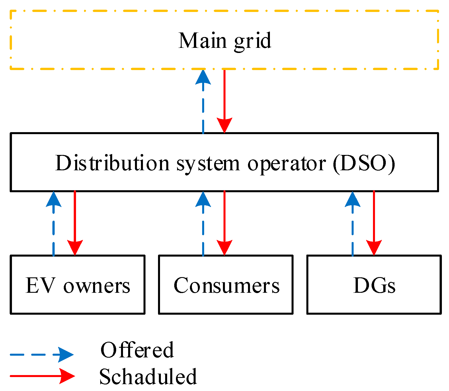
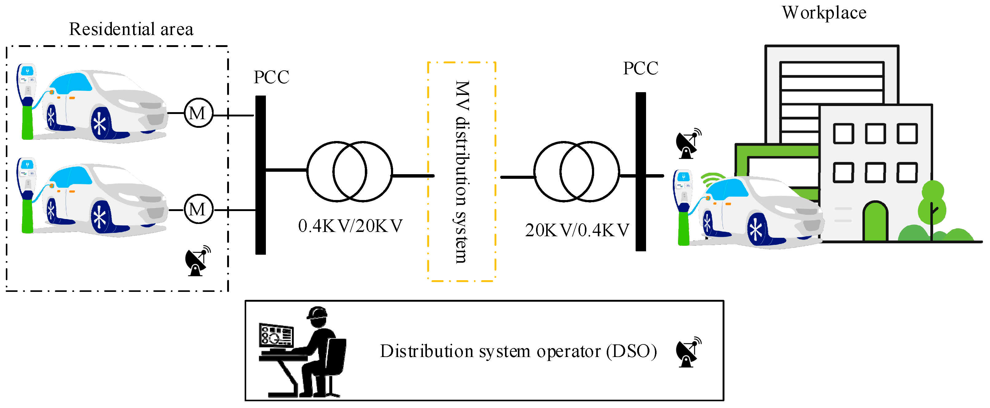
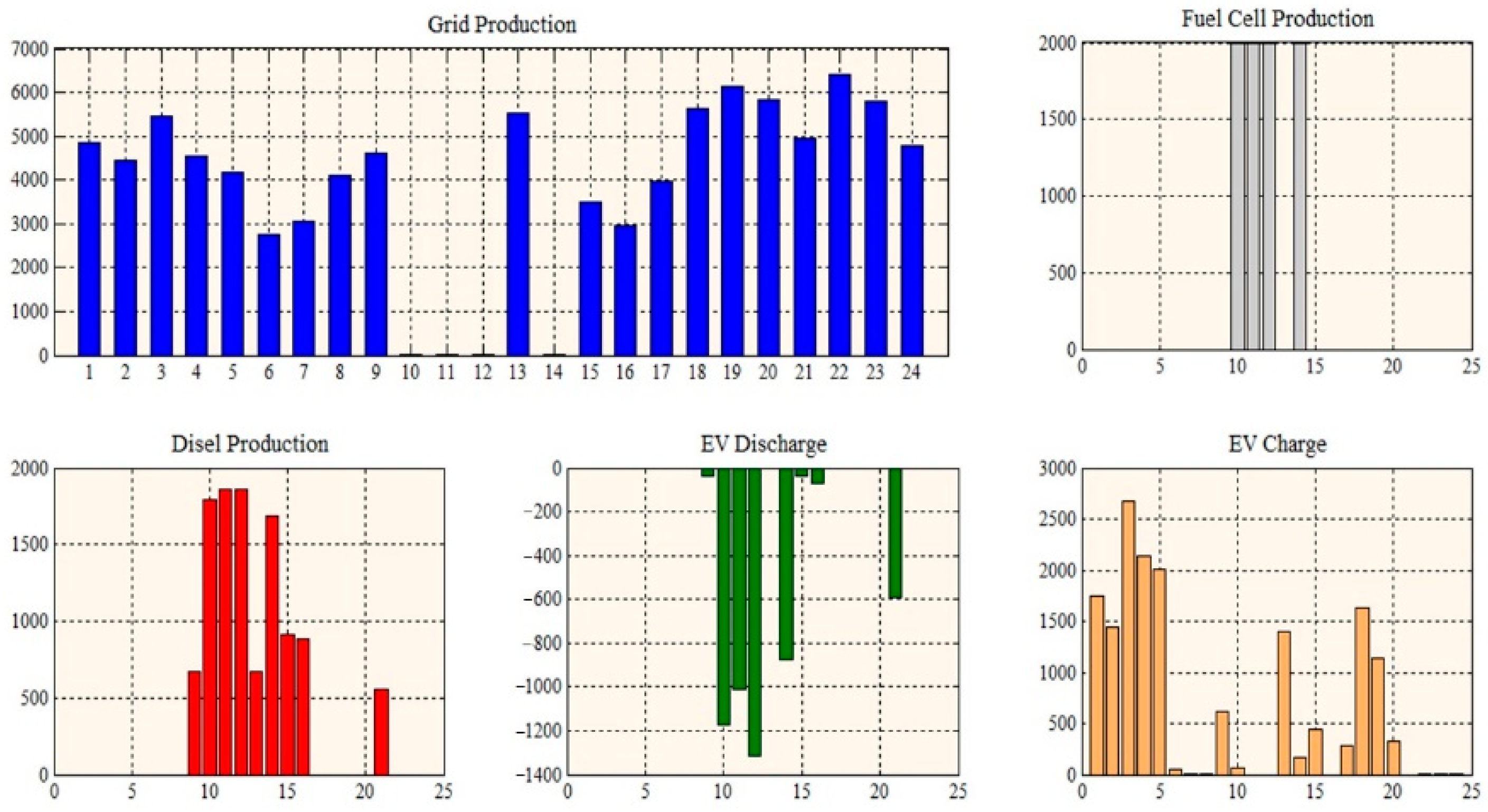
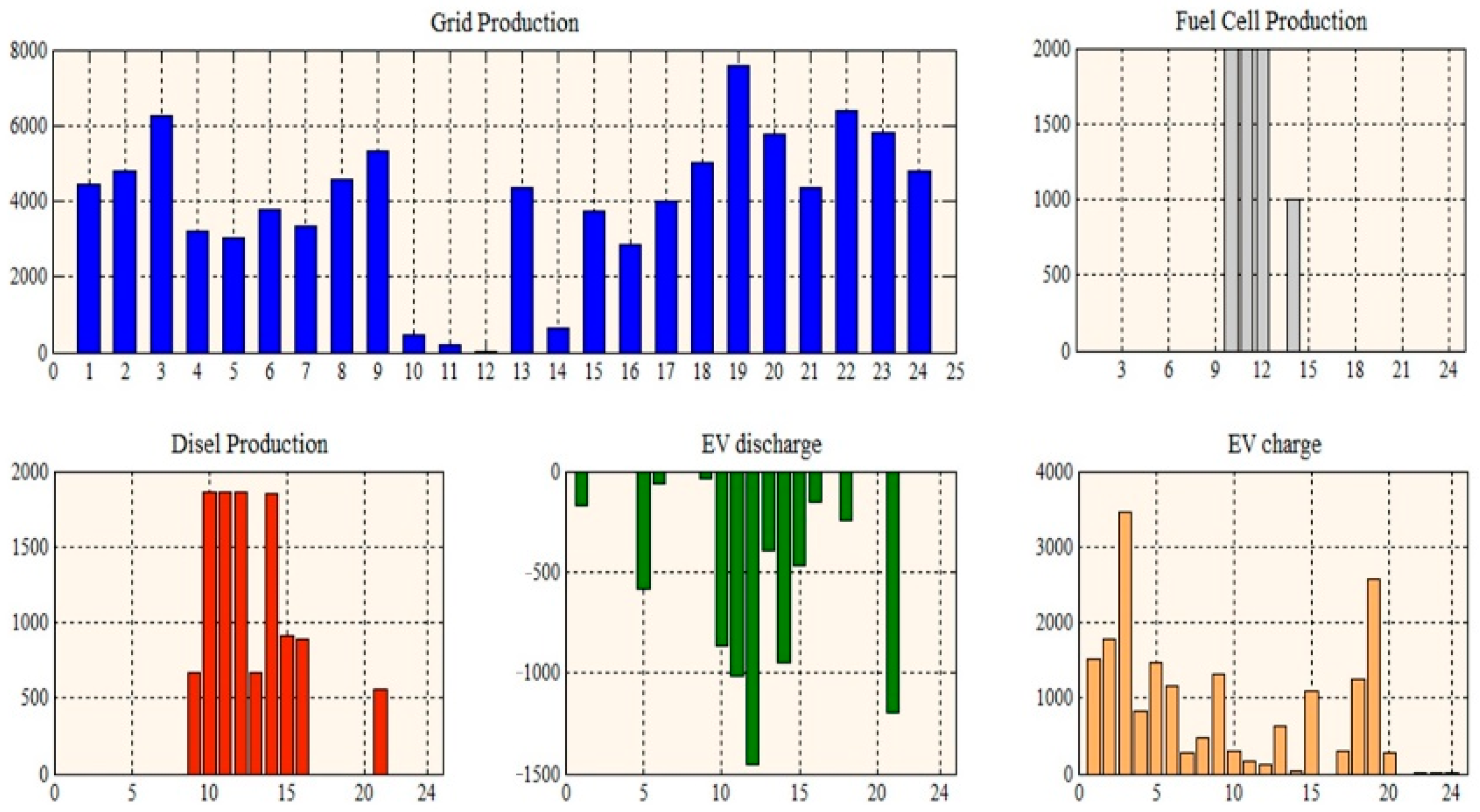
This paper specifically addresses the planning of the participation of distributed generation units and the scheduling of charging and discharging EV batteries during the 24 h for a day considering the vehicles daily schedule, which is received from the customer, to minimize the cost of the operation in consideration of the owners’ opinion. This issue is presented as an optimization problem with some constraints. In a smart grid environment, it is expected that the management of energy resources will be solved at a logical time, in spite of the operating constraints. Also, a modified version of the imperial competition algorithm is proposed to solve the optimization problem. High accuracy and not trapping in local optimal points are the prominent features of the proposed algorithm.

2. Smart Grid

In the proposed model, the distribution grid operator is responsible for planning the units in the distribution grid. The interaction between the distribution grid with its upstream and downstream portions is shown in Figure 1 [18].
The deployment of a smart grid requires the provision of the necessary infrastructure for the exchange of up-to-date information on the grid. The structure of the smart measurement system is considered to be a real project for the distribution grid arrangement, which can be seen in Figure 2 [19].
An identification chip (IC) is installed on each vehicle, which sends charging and discharging information for measurement by the meters, when the vehicle is connected to the grid. As depicted in the Figure 2, smart meter (SM) and power line carrier communication (PLCC) are installed at the consumer’s premises. This equipment can be single-phase or three-phase. Also, medium and large consumer measurements can transmit information through general packet radio system (GPRS). In addition, the electrical parameters of each feeder in the secondary post-distribution substation (63 kV/20 kV) are measured as distribution post (20 kV/0.4 kV) by the meters. By doing this, average pressure loss and low pressure can be calculated. Data concentrators (DCs) are installed at the place of distribution post transformers to manage all the data of the measured values in those sections. DCs send and information for meter data management and repository (MDM/R) for processing and preparation.
Electric vehicles must be integrated with other energy resources in the power grid and there should be a unit for integrating and coordinating vehicles and other sources of energy. This unit is called distribution management system (DMS). Electric vehicle management system (EVMS) is a subdivision of the DMS, which is responsible for managing the charging and discharging of vehicles in the smart grid. This unit receives vehicle information through MDM/R or customer information system (CIS). Magazine information to the graphical information system (GIS) is also transmitted via the CIS to the EVMS. In fact, the EVMS is responsible for keeping a database of vehicle information about their behavior and pattern before they can be charged or discharged. A vehicle owner can choose whether or not to participate in the charge and discharge plan. This agreement can be made through an internet portal. These connections are illustrated in Figure 3.

3. The Objective Function of the Problem

The formulas of the problem of planning power units and charging and discharging electric vehicles in the power grid are applicable for various purposes. Two objective functions are considered in this paper.

3.1. Cost Function without Vehicle Owners’ Opinion

The first objective function is the cost of the operator’s view, which is written as follows.
F cost = t = 1 T [ P g r i d ( t ) × Ω t + i = 1 N D G ( C D G ( i , t ) + S U ( i , t ) ) + v = 1 N P P E V D c h ( v , t ) × C D c h ( v , t ) + P L o s s ( t ) × Ω t + C O L T ]
In this formula P g r i d ( t ) and P L o s s ( t ) the power exchange with upstream network grid and power loss at time t, P E V D c h ( v , t ) is the electric power injected by the discharge of the electric vehicle and C D c h ( v , t ) is the price of electricity purchased by the vehicle’s owners, C D G ( i , t ) is the cost of producing each unit of diesel or fuel cell and S U ( i , t ) is their starting and shutdown cost, Ω t is electricity price in the market. Also, C O L T is transformer overload cost which is zero when the transformer is not overloaded. The DGs generation cost is derived from the following equation [20].
C D G ( i , t ) = a i × u ( i , t ) + b i × P D G ( i , t ) + c i × P 2 D G ( i , t )
where a i and, b i and, c i respectively are cost coefficients and P D G ( i , t ) is the ith DG cost at time t.

3.2. Cost Function with Vehicle Owners’ Opinion

Also, the goal function is related to cost from the viewpoint of vehicle owners, which is written as follows:
F cost = t = 1 T [ P g r i d ( t ) × Ω t + i = 1 T C D G ( i , t ) + S U ( i , t ) v = 1 N P P E V D c h ( v , t ) × C D c h v , t + P L o s s ( t ) × Ω t + C O L T ]
In this objective function, the vehicle owners’ profit resulted from the sale of electricity to the operator is as follows.
B e n e f i t = t = 1 T [ v = 1 N P P E V D c h ( v , t ) × C D c h v , t ]

3.3. Problem Constraints

Grid and DGs constraints and also constraints related to electric vehicles should be observed at any time of the day [13]. The main constraint for the grid is load balance constraint. It can be formulated as Equation (4). In which the total generation of the grid should be equal to the amount of consumption plus the losses in the grid.
P G r i d ( t ) + i = 1 N D G P D G i ( t ) + j = 1 N E V P E V _ D c h j ( t ) = D t + j = 1 N E V P E V _ c h j ( t ) + L o s s ( t ) ,
where, P E V _ c h j ( t ) and P E V _ D c h j ( t ) are the power charge and discharge of the jth EV, respectively; D t is the load demand, and L o s s ( t ) is the total power losses of power system during period t. Also, the voltage of all buses should not exceed the lower and upper limitations.
| v i min | | v i | | v i max |
In Equation (6), v i max and v i min are the upper and lower limitations of the bus voltage. Other constraints for the grid are the transmission line capacity limitations.
| I i j | | I i j max |
In Equation (7), I i j max is the maximum line flow capacity between buses i and j.
DGs generation capacity is the main constraint for these units. DGs have a capacity in rang of the minimum and maximum generation.
P i min P D G ( i , t ) P i max i { 1 , , I } ; t { 1 , , T }
where P i min and P i max are the bounds of the minimum and maximum output power ith of DG. If the minimum amount is lowered, that unit will be turned off and will need to pay again to set up [13].
{ U D G i ( t ) = 0 P D G i ( t ) < P D G _ M i n i U D G i ( t ) = 0 O W
In Equation (9), U D G i ( t ) is a binary value which is shown the ith DG is on or off. If P D G i ( t ) is lower than P D G _ M i n i will be turn off.
Electric vehicle (EV) charging and discharging constraints are as follows:
X ( v , t ) + Y ( v , t ) 1
where, X ( v , t ) and Y ( v , t ) are either zero or one at a time, respectively, to determine the discharge status and the charge of the batteries. This stipulates that every vehicle is charged or charged every time, either discharged or not charged or discharged [13].
E s ( v , t ) = E s ( v , t 1 ) P E V D c h ( v , t ) + P E V C h ( v , t ) E v , t t r i p
where E s ( v , t ) is the level of battery charge at the time t and E v , t t r i p is the amount of electric energy demand for having trip at time t. Also, P E V D c h ( v , t ) and P E V C h ( v , t ) are the amount of EVs charging and discharging rate respectively.
P E V D c h ( v , t ) P M A X D c h ( v , t ) × X ( v , t )
P E V C h ( v , t ) P M A X C h ( v , t ) × Y ( v , t )
Which states the charge and discharge rate of batteries per hour should not be higher than the virtual one.
E s ( v , t ) E M A X B a t , v
E s ( v , t ) E M I N B a t , v
Which states the remaining battery charge per hour should be within a permissible range [21].
P E V D c h ( v , t ) E s ( v , t 1 )
States that maximum amount of available charge per hour, each battery can give power to the grid.
P E V C h ( v , t ) E M A X B a t , v E s ( v , t 1 )
States that maximum amount of available capacity per hour, each battery can take power to the grid.
E s ( v , t l a s t q ) E T r i p , q v , t
States that each vehicle can use (move) eventually amount of available capacity on its battery [13].

4. Modified Imperialist Competitive Algorithm

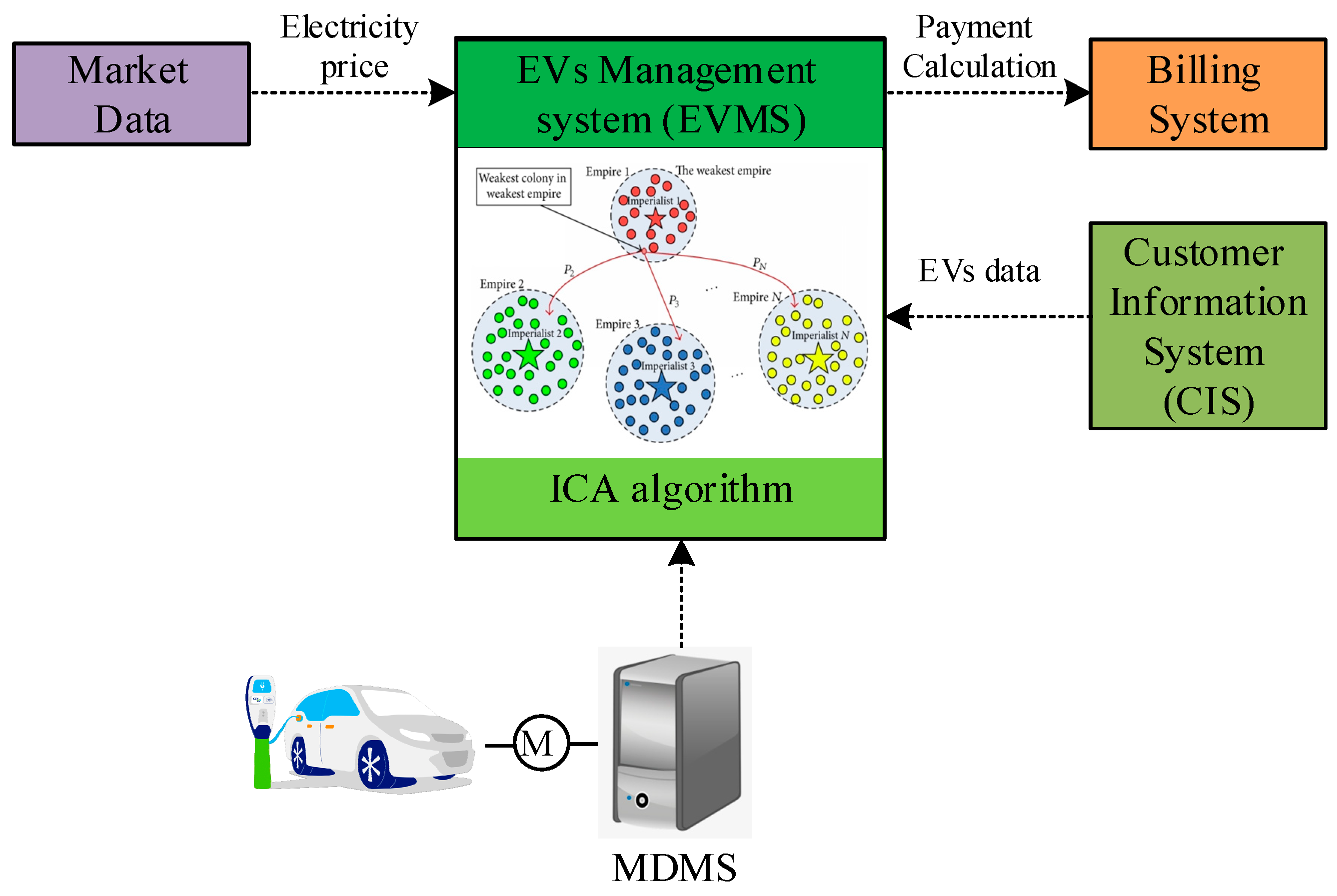
Imperial competition algorithm (ICA) was proposed by Caro Lucas and Esmael Atashpaz in 2008. This algorithm, similar to other algorithms, begins with a primitive population composed of a number of countries. To create empires, a number of the best countries are selected based on their deserving colonial qualities, and the rest of the countries are considered as their colony [22]. In an optimization problem with N variable, each country is constructed with an array 1 × N that is displayed as follows.
c o u n t r y = [ p 1 , p 2 , , p N ]
where p 1 ,   p 2 and p N are the variables of the problem. The value of the objective function is ith for the country is as follows.
c i = f ( c o u n t r y i ) = f ( P i 1 , P i 2 , , P i N )
To start the optimization process, the N country is created as a primary population. Then N i m p from these countries are selected as colonizers based on their worth. N c o l remaining countries are considered as a colony. Then, to create empires, the colonial colonies are divided by the power of each colonist. To divide them among colonists, first of all, the degree of plurality of colonizers must be normalized, which is done in the following way.
C n = c n max i { c i }
That c n is the value of the objective function for the colonizer and C n is its normalized value. Therefore, any colonialist whose value has a more objective function would have a lower normalized value. With the normalized value of the objective function for each colonizer, the power of each colonizer is calculated by the following equation [23,24,25,26,27,28,29,30,31,32,33,34,35,36,37,38,39,40,41,42,43,44,45,46,47,48,49,50,51,52,53,54,55,56,57,58,59,60,61].
p n = | C n i = 1 N i m p C i |
And finally, the colonial colony’s initial number is obtained from the following equation.
N C n = r o u n d   { p n · ( N c o l ) }
Which N C n is the n number colony of first colonists. For the division of colonies between empires, N C n are randomly selected from colonies and belong to the respective empire. Each empire that has more power will have a greater chance of absorbing the colony. The colonial countries are trying to advance their colonies. This fact is modeled by moving all the colonies towards their colonialist. This movement is modeled by two formulas, x and θ two random variables are distributed uniformly.
x ~ U ( 0 , β × d )
θ ~ U ( γ , γ )
In these formulas, x is the vector of the size and θ is the degree of deviation from the direction of movement towards the colonialist. Also, β is a number greater than 1, d is the distance between the colony and colonialist, Y is a parameter that determines the degree of diversion. As each colony moves toward the colonizer, that colony may acquire a lower cost function than its colonialist. Therefore, the role of the two will change together and the algorithm continues with the new colonizer. All other empires, on the strength of their power, are given the chance to seize the colony. So that, the power of each empire must be defined. First, the value of the cost function of each empire is calculated with the formula below [22].
T . C . n = Cost ( i m p e r i a l i s t n ) + ξ × m e a n { Cost ( c o l o n i e s o f e m p i r e s n ) }
In which, T . C . n , the total function of n empire cost, is a positive number less than 1. can determine the extent to which the colonies of each empire have the same value per ξ capita cost per empire than colonialism. Obviously, the values close to one, the effect of the colonies on the value of the function of the cost of the empire and the values close to zero will increase the colonial influence. After calculating the value of the cost function for each empire, these values are normalized to find the power of each empire as follows.
N . T . C . n = T . C . n max { T . C . i }
Which T . C . n and N . T . C . n are the value of the cost function and its normalized value for the nth of empire, respectively. With the normalization of the cost function of each empire, the probability of taking over, which represents the power of each empire, is obtained by Equation (28).
P P n = | N . T . C . n i = 1 N i m p N . T . C . i |
Thus, the following vector is defined that there is the possibility of seizing the colony for all the empire.
P = [ p p 1 , p p 2 , , p p n i m p ]
We then construct the vector-sized vector with the P vector called R whose arrays are random numbers with a uniform distribution between zero and one.
R = [ r 1 , r 2 , , r N i m p ]
Then the vector of subtraction of these two vectors is calculated as follows.
D = P R = [ D 1 , D 2 , , D N i m p ] = [ p p 1 r 1 , p p 2 r 2 , , p p n i m p r n i m p ]
Therefore, for each empire there is a vector in which each empire that has a larger value in this vector belongs to that colony. In the process of losing the colonies of weak empires, after all, all the empires will collapse except the empire that is strongest and all countries, as colonies, are under colonial control of this empire, and the absorption process is pursued with an existing empire so that the algorithm approaches the ideal conditions. In the proposed modified version of the ICA algorithm, it is supposed that in the weaker colonies, groups are formed and they try to improve the situation by making internal reforms. Internal reforms in colonies are variable in the form of random changes in the range of 10% of the upper and lower bands, which is expressed as Equation (32).
P = [ p p 1 , p p 2 , , p p n i m p ] × u n i f r n d ( 0.1 , 01 ) × ( U B L B )
where UB and 
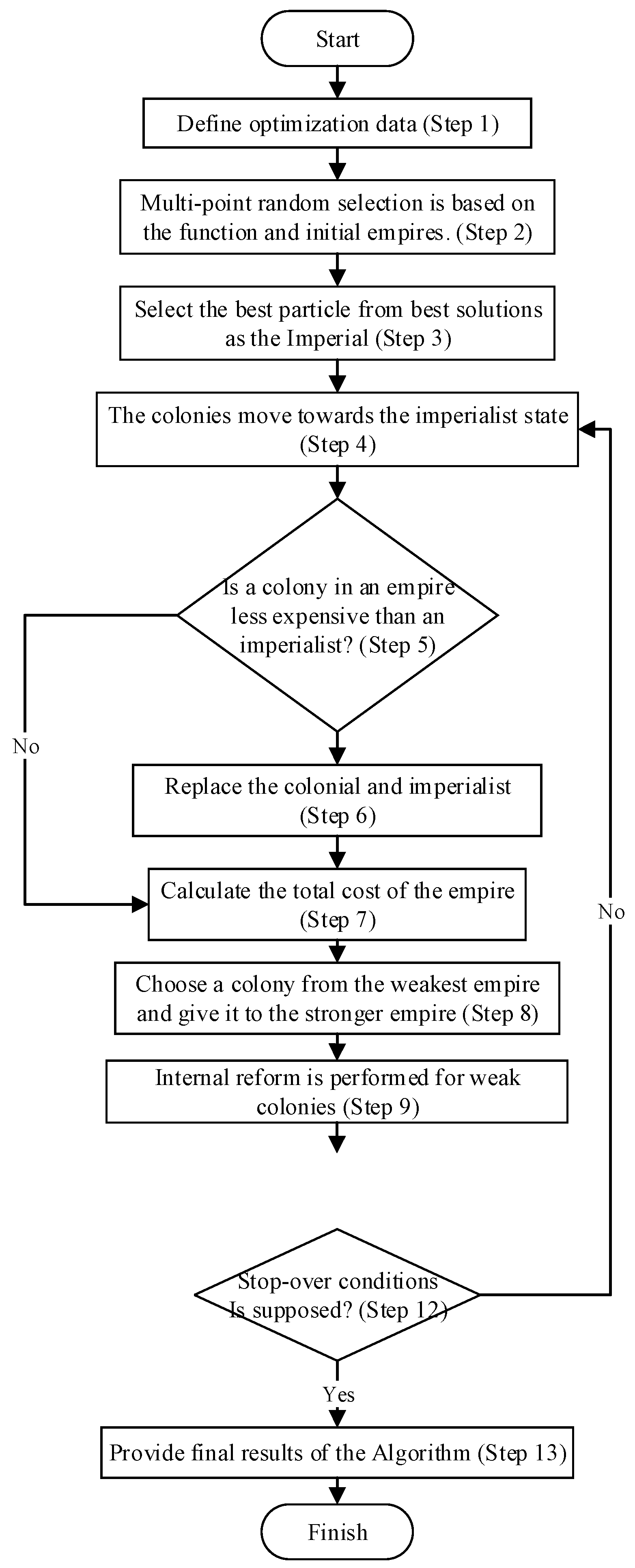
LB are upper and lower bounds respectively. The algorithm flowchart is shown in Figure 4.
Step 1: Define input data. These data include: cost of EVs and DGs operation, and also energy price, fuel cell parameters, diesel parameters and load level.
Step 2: Generate initial random population and calculate the objective functions (cost) for each country.
Step 3: Select the best particle from best solutions as the Imperial.
Step 4: Move the colonies to the imperialist country
Step 5: If there is a colony in the empire that costs less than the imperialist, replace the colonial and the imperialist together.
Step 6: Update the best position for each particle. To update the best position, the new particle position is compared with its previous position.
Step 7: Calculate the total cost of an empire (cost).
Step 8: Choose a colony from the weakest empire and give it to the empire most likely to be conquered.
Step 9: Internal reforms is performed for weak colonies.
Step 10: If the maximum number of iterations is reached, the optimization process stops, else returns to step 4.
Step 11: Remove the weak empires.
Step 12: If there is only one empire left, stop and go step 4.
Step 13: Provide final results of the Algorithm.

5. Case Study

The proposed approach to the modified version of the 33-buses radial distribution system has been implemented with a number of assumptions that changing these defaults could change the whole problem. For example, scheduling is based on a vehicle scheduling program that is fixed and announced in advance by the vehicle owners. In this planning, the length of time at home and at work and the duration of the journey for each vehicle are clear, and it is assumed that vehicles can only be recharged at home or at work. Also, for a vehicle battery, a maximum value and a first charge amount are considered. In this research, minimizing the cost from two perspectives has been investigated.

5.1. Assumptions and Problem Data

The predicted load profile of the test system for 24 h is shown in Figure 5.
The price of electricity in the free market is depicted in Table 1 [13]. It is also assumed that the electricity supplier purchases electricity at a constant price of 0.03 per 24 h from subscribers.
Also, two fuel cells and two diesel generators are installed in the buss (8, 19) and (27 and 13) respectively. The diesel generator and fuel cell are assumed to have a single power factor. Fuel price and fuel cell pollution rate and diesel generator are shown in Table 2 [13].
The electricity generated in the main network is supplied by fossil fuel-based power plants. The main network infiltration rate is 24 h (due to the switching and power offs of the above power plants) and is as shown in the Table 3 given below. A radial test system for a village is assumed to include industrial and commercial areas. The pattern is considered in accordance with reference [13]. This information includes the duration of travel for each type of vehicle, the start time and the end of travel, the average distance traveled.

5.2. The Behavioral Pattern of Vehicles Owners

The behavior of vehicles owners is grouped as follows:
-
Vehicle’s owners where their place of residence and work is in the village (types 1 and 2)
-
Vehicle’s owners where their place of residence is in the village and at work outside the village (types 3 and 4)
-
Vehicle’s owners where live in the village and use electric vehicles only to go shopping and party (type 5)
-
Planning to travel outside the city within certain timeframes (type 6)
-
They live out of town and they work in the city (Type 7).
Types 2 and 4 vehicles refer to vehicles that use their vehicles at dusk and at night for other jobs. In this research, two charging locations for vehicles are considered: (1) Charging at home (2) Charging at work. Pattern data for vehicles is shown in Table 3 and Table 4. The vehicle number and hours of start and end of their connection to the network are shown in Table 3 [13]. It’s assumed that the vehicles are moving at a constant rate and 3 kwh per hour consumes energy on average. The average travel period for each type of vehicle and the type of travel is given in Table 4 [13]. It should be noted that each type of vehicle stores enough energy in its battery to store the desired distance at an hour later. The data presented in Table 3 and Table 4 are standard data of test system parking lots.
In order to evaluate the optimization results, in addition to the proposed modified ICA algorithm, genetic algorithm (GA) and particle swarm optimization (PSO) algorithm are used for optimization and the results were compared with each other. The algorithms parameters are given in Table 5.

5.3. Vehicle Types in Terms of Battery Capacity

In this research, four different types of vehicles are considered, with a capacity of 10, 16, 24 and 40. Each vehicle owner chooses a particular type of vehicle according to their drive pattern. In addition, the initial charge rates for each battery are selected according to the running hours of each type, as shown in Table 6 [13].
Simulations are based on the fact that vehicles are only capable of charging at the home and workplace, and charging is not done outside of these two places and at parking lots. Battery chargers and converters have some losses, and thus, the amount of power received from the network is greater than the battery power. The battery charging and discharging efficiency is 90% and 95% respectively. In order to increase the battery life of electric vehicles, the maximum capacity can be up to 85% of the nominal capacity of the batteries. According to the standard equipment for charging and discharging vehicles, the charging and discharging rate of vehicles per hour is not more than 4 kilowatts per hour.

5.4. Types of Studied Scenarios

To analyze the effects of EV planning on cost reduction, the model proposed in this paper has been tested in two scenarios.

5.4.1. Scenario 1: Minimizing the Cost of Exploitation without Consideration of the Vehicle Owners’ Opinion

In this scenario, the cost of operation is considered as the objective function. The convergence diagram of the GA, PSO and the proposed ICA algorithms are shown in Figure 6.
The black solid line, blue dash-line and red dot-line are convergence curves of the ICA, PSO and GA algorithms respectively. As shown in Figure 6, the proposed ICA algorithm converges to a lower final value of than the other two algorithms. The ICA algorithm converged to 14,145 $ and the PSO and GA algorithms converged to 14,562 $ and 14,923 $ respectively. The optimization running time is calculated as 121 S for the GA, 136 S for the PSO 136 S and 116 S for the proposed ICA algorithm.
The planned active powers for the main grid, fuel cell, and diesel generator as well as vehicle charging and discharging programs for 24 h for the proposed ICA algorithm in the first scenario are shown in Figure 7.
According to these figures shown, the results suggest that vehicles are charged at low-power watches that are reasonable, and in high-power watches, which are discharged with regard to their battery capacity and motion, because of the price of the purchased electricity. It is fixed by the owner of the vehicle owners and is equal to 0.03, so it is logical to buy them in these hours of electricity, rather than be taken from the grid. It is also observed that diesel generator generates more hours than the fuel cell in the circuit, according to the generation cost function itself, because the generation cost of the generator is lower due to the cost function of the generator. Distribution system voltage profile is shown in Figure 8. As shown in this figure, the voltage amplitude of all buses in the 24 h is within the permitted range.

5.4.2. Scenario 2: Minimizing the Cost of Operation Considering the Vehicle Owners’ Opinion

In this scenario, the cost of operation with considering to maximizing profits for vehicle owners is considered. As it is clear from the formula of the objective function, the system operator should optimize the cost of network generation and distributed generation sources and discharging the vehicles in an optimum manner. So that, in addition to lowering the cost of exploitation, maximum profits will be generated for vehicle owners. The optimization algorithm results for the second scenario are shown in Figure 9.
Similar to the first scenario, the proposed ICA algorithm performed better than the PSO and GA algorithms and converged to a lower final value. The final values for the GA, PSO and ICA are 14,873 $, 14,432 $ and 14,015 $ respectively. For this scenario, the simulation running time is calculated as 120 S, 134 S and 115 S for the GA, PSO and ICA algorithms respectively. The planned active powers for the main grid, fuel cell, and diesel generator and charging and discharging vehicles for the proposed ICA algorithm in this scenario are shown in Figure 10.
Voltage profile for the second scenario is shown in Figure 11.
Figure 11 proves that in all conditions, the voltage amplitude is not out of range. The comparison between scenarios 1 and 2 is also given in Table 7. As outlined in the figures and tables, in Scenario 2, more vehicles are discharged, and as a result, the profits of vehicle owners from the sale of electricity have been increased. Also, the results indicate that the profit from the electricity sale is more when we used the proposed ICA algorithm for optimization. The profitability in the first scenario is calculated as 123.592 $, 136.678 $ and 153.592 $ for GA, PSO and ICA algorithms, respectively. Profit from electricity sales in the second scenario are 191.315 $ for GA, 204.308 $ for PSO and 227.808 $ for ICA.

6. Conclusions

In this paper, the daily production of the grid and distributed generation resources are scheduled and the scheduling of charging and discharging of vehicles around the clock is carried out according to the type of motion behavior received by the vehicle owners. This is an issue with a large number of complex constraints, which has been solved in a very large scale. A comprehensive objective function based on operation cost and EVs owner profitability is proposed for the energy management of the microgrid. This problem has been solved in 2 scenarios and the following results have been achieved. The presence of vehicles on the grid and their participation in network products has had a very important contribution to optimizing the functions involved. The vehicles are able to significantly reduce the cost of operating the system when it is needed. Also, if the operator of the system considers the vehicle owners at the time of discharging the vehicle, it will be good for the vehicle owners which increase their interest in the use of electric vehicles, which has a very positive impact on the cost of operation. Productive resources also contributed greatly to improving system performance and reduce operating costs, according to their generation cost functions. Fuel cell has less participation in power generation due to higher generation costs than diesel generators. The objective functions, constraints and the proposed ICA of this paper can be used for other microgrids with different topologies in future work. In this paper, the uncertainties are denied. Therefore, for future studies, generation and load uncertainties can be considered.

Author Contributions

Conceptualization, H.S., M.A.K., F.A., I.C. and K.E.; Data curation, H.S., M.A.K. and K.E.; Formal analysis, H.S., M.A.K., F.A., I.C. and K.E.; Funding acquisition, H.S., M.A.K., F.A., I.C. and K.E.; Investigation, H.S., M.A.K. and F.A.; Methodology, H.S., M.A.K., F.A., I.C. and K.E.; Project administration, H.S. and M.A.K.; Resources, H.S., M.A.K., F.A. and I.C.; Software, H.S. and M.A.K.; Supervision, M.A.K.; Validation, M.A.K.; Writing–original draft, H.S. and M.A.K.; Writing–review & editing, I.C. and K.E. All authors have read and agreed to the published version of the manuscript.

Funding

This research received no external funding.

Institutional Review Board Statement

Not applicable.

Informed Consent Statement

Not applicable.

Data Availability Statement

Not applicable.

Conflicts of Interest

The authors declare no conflict of interest.

References

  1. Ghadi-Sahebi, M.; Ebrahimi, R.; Parvin-darabad, V. Optimal probabilistic operation management of smart parking lot and renewable sources in microgrid to reduce cost and improve system reliability considering demand response program. Int. Trans. Electron. Energy Syst. 2021, 31, 13108. [Google Scholar] [CrossRef]
  2. Hosseini Imani, M.; Jabbari Ghadi, M.; Shamshirband, S.; Balas, M.M. Impact evaluation of electric vehicle parking on solving security-constrained unit commitment problem. Math. Comput. Appl. 2018, 23, 13. [Google Scholar] [CrossRef] [Green Version]
  3. Shokouhandeh, H.; Jazaeri, M. An enhanced and auto-tuned power system stabilizer based on optimized interval type-2 fuzzy PID scheme. Int. Trans. Electron. Energy Syst. 2018, 28, 2469. [Google Scholar] [CrossRef]
  4. Cao, J.; Bu, Z.; Wang, Y.; Yang, H.; Jiang, J.; Li, H.J. Detecting prosumer-community groups in smart grids from the multiagent perspective. IEEE Trans. Syst. Man Cybern. Syst. 2019, 49, 1652–1664. [Google Scholar] [CrossRef]
  5. Shokouhandeh, H.; Ahmadi Kamarposhti, M.; Colak, I.; Eguchi, K. Unit Commitment for Power Generation Systems Based on Prices in Smart Grid Environment Considering Uncertainty. Sustainability 2021, 13, 10219. [Google Scholar] [CrossRef]
  6. Qu, Z.; Song, J.; Liu, Y.; Lv, H.; Hu, K.; Sun, J.; Wang, W. Optimization Model of EV Charging and Discharging Price Considering Vehicle Owner Response and Power Grid Cost. J. Electron. Eng. Technol. 2019, 14, 2251–2261. [Google Scholar] [CrossRef] [Green Version]
  7. Sousa, T.; Morais, H.; Vale, Z.; Faria, P.; Soares, J. Intelligent energy resource management considering vehicle-to-grid: A simulated annealing approach. IEEE Trans. Smart Grid 2012, 3, 535–542. [Google Scholar] [CrossRef]
  8. Hosseini, S.; Sarder, M.D. Development of a Bayesian network model for optimal site selection of electric vehicle charging station. Int. J. Electron. Power Energy Syst. 2019, 105, 110–122. [Google Scholar] [CrossRef]
  9. Venayagamoorthy, G.K. Dynamic, stochastic, computational, and scalable technologies for smart grids. IEEE Comput. Intell. Mag. 2011, 6, 22–35. [Google Scholar] [CrossRef]
  10. Soares, J.; Morais, H.; Sousa, T.; Vale, Z.; Faria, P. Day-ahead resource scheduling including demand response for electric vehicles. IEEE Trans. Smart Grid 2013, 4, 596–605. [Google Scholar] [CrossRef] [Green Version]
  11. Deilami, S.; Masoum, A.S.; Moses, P.S.; Masoum, M.A. Real-time coordination of plug-in electric vehicle charging in smart grids to minimize power losses and improve voltage profile. IEEE Trans. Smart Grid 2011, 2, 456–467. [Google Scholar] [CrossRef]
  12. Cheng, H.; Luo, T.; Kang, C.; Xin, J.; Wan, H.; Pei, F.; Tian, X. An Interactive Strategy of Grid and Electric Vehicles Based on Master-Slaves Game Model. J. Electron. Eng. Technol. 2020, 15, 299–306. [Google Scholar] [CrossRef]
  13. Ko, Y.S.; Ryu, K.; Oh, M.S.; Yoon, H.S. A Study on the Miniaturization of a Protective Device for the Micro Smart Grid Simulator. J. Electron. Eng. Technol. 2020, 15, 85–94. [Google Scholar] [CrossRef]
  14. Muthiah-Nakarajan, V.; Cherukuri, S.H.C.; Saravanan, B.; Palanisamy, K. Residential energy management strategy considering the usage of storage facilities and electric vehicles. Sustain. Energy Technol. Assess. 2021, 45, 101167. [Google Scholar] [CrossRef]
  15. Liu, Z.; Li, P.; Liu, J.; He, X.; Han, J.; Zi, C.; Liang, N. A day-ahead energy management and reserve declaration strategy for parking lot based on electric vehicle accessing guidance. Int. J. Electron. Power Energy Syst. 2022, 136, 107704. [Google Scholar] [CrossRef]
  16. Lotfi, M.; Almeida, T.; Javadi, M.S.; Osório, G.J.; Monteiro, C.; Catalão, J.P. Coordinating energy management systems in smart cities with electric vehicles. Appl. Energy 2022, 307, 118241. [Google Scholar] [CrossRef]
  17. Zahraoui, Y.; Alhamrouni, I.; Mekhilef, S.; Basir Khan, M.R.; Seyedmahmoudian, M.; Stojcevski, A.; Horan, B. Energy Management System in Microgrids: A Comprehensive Review. Sustainability 2021, 13, 10492. [Google Scholar] [CrossRef]
  18. Cecati, C.; Citro, C.; Siano, P. Combined operations of renewable energy systems and responsive demand in a smart grid. IEEE Trans. Sustain. Energy 2011, 2, 468–476. [Google Scholar] [CrossRef]
  19. Bhargavi, K.M.; Jayalakshmi, N.S. A new control strategy for plug-in electric vehicle of DC microgrid with PV and wind power integration. J. Electron. Eng. Technol. 2019, 14, 13–25. [Google Scholar] [CrossRef]
  20. Shokouhandeh, H.; Ghaharpour, M.; Lamouki, H.G.; Pashakolaei, Y.R.; Rahmani, F.; Imani, M.H. Optimal estimation of capacity and location of wind, solar and fuel cell sources in distribution systems considering load changes by lightning search algorithm. In Proceedings of the 2020 IEEE Texas Power and Energy Conference (TPEC), College Station, TX, USA, 6–7 February 2020. [Google Scholar]
  21. Byun, J.; Kim, M.; Joo, D.; Lee, W.Y.; Choe, G.Y.; Lee, B.K. Frequency and Phase-Shift Control of Inductive Power Transfer for EV Charger with LCCL-S Resonant Network Considering Misalignment. J. Electron. Eng. Technol. 2019, 14, 2409–2419. [Google Scholar] [CrossRef]
  22. Yu, H.; Li, J.Q.; Zhang, L.; Duan, P. An imperialist competition algorithm using a global search strategy for physical examination scheduling. Appl. Intell. 2021, 51, 3936–3951. [Google Scholar] [CrossRef] [PubMed]
  23. Zhao, T.-H.; Castillo, O.; Jahanshahi, H.; Yusuf, A.; Alassafi, M.O.; Alsaadi, F.E.; Chu, Y.-M. A fuzzy-based strategy to suppress the novel coronavirus (2019-NCOV) massive outbreak. Appl. Comput. Math. 2021, 20, 160–176. [Google Scholar]
  24. Zhao, T.-H.; Wang, M.-K.; Chu, Y.-M. On the bounds of the perimeter of an ellipse. Acta Math. Sci. 2022, 42B, 491–501. [Google Scholar] [CrossRef]
  25. Zhao, T.-H.; Wang, M.-K.; Hai, G.-J.; Chu, Y.-M. Landen inequalities for Gaussian hypergeometric function. Rev. R. Acad. Cienc. Exactas Fis. Nat. Ser. A Mat. RACSAM 2021, 116, 23. [Google Scholar] [CrossRef]
  26. Nazeer, M.; Hussain, F.; Khan, M.I.; ur-Rehman, A.; El-Zahar, E.R.; Chu, Y.-M.; Malik, M.Y. Theoretical study of MHD electro-osmotically flow of third-grade fluid in micro channel. Appl. Math. Comput. 2021, 420, 126868. [Google Scholar] [CrossRef]
  27. Chu, Y.-M.; Shankaralingappa, B.M.; Gireesha, B.J.; Alzahrani, F.; Khan, M.I.; Khan, S.U. Combined impact of Cattaneo-Christov double diffusion and radiative heat flux on bio-convective flow of Maxwell liquid configured by a stretched nano-material surface. Appl. Math. Comput. 2021, 419, 126883. [Google Scholar] [CrossRef]
  28. Zhao, T.-H.; Khan, M.I.; Chu, Y.-M. Artificial neural networking (ANN) analysis for heat and entropy generation in flow of non-Newtonian fluid between two rotating disks. Math. Methods Appl. Sci. 2021. [Google Scholar] [CrossRef]
  29. Iqbal, M.A.; Wang, Y.; Miah, M.M.; Osman, M.S. Study on Date–Jimbo–Kashiwara–Miwa Equation with Conformable Derivative Dependent on Time Parameter to Find the Exact Dynamic Wave Solutions. Fractal Fract. 2022, 6, 4. [Google Scholar] [CrossRef]
  30. Zhao, T.-H.; He, Z.-Y.; Chu, Y.-M. Sharp bounds for the weighted Holder mean of the zero-balanced generalized complete elliptic integrals. Comput. Methods Funct. Theory 2021, 21, 413–426. [Google Scholar] [CrossRef]
  31. Zhao, T.-H.; Wang, M.-K.; Chu, Y.-M. Concavity and bounds involving generalized elliptic integral of the first kind. J. Math. Inequal. 2021, 15, 701–724. [Google Scholar] [CrossRef]
  32. Zhao, T.-H.; Wang, M.-K.; Chu, Y.-M. Monotonicity and convexity involving generalized elliptic integral of the first kind. Rev. R. Acad. Cienc. Exactas Fis. Nat. Ser. A Mat. RACSAM 2021, 115, 13. [Google Scholar] [CrossRef]
  33. Chu, H.-H.; Zhao, T.-H.; Chu, Y.-M. Sharp bounds for the Toader mean of order 3 in terms of arithmetic, quadratic and contraharmonic means. Math. Slovaca 2020, 70, 1097–1112. [Google Scholar] [CrossRef]
  34. Zhao, T.-H.; He, Z.-Y.; Chu, Y.-M. On some refinements for inequalities involving zero-balanced hypergeometric function. AIMS Math. 2020, 5, 6479–6495. [Google Scholar] [CrossRef]
  35. Zhao, T.-H.; Wang, M.-K.; Chu, Y.-M. A sharp double inequality involving generalized complete elliptic integral of the first kind. AIMS Math. 2020, 5, 4512–4528. [Google Scholar] [CrossRef]
  36. Zhao, T.-H.; Shi, L.; Chu, Y.-M. Convexity and concavity of the modified Bessel functions of the first kind with respect to Holder means. Rev. R. Acad. Cienc. Exactas Fis. Nat. Ser. A Mat. RACSAM 2020, 114, 14. [Google Scholar] [CrossRef]
  37. Zhao, T.-H.; Zhou, B.-C.; Wang, M.-K.; Chu, Y.-M. On approximating the quasi-arithmetic mean. J. Inequal. Appl. 2019, 2019, 12. [Google Scholar] [CrossRef]
  38. Zhao, T.-H.; Wang, M.-K.; Zhang, W.; Chu, Y.-M. Quadratic transformation inequalities for Gaussian hypergeometric function. J. Inequal. Appl. 2018, 2018, 251. [Google Scholar] [CrossRef] [Green Version]
  39. Chu, Y.-M.; Zhao, T.-H. Concavity of the error function with respect to Holder means. Math. Inequal. Appl. 2016, 19, 589–595. [Google Scholar] [CrossRef]
  40. Zhao, T.-H.; Shen, Z.-H.; Chu, Y.-M. Sharp power mean bounds for the lemniscate type means. Rev. R. Acad. Cienc. Exactas Fis. Nat. Ser. A Mat. RACSAM 2021, 115, 16. [Google Scholar] [CrossRef]
  41. Song, Y.-Q.; Zhao, T.-H.; Chu, Y.-M.; Zhang, X.-H. Optimal evaluation of a Toader-type mean by power mean. J. Inequal. Appl. 2015, 2015, 408. [Google Scholar] [CrossRef] [Green Version]
  42. Chu, Y.-M.; Zhao, T.-H. Convexity and concavity of the complete elliptic integrals with respect to Lehmer mean. J. Inequal. Appl. 2015, 2015, 396. [Google Scholar] [CrossRef] [Green Version]
  43. Zhao, T.-H.; Yang, Z.-H.; Chu, Y.-M. Monotonicity properties of a function involving the psi function with applications. J. Inequal. Appl. 2015, 193, 10. [Google Scholar] [CrossRef] [Green Version]
  44. Chu, Y.-M.; Wang, H.; Zhao, T.-H. Sharp bounds for the Neuman mean in terms of the quadratic and second Seiffert means. J. Inequal. Appl. 2014, 299, 14. [Google Scholar] [CrossRef] [Green Version]
  45. Sun, H.; Zhao, T.-H.; Chu, Y.-M.; Liu, B.-Y. A note on the Neuman-Sandor mean. J. Math. Inequal. 2014, 8, 287–297. [Google Scholar] [CrossRef] [Green Version]
  46. Chu, Y.-M.; Zhao, T.-H.; Liu, B.-Y. Optimal bounds for Neuman-Sandor mean in terms of the convex combination of logarithmic and quadratic or contra-harmonic means. J. Math. Inequal. 2014, 8, 201–217. [Google Scholar] [CrossRef] [Green Version]
  47. Chu, Y.-M.; Zhao, T.-H.; Song, Y.-Q. Sharp bounds for Neuman-Sandor mean in terms of the convex combination of quadratic and first Seiffert means. Acta Math. Sci. 2014, 34B, 797–806. [Google Scholar] [CrossRef]
  48. Zhao, T.-H.; Chu, Y.-M.; Jiang, Y.-L.; Li, Y.-M. Best possible bounds for Neuman-Sandor mean by the identric, quadratic and contraharmonic means. Abstr. Appl. Anal. 2013, 2013, 348326. [Google Scholar] [CrossRef] [Green Version]
  49. Zhao, T.-H.; Chu, Y.-M.; Liu, B.-Y. Optimal bounds for Neuman-Sandor mean in terms of the convex combinations of harmonic, geometric, quadratic, and contraharmonic means. Abstr. Appl. Anal. 2012, 2012, 1–9. [Google Scholar] [CrossRef]
  50. Wang, M.-K.; Hong, M.-Y.; Xu, Y.-F.; Shen, Z.-H.; Chu, Y.-M. Inequalities for generalized trigonometric and hyperbolic functions with one parameter. J. Math. Inequal. 2020, 14, 1–21. [Google Scholar] [CrossRef]
  51. Xu, H.-Z.; Qian, W.-M.; Chu, Y.-M. Sharp bounds for the lemniscatic mean by the one-parameter geometric and quadratic means. Rev. R. Acad. Cienc. Exactas Fis. Nat. Ser. A Mat. RACSAM 2022, 116, 15. [Google Scholar] [CrossRef]
  52. Karthikeyan, K.; Karthikeyan, P.; Baskonus, H.M.; Venkatachalam, K.; Chu, Y.-M. Almost sectorial operators on Psi-Hilfer derivative fractional impulsive integro-differential equations. Math. Methods Appl. Sci. 2021. [Google Scholar] [CrossRef]
  53. Chu, Y.-M.; Nazir, U.; Sohail, M.; Selim, M.M.; Lee, J.-R. Enhancement in thermal energy and solute particles using hybrid nanoparticles by engaging activation energy and chemical reaction over a parabolic surface via finite element approach. Fractal Fract. 2021, 5, 119. [Google Scholar] [CrossRef]
  54. Rashid, S.; Sultana, S.; Karaca, Y.; Khalid, A.; Chu, Y.-M. Some further extensions considering discrete proportional fractional operators. Fractals 2022, 30, 2240026. [Google Scholar] [CrossRef]
  55. Zhao, T.-H.; Qian, W.-M.; Chu, Y.-M. Sharp power mean bounds for the tangent and hyperbolic sine means. J. Math. Inequal. 2021, 15, 1459–1472. [Google Scholar] [CrossRef]
  56. Zhao, T.-H.; Qian, W.-M.; Chu, Y.-M. On approximating the arc lemniscate functions. Ind. J. Pure Appl. Math. 2021, 74. [Google Scholar] [CrossRef]
  57. Hajiseyedazizi, S.N.; Samei, M.E.; Alzabut, J.; Chu, Y.-M. on multi-step methods for singular fractional q-integro-differential equations. Open Math. 2021, 19, 1–28. [Google Scholar] [CrossRef]
  58. He, Z.-Y.; Abbes, A.; Jahanshahi, H.; Alotaibi, N.D.; Wang, Y. Fractional-order discrete-time SIR epidemic model with vaccination: Chaos and complexity. Mathematics 2022, 10, 165. [Google Scholar] [CrossRef]
  59. Jin, F.; Qian, Z.-S.; Chu, Y.-M.; ur Rahman, M. On nonlinear evolution model for drinking behavior under Caputo-Fabrizio derivative. J. Appl. Anal. Comput. 2022, 12, 790–806. [Google Scholar] [CrossRef]
  60. Rashid, S.; Abouelmagd, E.I.; Khalid, A.; Farooq, F.B.; Chu, Y.-M. Some recent developments on dynamical hbar-discrete fractional type inequalities in the frame of nonsingular and nonlocal kernels. Fractals 2022, 30, 2240110. [Google Scholar] [CrossRef]
  61. Wang, F.-Z.; Khan, M.N.; Ahmad, I.; Ahmad, H.; Abu-Zinadah, H.; Chu, Y.-M. Numerical solution of traveling waves in chemical kinetics: Time-fractional fishers equations. Fractals 2022, 30, 22400051. [Google Scholar] [CrossRef]
Figure 1. Interaction between the DSO and the upper and lower parts.
Sustainability 14 04770 g001
Figure 2. Smart Grid Structure.
Sustainability 14 04770 g002
Figure 3. Diagram of the electric vehicle management system.
Sustainability 14 04770 g003
Figure 4. The proposed ICA algorithm flowchart.
Sustainability 14 04770 g004
Figure 5. Grid load profiles in 24 h.
Sustainability 14 04770 g005
Figure 6. Convergence curves of problem solving for scenario 1.
Sustainability 14 04770 g006
Figure 7. 24-h scheduling of main grid generation, fuel cell and diesel generator and charging and discharging of vehicles in scenario 1.
Sustainability 14 04770 g007
Figure 8. Voltage profile in scenario 1.
Sustainability 14 04770 g008
Figure 9. Convergence curves of problem solving for scenario 2.
Sustainability 14 04770 g009
Figure 10. 24-h scheduling of main grid generation, fuel cell and diesel generator and charging and discharging vehicles in scenario 2.
Sustainability 14 04770 g010
Figure 11. Voltage profile in scenario 2.
Sustainability 14 04770 g011
Table 1. Price of electricity on the free market.
t123456789101112
$/kwh0.0330.0270.020.0170.0170.0290.0330.0540.2150.5720.5720.572
t131415161718192021222324
$/kwh0.2150.5720.2860.2790.0860.0590.050.0610.1810.0770.0430.037
Table 2. Specifications for distributed generation.
Power StationCost Function CoefficientsGeneration Limit
a ($)b ($)c ($)Startup ($)Pmin (Kw) Pmax (Kw)
Diesel100.01330.00032501000
Fuel cell450.375 31001000
Table 3. Presence hours of vehicles at home and at workplace.
Vehicle TypeNumberStop Time
HomeWorkplace
12001–6, 17–248–15
22001–6, 17–198–15
31001–5, 17–24-
42001–5, 17–19-
51501–9, 13–18, 22–24-
6100-8–15
7501–6-
Table 4. Average travel times.
Vehicle Type Move Type/Duration of Movement
From Home to WorkplaceFrom Workplace to HomeOthers
111-
2115
322-
4225
5--3&3
622-
7--10
Table 5. The algorithms parameters.
GAPopulationIterationPmPc
1201000.250.8
ICAPopulationIterationAβζ
1201000.041.70.1
PSOPopulationIterationC1 = C2VmaxVminW
13010020.90.40.7
Table 6. The amount of battery capacity of each vehicle type.
Vehicle TypeBattery Capacity (KWh)Initial Battery Charge
Type of 1–3–6104
Type of 5168
Type of 2–42412
Type of 74025
Table 7. Comparison between vehicle discharging and sales profit in scenarios 1 and 2.
Discharging Vehicles Rate (kW)Profit from Electricity Sales ($)
GAScenario 15073.5123.592
Scenario 27465.2191.315
PSOScenario 15091.6 136.678
Scenario 27503.1204.308
ICAScenario 15119.7153.592
Scenario 27593.6227.808
Publisher’s Note: MDPI stays neutral with regard to jurisdictional claims in published maps and institutional affiliations.

