Article

Influences of Environmental Regulations on Industrial Green Technology Innovation Efficiency in China

1
Shandong Key Laboratory of Blockchain Finance, Shandong University of Finance and Economics, Jinan 250014, China
2
School of Mathematics and Quantitative Economics, Shandong University of Finance and Economics, Jinan 250002, China
3
Shandong Technology Innovation Center of Social Governance Intelligence, Shandong University of Finance and Economics, Jinan 250014, China
4
Kent Business School, University of Kent, Canterbury CT1 7NZ, UK
5
Centre for Evaluation Studies, Beijing Normal University, Zhuhai 519088, China
6
Division of Business and Management, Beijing Normal University, Hong Kong Baptist University United International College, Zhuhai 519087, China
*
Author to whom correspondence should be addressed.
Sustainability 2022, 14(8), 4717; https://doi.org/10.3390/su14084717
Submission received: 4 March 2022 / Revised: 4 April 2022 / Accepted: 12 April 2022 / Published: 14 April 2022

Abstract

:
The Paris Agreement marks global response to climate change after 2020 and China has proposed the dual carbon goals, carbon peaking and carbon neutrality, in response. This paper analyses the contribution to dual carbon goals by analyzing the impact of environmental regulations (ERs) on green technology innovation (GTI) in China. First, considering variances in energy consumption structure across provinces and industries, industrial CO2 emission is calculated and set as an undesirable output of industrial GTI. Then, industrial green technology innovation efficiencies (GTIE) of 29 provinces in China between 2005–2017 are calculated using a non-oriented two-stage network SBM-DEA model assuming variable returns to scale. Last, dynamic evolution and regional differences of industrial GTIE during green technology R&D, green technology commercialization, and overall GTI stages are respectively observed, and the influences from different types of ERs, command-based (CER), market-based (MER), and voluntary (VER), on industrial GTIE are analyzed. We identify China is overall experiencing relatively low but gradually increasing industrial GTIE and Industrial GTIE present gradient changes across provinces with increasingly prominent regional difference. It is found that influences of types of ERs on industrial GTIE present dynamic effect, threshold effect, lag effect and regional differences.

1. Introduction

China marched greatly towards industrialization and urbanization during the 13th Five-Year planning under the Paris Agreement and strategically introduced the dual carbon goals. While proceeding in ecology and culture construction, China is facing environmental issues including resource consumption, carbon dioxide (CO2) emission, and waste pollutant accumulation [1], which hindered social sustainable development with extensive increase in high investment, high energy consumption, and high emission. Referring to China Statistical Yearbook on Environment, in 2019, industrial Sulphur dioxide (SO2) emission reached 3.954 million tons, industrial solid waste reached 4.49 million tons, and overall industrial emission of oxygen demand for chemicals was 77.2 tons [2]. Generally, industrial emission takes the greatest proportion of carbon emissions for about 70% of the China’s total annual [3]. President Xi Jinping pointed out at the National Conference on Innovation in Science and Technology that ecology and culture development faces increasingly serious environmental pollution and needs to rely on green technology innovation (GTI) for green development and build a beautiful China with blue sky, green land and clear water [4]. As a new way of innovation, GTI not only pays attention to the economic growth highlighted by traditional innovation, but also concentrates on resource-saving and environmental protection such as reducing CO2 emissions [5,6]. However, due to high externalities and high innovation cost, some firms lack motivations for GTI [7]. Higher level of GTI is a response to the Paris Agreement and the United Nations Sustainable Development Goals (SDGs).
Among many factors influencing GTI, ‘Porter hypothesis’ claims that in the long run, environmental regulations (ERs) may positively promote GTI, forming “innovation compensation effect” [8]. ER is a constraining force that provides external incentives for industry to adjust its production methods to protect the environment [9]. It is now popularly classified to three types, command-based environmental regulation (CER), market-based environmental regulation (MER), and voluntary environmental regulation (VER) [9]. They are differentiated according to the key actors of each type which are the government, the enterprises and the citizens respectively. Given new economic norms and high-quality economic development promoted by the government, the Chinese government has issued a series of ERs. On 1 January 2018, China’s environmental protection tax law was officially implemented, aiming to promote the construction of ecological civilization. On such basis, we recognize the necessity to delve into the influences of different types of ERs to GTI to improve towards industrial green transformation and upgrading and the dual carbon targets.
While extensive research is done around the impact of ER on GTI, studies are limited in using green technology innovation efficiency (GTIE) as the GTI process proxy. Although results can be different due to the selection of indicators and method and varied regional environment, economy, and administrative management, most of them indicate the influence of ER on GTI will be positive, negative, or in an inverted U-shape [8,10,11,12]. For example, Liu et al. [10] found using PSM-DID approach that high-polluting firms listed in Shanghai and Shenzhen tend to file more applications for environmental patents, suggesting a growth of corporate green innovation after the implementation of the new Environmental Protection Law. Given that consumer demand is constant and the enterprises select the best choice, the “following cost effect” of ER for pollution control will increase enterprise’s burden on funding, producing the “crowding out effect” on key resources of GTI. Zhang et al. [11] analyzed the negative impact of cost-based ER on enterprise technology innovation for China’s 30 provinces during 2003–2012. Also, an inverted U-shape relation is found between ERs and GTI. The “following cost effect” of ER on GTI is dominant in the short run, and the “innovation compensation effect” of ER is dominant in the long run. The “U” relationship between the ER intensity and the industrial production technological advancement is demonstrated for 30 provinces in China using DEA-based Malmquist productivity index with weighted generalized least squared [12]. ER and GTI can also be independent in cases [13]. Moreover, using systematic GMM model, Ye et al. [14] found that dual ERs have moderation effect on the relationship between GTI and green development in urban clusters of the Yangtze River Economic Belt. Similar relations can be observed between ERs and GTIE, but rather limited. GTIE reflects capability of taking advantages of innovation investments, especially useful for evaluating the industrial benefits [9]. Positive impact of ERs on GTIE is explored by a Tobit regression model [15]. ER and GTIE were found independent in a study for Xi’an’s technological innovation efficiency and spatial-temporal evolution [13]. Wu et al. [16] note that, different types of ERs have different impacts on GTIE, with significant regional heterogeneity. Hence, we attempt to further analyze the relationship between overall ER or types of ERs and GTIE, understanding the capability of using GTIE as an indication of GTI linking with China’s reality.
Currently, evaluation to GTI, setting GTIE as the indicator, using data envelopment analysis (DEA) is limited. GTI evaluation research is mainly done in two ways. One is using the number of green patent licenses to construct singular index [7] or to following weighted average of sub-indexes such as green product innovation and green process innovation that are treated dimensionless to construct comprehensive index [17]. The other is, naming the process performance GTIE, measuring with stochastic frontier analysis [18] or DEA [13]. However, non-parametric DEA methods are rarely used for evaluating GTIE. Non-parametric method effectively avoids the subjectivity of parameter weighting by not requiring establishing a function form nor assuming prior conditions. The efficiency measured with DEA is relative efficiency which is closely related to the concept of productivity in classic economics [19]. Comparing with stochastic frontier analysis, DEA takes the advantages of being suitable for multi output-input analysis and not requiring function for input-output transformation nor assuming weights. Efficiency score of the overall can be given merely using input and output data [20]. Relational network DEA model is built by Kao [21]. Since the assumption of constant returns to scale is too stringent and the influence of scale effect cannot be eliminated, DEA model with radial measurement has the deficiency of measuring slacks [19]. SBM-DDF model is used under variable returns to scale (VRS) assumption to measure GTIE showing the high degree of discrimination to data with non-radial measure and VRS [22]. Cases are the same in Zeng et al. [5] measuring using both SBM model and Malmquist Luenberger (GML) index. Based on the theoretical framework of innovation value chain by Hansen and Birkinshaw [23], this article decomposes green technology development into two stages, R&D and commercialization, and applies the non-oriented two-stage network SBM-DEA model [24] under VRS assumption to calculate the GTIE. This model is higher in the degree of discrimination of the data and models the process of GTI is better detail, testing the possibility for application of more advanced DEA models for GTI.
On such basis, this article observes the impact of ER on the industrial GTIE of 29 provinces in China from 2005 to 2017. GTI process is understood by calculating the industrial CO2 emission during raw material consumption, processing, and conversion, respecting regional and industrial differences. With the undesirable outputs including energy consumption and CO2 emission in the framework for measuring efficiency, two-stage network SBM-DEA model is used to measure overall and stage-wise GTIEs. This is supported by constructing a clear R&D price index with closer integration with GTIE. Finally, considering the time lag existed in stage-wise transformation process of GTI, and different natural and economic conditions may influence the effect of ERs, generalized method of moments (GMM), fixed effect model, and threshold effect model are used to analyze the effects of different types of ERs on GTIE, its dynamic effect, threshold effect, lag effect and regional differences.

2. Materials and Methods

2.1. Variables and Data Sources

This article observes the industry of 29 provinces in China from 2003 to 2017. Tibet and Hainan are excluded due to lack of data. The main data sources are China Statistical Yearbook [25], China Industrial Economy Statistical Yearbook [26], China Environment Yearbook [27], China Statistical Yearbook on Environment [2], China Statistical Yearbook of Science and Technology [28], China Energy Statistical Yearbook [29], EPS database [30], Macrochina Statistical database [31], the official website of National Bureau of Statistics of China [32], and the provincial statistical yearbooks [33]. Missing data are replaced with interpolation and extrapolation. Additionally, the continuous variables with outliers were winsorized at 1% level.

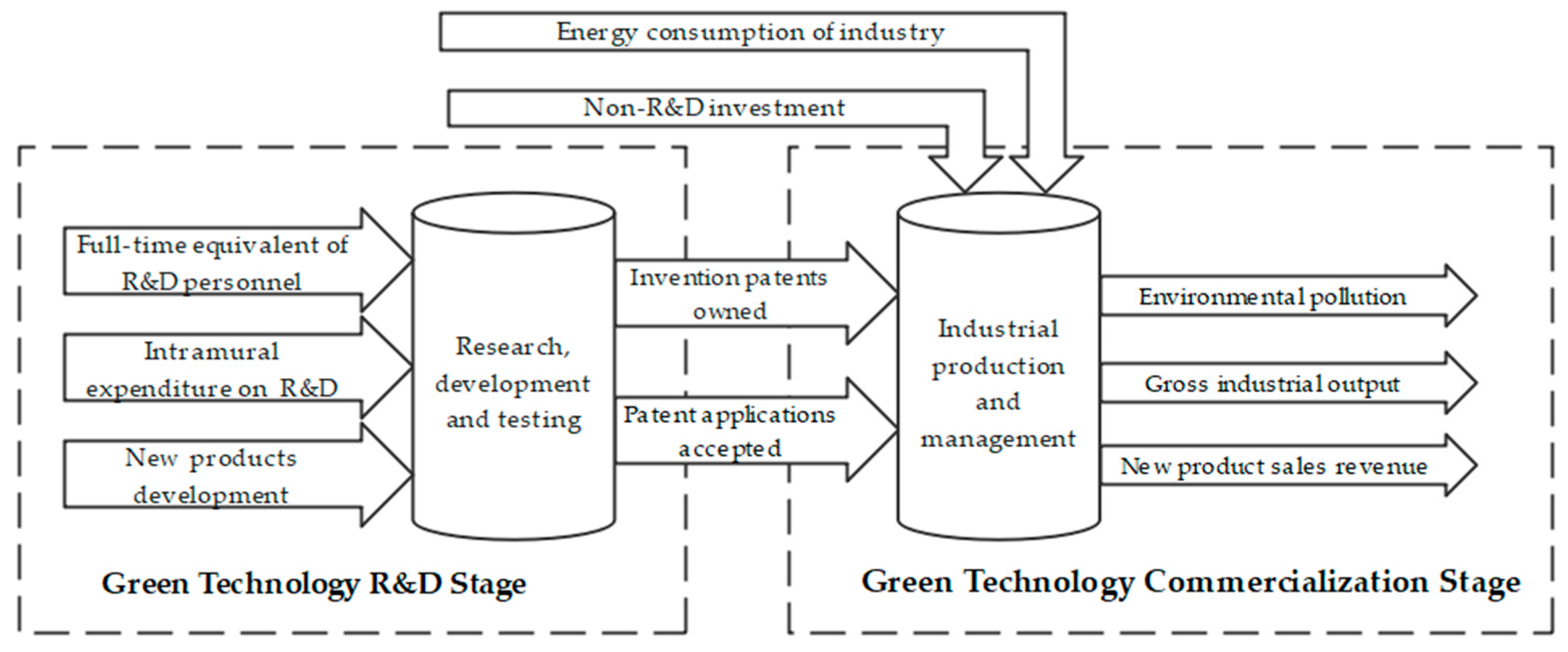
2.1.1. Process of GTI

For the GTI process, adapting from Zhang et al. [9] and Liang and Luo [34], based on the theoretical framework of innovation value chain [23], the transformation of GTI can be divided into two stages: the R&D stage and commercialization stage (see Figure 1).
(1) 
Green technology R&D stage (Stage 1)
During this stage, enterprise R&D is mainly technological innovation achievements oriented, such as gaining patents, requiring massive high-tech human and capital investment. Following expenditure on new product development, intermediate technical outputs such as new technology theories and designs are required to produce the new product. Among the intermediate outputs, patent applications implement the social innovation capability. Compared with utility patents and design patents, invention patents are advanced in technology and its applications are rarely constrained by censorship of the patent licensing agencies, which more objectively reflect the overall strength of regional technological innovation.
(2) 
Green technology commercialization stage (Stage 2)
This stage reflects how industrial enterprises commercialize their R&D achievements for economic benefits. We regard the intermediate outputs from Stage 1 as R&D investments. Non-R&D investment, indicating the cost for acquiring external technology, is the sum of expenditures on foreign technology acquisition, expenditures on domestic technology purchase, expenditures on technology assimilation, and expenditures on technical renovation. Industrial energy consumption is calculated as shown in Section 2.1.2, regarded as the input of the second stage when calculate the efficiency. The comprehensive environmental pollution index is forms through the entropy method for industrial waste water discharges, industrial SO2 emissions, industrial smoke (dust) emissions, total output of industrial solid waste, and industrial CO2 emissions for unit industrial value-added. The calculation of CO2 emissions is presented in Section 2.1.2. The desirable outputs reflect the economic value of the intermediate outputs. Since GTI require intermediate inputs like industrial energy consumption, gross industrial product containing the cost for intermediate inputs is more suitable for this model than the industrial value added [35].
We regard the completion of Stage 1 and the creation of market outputs from Stage 2 marks a routine of successful GTI cycle. Efficiencies of the complete cycle and each stage are measured with DEA and the dynamic and threshold effects are analyzed based on the efficiency scores.
Based on the above analysis and research approach, this study proposes four hypotheses and conducts on such basis.
Hypothesis 1.
The influences of different types of ERs on industrial GTIEs present dynamic effect and lag effect.
Highly linked with the stage-wise transformation process, the characteristics inertia may exist in GTI. It may lead to the dynamic effect and lag effect between ERs and GTIE.
Hypothesis 2.
The nonlinear relationship (threshold effect) exists between different types of ERs and GTIEs.
Different natural and economic conditions such as traffic convenience may influence the relations between ERs and GTIE. And the intensity of various types of ERs may influence the effectiveness among ERs.
Hypothesis 3.
Different types of ERs could have different effects on GTIEs.
The intensity and implementation subjects of types of ER are different. CER is mainly based on laws and regulations, which require mandatory actions to environmental protection and emission reduction of enterprises. MER mostly focuses on charges such as sewages and other wastes. VER has the highest flexibility from the choices of citizens. They may produce different “crowding out effect” and “innovation compensation effect”.
Hypothesis 4.
The impact of ERs on GTIEs has regional differences.
In China, due to the differences in economic development levels, geographical location, resource distribution and environment, energy reserves etc., there are differences in the selection of the intensity and types of ER between different regions [36]. The eastern region has a higher degree of marketization, developed economy and high intensity of environmental regulation. The midland region has apparent geographical characteristics. The ER in northeast and western regions is relatively less and immature. These factors could function towards the effect of ERs on GTIE.

2.1.2. Explained Variables: Industrial Green Technology Innovation Efficiency

Based on the GTI process, we measure GTIE using indicators in Table 1.
Since capital investment (including internal R&D expenditure, expenditure on new product development, and non-R&D investment) influenced both current innovation activities and future innovation activities [37], stock data should replace flow data. The R&D price index is constructed to convert the nominal capital investment into constant price with a base period of 2003. As capital investments mentioned above include labor costs, raw material costs, and fixed asset purchase and construction costs, the R&D price index is constructed by the weighted average of price deflators by the consumer price index, industrial producer price index and fixed asset investment price index is applied. Perpetual inventory method [38] is then used to calculate the stock data as follows:
K i t = E i t + ( 1 δ ) K i t 1
where K i t and K i t 1 are the capital stocks of region i in period t and period t−1; E i t is the real capital investment of region i in period t, transformed from the nominal capital investment by the R&D price index. According to the study of [39], assuming that the growth rate of K is the same as the growth rate of E, the base period capital stock, K 0 , can be written as:
K i 0 = E i 0 g + δ
where g is the average growth rate of E during the period under observation; δ is the depreciation rate set to 15% [37,40].
In addition, to be comparable inter-temporally, we reduce the nominal new product sales revenue and nominal gross industrial product to the constant price in 2003 using the producer price index. Since industrial value added is part of the secondary industry value added, the nominal industrial value added is adjusted to constant prices in 2003 based on secondary industrial value-added index.
Referring to Liang and Luo [34], the innovative transformation time lag is set to two years, that is time spans input for stage 1, output for stage 1, and non-R&D input and output in stage 2 are respectively 2003–2015, 2004–2016 and 2005–2017.

2.1.3. Industrial CO2 Emission

Considering that CO2 takes up nearly 80% of global greenhouse gases and the industrial sector is the main source of material capital production and pollution emissions, industrial energy consumption and industrial CO2 emission are included as environmental factors for calculating industrial GTIE. CO2 emission in this article is consisted of 15 types of energy sources which are raw coal, cleaned coal, other washed coals, coke, coke oven gas, other gases, crude oil, gas oil, kerosene, diesel, oil fuel, liquefied petroleum gases, natural gas, heat, and electricity. Compared with only using the three primary fuels (coal, oil and natural gas) [41], we take all energy sources available including CO2 emission factors, average low calorific value, default carbon content and default carbon oxide factor into consideration to avoid deviations or errors in calculation caused by differences in energy consumption structures across provinces. Referring to the method by IPCC [42], the formula for total industrial CO2 emission is:
( C O 2 ) j = j = 1 15 ( C O 2 ) i j = j = 1 15 E i j × E F i j = j = 1 15 E i j × N C V i j × C E F i j × C O F i j × 44 12
where the subscripts i and j denote provinces and 15 energy sources; E is the industrial energy consumption, collected from the regional energy balance table in China Energy Statistical Yearbook over the years; EF is CO2 emission factors; NCV is the average low calorific value derived from General Rules for Calculation of The Comprehensive Energy Consumption (GB/T 2589-2020); CEF denotes the default carbon content listed in Table 1.4 of 2006 IPCC [42] (COF in newer 2019 edition remain unchanged); COF is the default carbon oxide factor (all set to 1); 44/12 is the gasification coefficient of CO2. Referring to the calculation published by National Development and Reform Commission of China, CO2 emission factor for heat and electricity are 0.6101 tCO2/MWh and 0.11 tCO2/GJ, respectively [43].
For calculating industrial energy consumption E, most current studies use total energy consumption or final energy consumption as proxies [44,45]. However, on the one hand, these two indicators include other industries such as construction; on the other hand, final energy consumption does not fully include industrial energy consumption. Therefore, we apply more detailed calculation. First, all energy transformations are included in calculation as all belong to industrial production. Second, industrial compositions in final energy consumption are included in calculation. Finally, the composition in final energy used as raw materials and materials that do not directly emit CO2 from combustion [46] are removed. And thus, E by industrial CO2 emission is obtained.
For industrial energy consumption deemed as undesired output, the part consumed in industry among final energy consumption of the 15 energy sources and the amount of processing and conversion are converted into “standard coal” and summed. The conversion coefficients for energy sources are provided in GB/T 2589-2020. Industrial energy consumption and industrial CO2 emission can be regarded as two independent variables.

2.1.4. Core Explanatory Variable: Environmental Regulation

ER provides external drives to enterprises for adjusting production methods and reducing environmental pollution. Referring to Zhang et al. and Zhao et al. [9,47], the indicators for the three types of ERs are shown in Table 2.
Among ER-related data, the number of local environmental laws issued in 2011 and 2012 are missing and is replaced with the search results from the legal database of Peking university. To remove the influence of dimensions, ER is obtained by summing three types of ERs, which are respectively obtained by summing normalized indicators.

2.1.5. Control Variables

With existing research and economic implications, the following control variables are incorporated into the model.
(1)
Foreign direct investment (FDI): the proportion of FDI in GDP [48].
(2)
Degree of opening (Open): the ratio of import and export to GDP [49,50]. The import and export are the statistical data divided by location of domestic consumers and producers and is converted into RMB according to annual average exchange rate of USD.
(3)
Industrial structure (Structure): the ratio of the value-added by tertiary industry to GDP [51].
(4)
Enterprise scale (Scale): the ratio of the total product of industrial enterprise above designated size to its number [40,50].
(5)
Degree of intellectual property rights protection (Property): the proportion of technology market turnover in GDP [52].
(6)
Traffic convenience (Traffic): the proportion of length of highways in total area of territory [50].
To be inter-temporal comparable, economic data is adjusted to the constant price in 2003. Regional GDP and technology market turnover are adjusted by the regional GDP Index. The value added by tertiary industry is adjusted by the tertiary industrial value-added index. And the remaining capital data are adjusted by the producer price index. Meanwhile, all control variables are normalized to eliminate the influence of dimension.

2.2. Model Construction

A two-stage network SBM-DEA model is used to evaluate industrial GTIE with MaxDEA 8 Ultra software. Based on the results, efficiency distribution state and dynamic evolution of industrial GTIE in China are further explored by kernel density estimation diagram with RStudio 4.1.1 software. Finally, fixed effect, dynamic effect and threshold effect regressions are used for analyzing the relationship between ERs and GTIE with Stata16.0 software.

2.2.1. Two Stage Network SBM-DEA Model

GTIE is calculated with a non-oriented two-stage network SBM-DEA model [24] under VRS assumption. It is set as n decision making unites (DMUs), D M U j (j = 1, 2, …, n), referring to 29 provinces of China, and each DMU contains k nodes (k = 1, 2). x i j k R + m k , y r j d R + s d and y r j b R + s b respectively represent the inputs of node k, the desired outputs of stage 2 and the undesired outputs of stage 2. The linkage between two nodes is expressed as z p j R + q . s i k , s r d , s r b , s p , s p + represent the slacks of inputs of node k, desired outputs, undesired outputs, intermediate inputs, and intermediate outputs. Hence, the non-oriented two-stage network SBM-DEA model under VRS assumption for D M U 0 is:
ρ 0 = min λ k , s k , s k + w 1 [ 1 1 m 1 ( i = 1 m 1 s i 1 x i 0 1 ) ] + w 2 [ 1 1 m 2 + q ( i = 1 m 2 s i 2 x i 0 2 + p = 1 q s p z p 0 ) ] w 1 [ 1 + 1 q p = 1 q s p + z p 0 ] + w 2 [ 1 + 1 s d + s b ( r = 1 s d s r d y r 0 d + r = 1 s b s r b y r 0 b ) ] s . t .
j = 1 n λ j 1 x i j 1 + s i 1 = x i 0 1 , j = 1 n λ j 2 x i j 2 + s i 2 = x i 0 2 , j = 1 n λ j 2 y r j d s r d = y r 0 d , j = 1 n λ j 2 y r j b + s r b = y r 0 b ,
j = 1 n λ j 1 z p j + s p = z p 0 , j = 1 n λ j 2 z p j s p + = z p 0 , j = 1 n λ j 1 z p j = j = 1 n λ j 2 z p j ,
j = 1 n λ j k = k = 1 2 w k = 1 ,
λ j k 0 , w j k 0 , s i k 0 , s r d 0 , s r b 0 , k = 1 , 2 ,
s p 0 , s p + 0 ,
where ρ 0 is the overall efficiency of D M U 0 ; λ j k is the weight of D M U j in stage k; w k is the weight of sub-process k set at default w 1 = w 2 = 0.5 . “Fixed” link value and “free” link value are two ways to link intermediate variables [24]. Given the context of GTI, this paper uses “free” link value. Based on the optimal slacks of (4), s i 1 , s p + , s i 2 , s p , s r d , s r b , the divisional efficiency of D M U 0 , ρ 0 1 , ρ 0 2 can be measured by the following formula:
ρ 0 1 = 1 1 m 1 i = 1 m 1 s i 1 x i 0 1 1 + 1 q p = 1 q s p + z p 0 ,
ρ 0 2 = 1 1 m 2 + q ( i = 1 m 2 s i 2 x i 0 2 + p = 1 q s p z p 0 ) 1 + 1 s d + s b ( r = 1 s d s r d y r 0 d + r = 1 s b s r b y r 0 b ) ,
where when ρ 0 = 1 , then D M U 0 is overall efficient. When ρ 0 k = 1 , D M U 0 is efficient for node k (k = 1, 2).

2.2.2. Kernel Density Estimation

Kernel density estimation is a non-parametric estimation method that principally fits the sample data through a smooth peak function to describe the distribution of random variables using a continuous density curve. It has the advantage of having strong robustness and weak model dependence and hence is widely applied for research in variable space disequilibrium. The kernel density estimation function takes the form:
f ( x ) = 1 n h i = 1 n K ( x X i h )
where X i represents independent and identically distributed observations which are GTIE of 29 provinces in this article; x is the average; n is the number of observations; h is the bandwidth; K(.) is the kernel function. Gaussian kernel function is used for estimating the kernel density curve. Higher nuclear density curve indicates more counts of provinces at the efficiency level. The changes between kernel density curves in different years indicate the dynamic evolution of industrial GTIEs.

2.2.3. The Benchmark Regression Model

This paper observes the impacts of different types of ERs on industrial GTIEs and analyzes the effects of other factors on GTIEs. Multi col-linearity tests is passed with the maximum VIF coefficient of 4.74, far less than 10. Cluster robust standard error is used for estimation to avoid influence caused by autocorrelation and heteroscedasticity. Because the stage-wise transformation process of GTI exists time lag, GTIE may be influenced by ER in previous years. Since ER lags and lagging duration is uncertain, lags of ER are set as j years (j = 0, 1, 2) (expressions 8 and expressions 9). Considering the possible inertia of GTI, a regression model of GTIE with one year lag (expressions 10 and expressions 11) is established.
G T I E i , t k = α 0 + β E R i , t j + λ j C o n t r o l i , t j + u i + ε i , t ,
G T I E i , t k = α 0 + β 11 C E R i , t j + β 12 M E R i , t j + β 13 V E R i , t j + λ j C o n t r o l i , t j + u i + ε i , t ,
G T I E i , t k = α 0 + α 1 G T I E i , t 1 k + β E R i , t + λ j C o n t r o l i , t j + u i + ε i , t ,
G T I E i , t k = α 0 + α 1 G T I E i , t 1 k + β 11 C E R i , t + β 12 M E R i , t + β 13 V E R i , t + λ j C o n t r o l i , t j + u i + ε i , t ,
where subscripts i and t denote the provinces and year counts; k = 0, 1, 2, are respectively the overall, first, and second stage of industrial GTIE; G T I E i , t 1 k is the GTIE with one year lags; E R i , t j is the ER lagging j years; C E R i , t j , M E R i , t j and V E R i , t j indicate the command-based, market-based, and voluntary ER lagging j years; C o n t r o l i j are control variables, including the FDI, the degree of opening (Open), the industrial structure (Structure), the enterprise scale (Scale), the degree of intellectual property rights protection (Property), and traffic convenience (Traffic); u i represents the fixed effect of provinces; and ε i t is the random disturbance term. If the p-values of E R i , t j , C E R i , t j , M E R i , t j or V E R i , t j , and the p-values of G T I E i , t 1 k are smaller than 0.1, it means that lag effect and dynamic effect exist in the impacts of ERs on GTIEs, respectively.

2.2.4. The Panel Threshold Model

Considering different natural and economic conditions such as traffic convenience may influence the effect of ERs on GTIEs. And the feedback of various types of ERs may be influenced by the intensity of each other. This article takes traffic convenience and various types of ERs as the threshold variables and constructs the following threshold effect model:
G T I E i , t k = α 0 + β 1 E R i , t j I ( t h r e s h o l d i , t γ ) + β 2 E R i , t j I ( t h r e s h o l d i , t > γ ) + λ j C o n t r o l i , t j + u i + ε i , t ,
G T I E i , t k = α 0 + β 11 1 C E R i , t j I ( t h r e s h o l d i , t γ ) + β 11 2 C E R i , t j I ( t h r e s h o l d i , t > γ ) + β 12 M E R i , t j + β 13 V E R i , t j + λ j C o n t r o l i , t j + u i + ε i , t
where threshold represents the threshold variable; I(.) is the indicative function; γ is the threshold value. The threshold effect models with MER or VER as core explanatory variables are like expression (13) which are not explicitly written here. If p-value of self-sampling test is smaller than 0.1 and the estimations between β 1 and β 2 or β 11 1 and β 11 2 are different, it means that threshold effect and nonlinear relationship exists between ERs and GTIEs.

3. Results

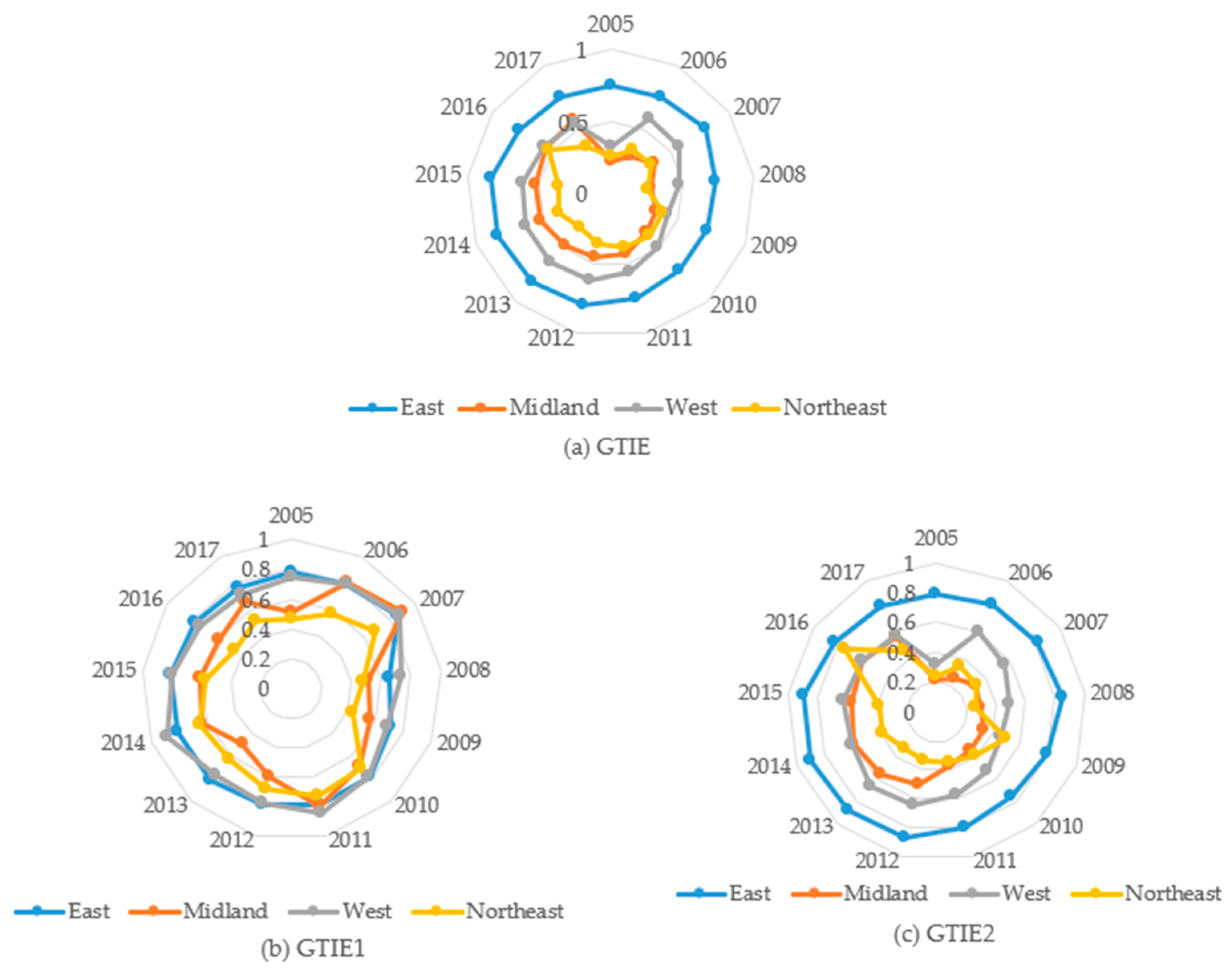
3.1. Results and Analysis of Industrial Green Technology Innovation Efficiency

GTIE of the research objects, 29 provinces of China, is measured through the two-stage network SBM-DEA model. Due to publication, we present the results of 2011 as an example, including industrial GTIE scores and rankings of 29 provinces, with division of 4 regions (according to the division standard of National Bureau of Statistics of China, the eastern region includes 10 provinces: Beijing, Tianjin, Hebei, Shanghai, Jiangsu, Zhejiang, Fujian, Shandong, Guangdong, Hainan; the midland region includes 6 provinces: Shanxi, Anhui, Henan, Hubei, Hunan, Jiangxi; the western region includes 11 provinces: Sichuan, Guizhou, Yunnan, Shaanxi, Gansu, Qinghai, Ningxia, Xinjiang, Chongqing, Guangxi, Neimenggu; the northeastern region includes 3 provinces: Jilin, Liaoning, Heilongjiang [53]. Tibet and Hainan are excluded due to missing data), in Table 3.
It can be found that the average efficiency of GTIE1 is 0.81 and of GTIE2 is only 0.58, indicating that the development of GTI is unbalanced for the two stages. Overall GTIE in most provinces of China are around 0.5, and only a few provinces reach the efficient frontier. Green technology R&D efficiency concentrate around 0.85. Differences between GTIE2 and GTIE seem to be smaller than differences between GTIE1 and GTIE. Also, the average industrial GTIE of the eastern region is around 0.75 while it is only 0.38 in the northeast region, suggesting great regional variances in GTIE.
The kernel density diagram is used to observe the dynamic evolution of industrial GTIEs. The graphical presentations include the overall and stage-wise industrial GTIEs in 2005, 2011 and 2017 (Figure 2).
It can be seen from Figure 2. that, consistent with the tendency from Table 3, overall GTIEs in most provinces of China are still low; green technology R&D efficiency concentrated on a relatively high level; and green technology commercialization has the key influence on overall industrial GTIE increase.
In Figure 2a, overall GTIE distribution present double peak. As the main peak tends to shift right and lowers while side peak gradually elevates, GTIE increased in most provinces and the industrial structure of China is consistently being adjusted and optimized. It also suggests that GTIE is influenced by ERs at a certain extent. Figure 2b presenting single peak leaning to the right. 2005 exhibit a relatively flat curve. As the peak become prominent in 2011 with narrower width, it stretched in 2017. Increasing number of provinces fall back to inefficient state after reaching the efficient frontier, which can be related with the saturation of technology and the increase of R&D difficulty. Regional differences are gradually revealed. In the last figure (Figure 2c), since the side peak is flush with the main peak in 2017, the resources utilization rate in stage 2 has increased rapidly, enabling the convert of technical achievements to correspond economic benefits, however, with severe polarization of the provinces.
Furthermore, considering the great differences in natural resources and the social economic environment in regions, Figure 3 presents the analysis of regional variances of industrial GTIE at the division of the east, midland, west and northeast China.
As presented, during 2005–2017, the overall and stage-wise efficiencies of the midland and the northeast is the lowest and vary significantly to time; the efficiency of the eastern region stably sits the forefront within the country; and while stage 1 is as efficient as the eastern region, other efficiencies of the western region rank the second with clear fluctuation. These can be attributed to the solid economic foundation of the eastern region that creates favorable conditions for R&D and commercialization of industrial green technology, the unbalanced development of the midland region where resources are rich, the improvement of the investment environment and efficient containment of environmental deterioration as the “Western Development” strategy is promoted in the western region, and increasing challenge to resource exhaustion and advanced heavy industry but poor enterprise innovation environment in the northeastern region.
All in all, although overall GTIEs were low in China between 2005 and 2017, it is on the track of steady development. Also, gradient changes can be observed for provinces and regional difference become increasingly prominent.

3.2. Results of Regression

3.2.1. The Test and Empirical Results of the Benchmark Model

The influence and lagging effect of different types of ERs on overall and stage-wise GTIEs are studied further. The results are shown in Table 4. The influence of ERs on the industrial GTIE is not significant under any model with one-year or two-year lag, where Hypothesis 1 does not hold. Hence, we focus on the impact of current ERs on GTIE.
The results of LM test, Hausman test and overidentification test (the traditional Hausman test is not applicable when large difference exists between clustering robust standard error and the ordinary standard error) suggest that the fixed effect model should be applied to regression analysis instead of the mixed regression or random effect model.
Table 4 presents the results that when the explained variables are GTIE and GTIE2, estimation coefficients of ER and MER are significantly positive, but not for VAR. When the explained variable is GTIE1, those of ER and MER are not significant, but the estimation coefficients of VER are negative at the 1% significance level. To note, the estimation coefficients of CER are not significant, suggesting that CER has no influence on both overall and stage-wise GTIEs. This endorses Hypothesis 3 that different types of ERs have different effects on GTIEs. The “innovation compensation effect” of ER on GTIE and GTIE2 is dominant, which can be mainly comes from MER, but VER has may suppress industrial green technology R&D. It can be attributed to the limited binding force of VER overt the enterprises. Budgets are spent on commercial planning for satisfying “environmental protective” sensation of customers. Thus, VER does not truly promote energy savings and emission reduction but puts a “crowding out effect” on green technology R&D. At the same time, as MER in China is yet to mature, most enterprises would rather perform “terminal management” and commercialize present technology than developing new technology to improve the short term economic.
As for control variables, the estimation coefficients of FDI on GTIE, GTIE1 and GTIE2 are respectively positive, not significant and negative. It reflects that effect of FDI is not stable. Concerning scale of enterprises that its estimation coefficients to GTIE and GTIE2 are positive, it is revealed that innovation and commercialization of industrial green technology require scale benefits. With all positive coefficients significant and positive, transportation promotes GTI by supporting the circulation of resources.

3.2.2. The Test and Empirical Results of the Dynamic Effect Model

In this subsection, we further analyze the possible characteristics of inertia of GTI using two-step system GMM. GMM estimation method deals with endogeneity problems that can be caused by explained variables with one-year lag in the dynamic model. System generalized method of moments (system-GMM) overcomes problems such as “weak instrumental variable” for difference GMM [33], reduce potential errors, and correct unobserved individual heterogeneity, missing variable deviation, measurement error and other problems. And two-step system-GMM is generally better than the one-step system-GMM. The results are provided in Table 5.
According to Table 5, the p-value of AR (1) is less than 0.1 and of AR (2) is greater than 0.1, hence, we accept the null hypothesis that the disturbance term has no autocorrelation. With p-value greater than 0.1 except column 4, the null hypothesis cannot be rejected in Hansen tests, so all instrumental variables are effective. Thus, the model setting is justified.
In Table 5, the variable of L.Y represents GTIE, GTIE1 and GTIE2 with one-year lag. As shown, the estimation coefficients of L.Y are significantly positive suggesting that the GTI of industrial enterprises is a yearly continuous process. Hypothesis 1 stands. The explanatory variables are no longer significant in this model, meaning that the removal of inertial influence of GTI results in the equivalence of “innovation compensation effect” of ER and the “crowding out effect”. Only the estimation coefficient of the degree of opening is significant, all positive at least 1% significance level, among the control variables. This indicate that the degree of opening is beneficial to GTIE and FDI is inhibitory to the efficiency of green technology R&D. The dependency on paths for most cities in China explains the observation. It results in focal urban problems including single industrial structure and heavy environmental pollution. Therefore, consequences are different as dynamic factors are introduced. Although ER can encourage enterprises to save energy and reduce emissions, promoting green industrial transformation in Chinese cities takes long time. Import and export trade enables complementing with advantages. But blind introduction of FDI leads to the transfer of some heavy polluting and energy intensive industries in developed countries to the host country, taking up space of green enterprises to survive and hinders industrial enterprises from green technology R&D.

3.2.3. The Test and Empirical Results of the Threshold Effect Model

The nonlinear relationship between different types of ERs and GTIEs is analyzed. Traffic convenience and various types of ERs are selected as threshold variables. The self-sampling test results are that some single threshold tests passed the significance level of 10%, whereas the double threshold fails. Hence, discussion focuses on single threshold model with test and regression results in Table 6 and Table 7.
When the traffic is the threshold variable, all significant threshold values are 0.012 (Table 6). From Table 7, when traffic convenience is extremely poor (traffic ≤ 0.012), the estimation coefficients of ER, CER, VER and MER on GTIE and GTIE2 are significant at 1%, being negative; when the traffic convenience improves (0.012 < traffic), the estimation coefficients is same as the benchmark model (Table 4). Overall, as traffic convenience improves, the influence of various types of ERs on GTIE and GTIE2 overturns from negative to non-influential or positive and the influence of ERs on GTIE1 are not affected. This fully confirms Hypothesis 2 that the threshold effect exists between different types of ERs and GTIEs. The reason is that the level of economic development in areas with extremely inconvenient traffic is poor and the industrial structure is unreasonable. No matter what type of environmental regulation will cause a financial burden on local enterprises, and they lack sufficient resources for green transformation. When the traffic convenience is improved, optimization for allocating resources is more capable, and hence, the “innovation compensation effect” improves rapidly and finally exceeds the “crowding out effect”.
Different types of ERs set to the threshold variable brings different results. First, when ER or VER is the threshold variable, the threshold effect is not significant. Second, when CER is a threshold variable, as CER fastens, the effect of MER on GTIE2 changes from promotion to no effect, and the promotion effect of ER on GTIE2 weakens. This also validates Hypothesis 2. To explain, when degree of CER exceeds the threshold of 0.7593, enterprises invest more funds in pollution control to meet the government legislation and green technology commercialization become less financially supported. Therefore, MER no longer influences GTIE2. Third, when MER is a threshold variable, as MER fastens, the effect of MER on GTIE and GTIE2 changes from negative to positive, and the effect of ER on GTIE2 changes from no effect to promotive. Hypothesis 2 is once more confirmed. As loose MER means fines on pollution is way less than the cost for pollution control, enterprises would prefer paying pollution charges or accept fines. As MER enhances, charges over pollution become more costly where enterprises turn to advancing technology to reduce pollutant emissions, given the target to maximize their own profits. Consequently, green technology commercialization is promoted. Finally, from the above analysis about threshold effects, it can be found that different types of ERs effect GTIE differently, validating Hypothesis 3.
To conclude, regardless of having the threshold variables as CER, MER or traffic convenience, the changes of the impacts of ER and MER over overall and stage-wise industrial GTIEs are consistent, verifying that MER is the main regulatory approach influencing industrial green technology commercialization efficiency. The mutual influences of VER over other types of ER are not clear. The effect of MER is sensitive to the strength of CER, suppressively, but to itself, promotively. The effect of CER is not easy to be affected by other types of ER. Stage 2 of GTI is more sensitive to the nonlinear impact of ERs than stage 1. As CER and MER fasten simultaneously, the enhancement and suppression offset each other so that eventually ER has no nonlinear impact on GTIE. The increase of transportation convenience will promote the positive impact of all types of ERs on industrial GTI.

3.3. Heterogeneity Analysis

The results in 3.1 suggest regional heterogeneity existing in industrial GTIE and hence, we further re-regress using the panel model to explore regional heterogeneity of the influence of ER on GTIE in regions (see regional division in Section 3.1). Combined with LM test, Hausman test, overidentification test and parameter significance test, we use random effect model for regression in the eastern, middle and northeastern regions and use fixed effect model for regression in the western region. Only the model estimation results with significant coefficients are listed here.
(1)
Eastern region
It can be seen from Table 8 that in the eastern region, ER has a positive impact on overall industrial GTIE without lag effect, but no impact on GTIE1 nor GTIE2. The positive effect and lag effect of MER on GTIE and GTIE1 are particularly significant, and MER have a positive one-year lag effect on GTIE2. VER has lag effect on GTIE and GTIE1. CER inhibits the improvement of the GTIE and GTIE2. The results validate Hypothesis 1 and 3. This can be explained that the eastern coastal area has a strong economic base, rich scientific and technological resources, and good market environment. The enterprises hold more advanced ideology for development, and the green innovation is helpful for enterprises to be competitive in the long run. CER breaks the market balance and reduces the benefits of green technology commercialization.
(2)
Midland region
As seen in Table 9, in the midland region, ER has negative impact on overall industrial GTIE and has one-year and two-year lag effect. CER has long-term negative impact on green technology R&D. The current negative impact of MER and VER is apparent with a small number of the effects turning positive along the rise of lag time. Hypothesis 1, 3 are confirmed again. To understand, strong implementation of regulation in the midland region squeezes out R&D funds and increase the operating costs of enterprises in the short run. However, in the long run, enterprises meet ER in more mature measures and greatly reduce the risk of GTI so that the “innovation compensation effect” is gradually greater than the “crowding out effect”.
(3)
Western region
Table 10 shows that in the western region, ER has a positive impact on overall industrial GTIE. The estimated coefficients of CER and MER failed to pass the significance test. VER has positive lag effect on GTIE in each stage, and the long-term lag effect is more obvious than the short-term. Hypothesis 1, 3 are also confirmed in western region. Reasons are that the western provinces actively use regional geographical advantages and rich mineral reserves to vigorously develop tourism and high-tech manufacturing, featuring unique in their economic development. Due to high flexibility of VER, it is more suitable for the western region.
(4)
Northeast region
Table 11 shows that in the northeast region, ER has negative impact on GTIE and lag effect of one-year. The inhibitory effect of VER and MER is obvious, while CER has no significant impact. This results support Hypothesis 1, 3 again. Innovation of the three northeastern provinces greatly improved as the Northeast Revitalization Strategy is applied and the technical standards formulating CER are already met in the industry. Since VER and MER are more flexible, inconsistent treatment measures of VER and MER by enterprises causes scattered effect on technological innovation but increase financial burden for enterprises.
To conclude, the impact of ERs on GTIEs has regional differences, endorsing the Hypothesis 4. Besides, through heterogeneity analysis, Hypothesis 1 and 3 are also confirmed.

4. Discussions and Conclusions

4.1. Discussions

In the measure of GTIE, with the theoretical framework of innovation value chain [23], the time lag between the transformation of the R&D stage and commercialization stage is set to two years. On the one hand, this enriches the application of innovation value chain. On the other, the handle is consistent with previous research result [9,34,54], expanding the relevant research.
ER has a nationwide positive impact on industrial GTIE. ‘Porter hypothesis’ exists in China, which is consistent with existing studies [10,15]. Researchers found that ‘Porter hypothesis’ also holds in European manufacturing sectors, Pakistani manufacturing firms and the Australian oil and gas industry [54,55,56]. However, when the midland and northeastern regions are studied alone, ER has a negative impact. It may be explained by the results from Qiu et al. [57]. Using monopolistic competition model with linear demand and pollution tax, they derived that porter hypothesis holds for more capable firms but fails for the less capable within the same industry [57]. Due to the strong support of the China to the western region and the developed economy in the eastern region, the enterprises in the midland and northeastern regions are relatively less capable. Besides, different types of ERs have differentiated impacts on the GTIE, consistent with [9]. In the analysis of heterogeneity, lag effect is confirmed, consistent with Martínez-Zarzoso et al. in OECD countries, that environmental policy stringency can foster innovation and productivity with one-year and five-year lag [58].
Furthermore, the threshold effect analysis shows that the influences of ERs on the industrial GTIE are affected by the intensity of traffic convenience, VER and MER. This finding enriches the researches of the threshold effect on the relationship between ER and GTIE. The existing studies rarely use traffic awareness as the threshold variable.
Moreover, our results also conclude that inertia features exist in industrial GTI. This finding is in line with the literature pointing to a positive influence of previous innovation experience has on the innovation capacity in European manufacturing sectors [54]. However, the difference is that in China’s industrial sector, after removing the inertial influence of GTIE, ER no longer has an effect. In the European manufacturing sectors, the ER with one-year and two-year lag is still significant [54], indicating that China’s ER needs to be further improved. More detailed comparisons can be done in future research.

4.2. Conclusions

Under the background of Paris Agreement and the United Nations Sustainable Development Goals (SDGs), in this paper, we studied the influences of ER on the industrial GTIE in China from 2005 to 2017. The influences are observed for the overall GTIE and for separate stages. The GTIE of provinces are studied and ranked. Considering the regional features of China, GTIE of regions are also calculated using simple averaged and ranked. The results are analyzed from the perspective of dynamic evolution of GTIE, GTIE1, and GTIE2, also in provinces and regions. Following that, the influences of GTIEs and types of ERs are analyzed with regression. Dynamic effect model and threshold effect models are used for further in-sights. Eventually, as China present typical regional industrial functions, heterogeneity analysis is applied to study GTIEs in eastern, middle, northeastern, and western regions.
The empirical results show that the development of GTI is unbalanced for the two stages. Kernel density diagram indicates that industrial GTIE in China is overall low, with a steadily growing trend. Initial results have been achieved in industrial green transformation. Also, gradient changes can be observed for provinces and its regional difference become increasingly prominent.
Country-wise, ER brings positive influences on GTIE in China, mainly in MER. On the contrary, the VER may cause negative influences on GTIE2. To note, CER has no influence on both overall and stage-wise GTIEs. This is consistent with Hypothesis 3 that different types of ER could have different effects on GTIE. And none of them has the lag effect. To balance the relationship between economy and environment, we need to choose the appropriate type of ER. As for control variables, the effect of FDI on GTIE is not stable, and enterprise scale and traffic convenience are positively related to GTIE.
Considering the stage-wise transformation process of GTI, we further analyze the possible characteristics of inertia of GTI using two-step system GMM. As the dynamic effect model indicates, inertia features exist in GTI, and itis a yearly continuous process. This confirms the prediction of Hypothesis 1, that is, there are dynamic effect in the impact of the ER on GTIE. Although ER can encourage enterprises to save energy and reduce emissions, promoting green industrial transformation in Chinese cities takes long time.
The threshold effect analysis shows that the nonlinear relationship exists between different types of ERs and GTIEs. In other words, their relationship easily be affected by different natural and economic conditions. Which is consistent with Hypothesis 2. In the area with extremely inconvenient traffic, all ERs would bring financial burden on local enterprises that adversely affects GTIEs. When the traffic convenience is improved, the favorable impacts of all ERs on industrial GTI began to prevail. Additionally, the effect of ER and MER is sensitive to the strength of CER, suppressively, but to MER, promotively. The effects of CER and VER are not easily influenced by other types of ERs. Additionally, Stage 2 of GTI is more sensitive to the nonlinear impact of ERs than Stage 1. Therefore, appropriately reducing CER and increasing MER and traffic convenience would improve GTIE, especial GTIE2.
The impact of ERs on GTIE varies regionally, confirming Hypothesis 4. Eastern and western regions are higher in GTIEs both overall and stage-wise. In general, ER positively influence GTIE in eastern and western regions while it presents negative impacts in the midland and northeastern regions. Specifically, in the east, with good market environment and advanced ideology of development, MER and VER promote GTIE and GTIE1 significantly and CER inhibits GTIE2. In the west, provinces actively use regional geographical advantages, featuring unique in their economic development. Hence, VER showing high flexibility is more suitable for promoting GTIEs, but MER and CER could be effectless. In the midland, as accountable measures to ERs mature, the current negative impacts of MER and VER are gradually turning positive as time lags. In the northeast, the inhibitive effects of MER and VER are obvious, while CER has no significant impact. All regions exhibit lag effect in the impacts of types of ERs on overall and stag-wise GTIEs. This is consistent with Hypothesis 1.

4.3. Policy Implementations, Limitations and Future Insights

The section is focused on possible policy implementations and the limitations and prospections to this research.

4.3.1. Policy Implications

Firstly, the Chinese government should, integrating the spatial distribution of GTIE, promote coordinative development across regions and county, and establish a group of energy-saving and environmental protection demonstration zones. It is essential to reduce the excessive reliance over past development pathways for inefficient regions, by promoting cross-regional and cross-national flow of key factors, accelerating the extension of industrial connections, and cultivating competitiveness in new aspects.
Secondly, analysis on the dynamic effect suggest that the government should encourage GTI as the highlight in its long-term strategy. In detail, while optimizing the R&D investment scale and increasing labor for R&D, introducing advanced management experience also increases the financial benefits for enterprises and fundamentally alters mode of “terminal management” for pollution control. Consequently, industrial green transformation can be promoted, shifting globally towards sustainable development directed by the environmental aspect.
Thirdly, international trade should be encouraged to globally popularize green energy-saving products and technology. Also, the threshold study shows that traffic convenience should be enhanced, such as promoting clean energy, intelligent, and digitally advanced transportation equipment. For FDI, especially with on the lower end of global value chain, the government should introduce FDI reasonably to guide foreign investment to high-tech rather than high pollution enterprises. Meanwhile, enterprise scale should be expanded.
Finally, it is necessary to distinguish the impact of three ERs on green technology innovation activities in deferent regions. According to the threshold effect analysis, the government should moderately reduce command-based ER and leverage the market’s leading role, thereby promoting technology innovation upgrade. For example, the government should strengthen the overall connection between trading energy consumption rights and trading carbon emission rights. In eastern regions, command-based ER should be reduced, and market-based and voluntary ER should be strengthened. On the one hand, market mechanism needs perfection; on the other hand, the public should be guided to spontaneously fulfill the responsibility of energy saving and emission reduction. In the central region, the government should reduce current ERs and explore new pathways of ecological lead exploitation and environmental hosting. In the west, market-based ER is in the negative influence range under the threshold, and voluntary ER plays a promoting role. The government build and develop emission trading market and open channels for public environmental supervision. For the northeast regions, reduction to environmental pollution and improvement enterprise innovation should be done through technology support rather than ER. Establishing a comprehensive scientific and technological service system is believed to eliminate lagged production and excessive production capacity, enhance clean and efficient resource use, comprehensively supporting the green transformation of enterprises.

4.3.2. Limitations and Future Insights

Considering progress of updating the China statistical yearbook, the data, especially data of gross industrial output, are only fully updated to 2017 and much data on industrial wastewater discharges is absent after 2017. Concerning the integrity and accessibility of data and the reliability of the conclusions, 2017 is the currently most up-to-date year. The influences of ERs to GTI, especially on GTIE, can be interesting and acutely different as the lifestyles and industrial production structure changes in China under the global pandemic.
However, although dramatic changes are brought by the pandemic, in recent years, the basic process of GTI has not changed significantly, and the transformation of GTI can still be developed in to two stage process, the R&D stage and commercialization stage [59]. Meanwhile, it is recognized that the social and environmental background caused by the epidemic may affect GTI [60], especially the GTI projects started in and after 2019, which requires ER to be more efficient and more conducive to save resources. Comparative calculation can be further made after gaining the complete data.
Additionally, the accuracy of this article can be improved, calling for further efforts. In mechanism, the carbon emission of cement production and different CO2 emission factor for electricity in different regions can be considered into CO2 calculation. In statistics, the significance of estimation coefficients can be influenced by the selection of indicators. Moreover, taking policy as the proxy variable of ER can better deal with the problem of endogeneity.

Author Contributions

Conceptualization, W.S., J.S., Q.M., X.C., W.L. and Y.L.; methodology, J.S. and Q.M.; software, J.S.; validation, J.S.; formal analysis, J.S.; investigation, W.S., J.S. and Q.M.; resources, W.S., X.C. and W.L.; data curation, J.S.; writing—original draft preparation, W.S. and J.S.; writing—review and editing, W.S., J.S. and K.C.; visualization, J.S.; supervision, W.S., X.C. and W.L.; project administration, W.S., X.C. and W.L.; funding acquisition, W.S. and X.C. All authors have read and agreed to the published version of the manuscript.

Funding

This research was funded by the National Natural Science Foundation of China (NSFC), grant number, 11971259 and 12171042, and was funded by the National Social Science Found of China (NSSFC), grant number, 21BTJ072.

Institutional Review Board Statement

Not applicable.

Informed Consent Statement

Not applicable.

Data Availability Statement

The data are not publicly available due to restrictions privacy.

Acknowledgments

This study was sponsored by the National Natural Science Foundation of China (NSFC: 11971259) which is highly acknowledged.

Conflicts of Interest

The authors declare no conflict of interest.

References

  1. Ma, Y.; Zhang, Q.; Yin, Q. Top management team faultlines, green technology innovation and firm financial performance. J. Environ. Manag. 2021, 285, 112095. [Google Scholar] [CrossRef] [PubMed]
  2. National Bureau of Statistics. China Statistical Yearbook on Environment 2006–2020. Available online: https://data.cnki.net/yearbook/Single/N2021070128 (accessed on 24 March 2022).
  3. Zhao, W.D. Reflections and suggestions on industrial green development during the 14th Five-Year Plan. In Proceedings of the China Center for Information Industry Development Industry Economic Forum, Beijing, China, 29 March 2021. [Google Scholar]
  4. China Environmental News. Available online: http://epaper.cenews.com.cn/html/2020-09/30/content_98273.htm (accessed on 24 March 2022).
  5. Zeng, S.; Li, G.; Wu, S.; Dong, Z. The Impact of Green Technology Innovation on Carbon Emissions in the Context of Carbon Neutrality in China: Evidence from Spatial Spillover and Nonlinear Effect Analysis. Int. J. Environ. Res. Public Health 2022, 19, 730. [Google Scholar] [CrossRef] [PubMed]
  6. Wang, H.; Cui, H.; Zhao, Q. Effect of green technology innovation on green total factor productivity in China: Evidence from spatial durbin model analysis. J. Clean. Prod. 2021, 288, 125624. [Google Scholar] [CrossRef]
  7. Liu, D.; Chen, J.; Zhang, N. Political connections and green technology innovations under an environmental regulation. J. Clean. Prod. 2021, 298, 126778. [Google Scholar]
  8. Porter, M.E.; Linde, C.V.D. Toward a New Conception of the Environment-Competitiveness Relationship. J. Econ. Perspect. 1995, 9, 97–118. [Google Scholar] [CrossRef] [Green Version]
  9. Zhang, J.; Ouyang, Y.; Ballesteros-Pérez, P.; Li, H.; Philbin, S.P.; Li, Z.; Skitmore, M. Understanding the impact of environmental regulations on green technology innovation efficiency in the construction industry. Sustain. Cities Soc. 2021, 65, 102647. [Google Scholar] [CrossRef]
  10. Liu, Y.; Wang, A.; Wu, Y. Environmental regulation and green innovation: Evidence from China’s new environmental protection law. J. Clean. Prod. 2021, 297, 126698. [Google Scholar] [CrossRef]
  11. Zhang, P.; Zhang, P.; Cai, G. Comparative Study on Impacts of Different Types of Environmental Regulation on Enterprise Technological Innovation. China Population. Resour. Environ. 2016, 26, 8–13. [Google Scholar]
  12. Zhang, C.; Lu, Y.; Guo, L.; Yu, T. The Intensity of Environmental Regulation and Technological Progress of Production. Econ. Res. J. 2011, 46, 113–124. [Google Scholar]
  13. Li, H.; Zhang, J.; Wang, C.; Wang, Y.; Coffey, V. An evaluation of the impact of environmental regulation on the efficiency of technology innovation using the combined DEA model: A case study of Xi’an, China. Sustain. Cities Soc. 2018, 42, 355–369. [Google Scholar] [CrossRef]
  14. Ye, T.; Zheng, H.; Ge, X.; Yang, K. Pathway of Green Development of Yangtze River Economics Belt from the Perspective of Green Technological Innovation and Environmental Regulation. Int. J. Environ. Res. Public Health 2021, 18, 10471. [Google Scholar] [CrossRef] [PubMed]
  15. Zhao, T.; Zhou, H.; Jiang, J.; Yan, W. Impact of Green Finance and Environmental Regulations on the Green Innovation Efficiency in China. Sustainability 2022, 14, 3206. [Google Scholar] [CrossRef]
  16. Wu, F.; Fu, X.; Zhang, T.; Wu, D.; Sindakis, S. Examining Whether Government Environmental Regulation Promotes Green Innovation Efficiency—Evidence from China’s Yangtze River Economic Belt. Sustainability 2022, 14, 1827. [Google Scholar] [CrossRef]
  17. Wang, F.; Jiang, T.; Guo, X. Government quality, environmental regulation and green technological innovation of enterprises. Sci. Res. Manag. 2018, 39, 26–33. [Google Scholar]
  18. Bai, J.; Jiang, K.; Li, J. Using Stochastic Frontier Model to Estimate the Efficiency of Regional R&D and Innovation in China. Manag. World 2009, 10, 51–61. [Google Scholar]
  19. Yang, G. Reviews of Returns to Scale in DEA models. Chin. J. Manag. Sci. 2015, 23, 64–71. [Google Scholar]
  20. Charnes, A.; Cooper, W.W.; Rhodes, E. Measuring the efficiency of decision making units. Eur. J. Oper. Res. 1978, 2, 429–444. [Google Scholar] [CrossRef]
  21. Kao, C. Efficiency decomposition in network data envelopment analysis: A relational model. Eur. J. Oper. Res. 2009, 192, 949–962. [Google Scholar] [CrossRef]
  22. Fan, J.; Xiao, Z.H. Analysis of spatial correlation network of China’s green innovation. J. Clean. Prod. 2021, 299, 126815. [Google Scholar] [CrossRef]
  23. Hansen, M.T.; Birkinshaw, J. The Innovation Value Chain. Harv. Bus. Rev. 2007, 85, 121–130, 142. [Google Scholar]
  24. Tone, K.; Tsutsui, M. Network DEA: A slacks-based measure approach. Eur. J. Oper. Res. 2009, 197, 243–252. [Google Scholar] [CrossRef] [Green Version]
  25. National Bureau of Statistics. China Statistical Yearbook 2004–2018. Available online: http://www.stats.gov.cn/tjsj/ndsj/ (accessed on 24 March 2022).
  26. National Bureau of Statistics. China Industrial Economy Statistical Yearbook 2006–2018. Available online: https://data.cnki.net/Yearbook/Single/N2021020054 (accessed on 24 March 2022).
  27. Editorial Board of China Environment Yearbook. China Environment Yearbook 2006–2018. Available online: https://data.cnki.net/yearbook/Single/N2021070108 (accessed on 24 March 2022).
  28. National Bureau of Statistics; Ministry of Science and Technology of the People’s Republic of China. China Statistical Yearbook of Science and Technology 2004–2018. Available online: https://data.cnki.net/yearbook/Single/N2022010277 (accessed on 24 March 2022).
  29. National Bureau of Statistics. China Energy Statistical Yearbook 2006–2018. Available online: https://data.cnki.net/yearbook/Single/N2021050066 (accessed on 24 March 2022).
  30. EPS Database. Available online: https://www.epsnet.com.cn/index.html#/Index (accessed on 24 March 2022).
  31. Macrochina Statistical Database. Available online: http://edu.macrochina.com.cn/skins/11/stat/index.shtml?ny=1 (accessed on 24 March 2022).
  32. The Official Website of National Bureau of Statistics of China. Available online: https://data.stats.gov.cn/easyquery.htm?cn=E0103 (accessed on 24 March 2022).
  33. BeiJing Statistical Yearbook 2018. Available online: http://nj.tjj.beijing.gov.cn/nj/main/2018-tjnj/zk/indexch.htm (accessed on 24 March 2022).
  34. Liang, S.; Luo, L. The Dynamic Effect of International R&D Capital Technology Spillovers on the Efficiency of Green Technology innovation. Sci. Res. Manag. 2019, 40, 21–29. [Google Scholar]
  35. Chen, S. Green Industrial Revolution in China: A Perspective from the Change of Environmental Total Factor Productivity. Econ. Res. J. 2010, 45, 21–34. [Google Scholar]
  36. Peng, X.; Li, B. On Green Industrial Transformation in China under Different Types of Environmental Regulation. J. Financ. Econ. 2016, 42, 134–144. [Google Scholar]
  37. Griliches, Z. R&D and Productivity Slowdown. Am. Econ. Rev. 1980, 70, 343–348. [Google Scholar]
  38. Goldsmith, R.W. A Perpetual Inventory of National Wealth. Stud. Income Wealth 1951, 14, 5–74. [Google Scholar]
  39. Goto, A.; Suzuki, K. R&D capital, rate of return on R&D investment and spillover of R & D in Japanese manufacturing industries. Rev. Econ. Stat. 1989, 71, 555–564. [Google Scholar]
  40. Li, Q.; Wang, W.; Xiao, R. Research on the regional disparities of China’s industrial enterprises green innovation efficiency from the perspective of shared inputs. China Popul. Resour. Environ. 2018, 28, 27–39. [Google Scholar]
  41. Chen, S. Energy Consumption, CO2 Emission and Sustainable Development in Chinese Industry. Econ. Res. J. 2009, 44, 41–55. [Google Scholar]
  42. National Greenhouse Gas Inventories Programme; Eggleston, H.S.; Buendia, L.; Miwa, K.; Ngara, T.; Tanabe, K. 2006 IPCC Guidelines for National Greenhouse Gas Inventories; IGES: Hayama, Japan, 2006. [Google Scholar]
  43. National Development and Reform Commission of China. The Notice of Reporting and Verifying Annual Carbon Emissions and Making Plans of Emission Monitoring from the General Office of National Development and Reform Commission of China. Available online: https://www.ndrc.gov.cn/xxgk/zcfb/tz/201712/t20171215_962618.html?code=&state=123 (accessed on 24 March 2022).
  44. Yang, S. Evaluation and Prediction on Carbon Emissions Transferring across the Industrial Sectors in China. China Ind. Econ. 2015, 327, 55–67. [Google Scholar]
  45. He, X.; Zhang, Y. Influence Factors and Environmental Kuznets Curve Relink Effect of Chinese Industry’s Carbon Dioxide Emission—Empirical Research Based on STIRPAT Model with Industrial Dynamic Panel Data. China Ind. Econ. 2012, 1, 26–35. [Google Scholar]
  46. Liu, Z.; Geng, Y.; Xue, B.; Xi, F.; Jiao, J. A Calculation Method of CO2 Emission from Urban Energy Consumption. Resour. Sci. 2011, 33, 1325–1330. [Google Scholar]
  47. Zhao, L.; Gao, H.; Xiao, Q. An Empirical Study of Environment Regulation Influence on Efficiency of Green Technology Innovation. Stat. Decis. 2021, 37, 125–129. [Google Scholar]
  48. Jing, W.; Zhang, L. Environment Regulation, Economic Opening and China’s Industrial Green Technology Progress. Econ. Res. J. 2014, 49, 34–47. [Google Scholar]
  49. Nie, M.; Qi, H. Can OFDI Improve China’s Industrial Green Innovation Efficiency?: Based on the Perspective of Innovation Value Chain and Spatial Correlation Effect. Word Econ. Stud. 2019, 2, 111–122. [Google Scholar]
  50. Xiao, Q.; Lu, Z. Heterogeneous Environment Regulation, FDI and the Efficiency of China’s Green Technology Innovation. Mod. Econ. Res. 2020, 4, 29–40. [Google Scholar]
  51. Jiang, Z.; Lyu, P. Stimulate or inhibit? Multiple environmental regulations and pollution-intensive Industries’ Transfer in China. J. Clean. Prod. 2021, 328, 129528. [Google Scholar] [CrossRef]
  52. Hu, K.; Wu, Q.; Hu, Y. The Effects of Intellectual Property Rights Protection on Technology Innovation: Empirical Analysis Based on Technology Trading Market and Provincial Panel Data in China. J. Financ. Econ. 2012, 38, 15–25. [Google Scholar]
  53. National Bureau of Statistics of China. From January to October 2021, the national investment in real estate development increased by 7.2%. Available online: http://www.stats.gov.cn/xxgk/sjfb/zxfb2020/202111/t20211115_1824507.html (accessed on 24 March 2022).
  54. Rubashkina, Y.; Galeotti, M.; Verdolini, E. Environmental regulation and competitiveness: Empirical evidence on the Porter Hypothesis from European manufacturing sectors. Energy Policy 2015, 83, 288–300. [Google Scholar] [CrossRef] [Green Version]
  55. Javeed, S.A.; Latief, R.; Jiang, T.; Ong, T.S.; Tang, Y.J. How environmental regulations and corporate social responsibility affect the firm innovation with the moderating role of Chief executive officer (CEO) power and ownership concentration? J. Clean. Prod. 2021, 308, 127212. [Google Scholar] [CrossRef]
  56. Ford, J.A.; Steen, J.; Verreynne, M.L. How environmental regulations affect innovation in the Australian oil and gas industry: Going beyond the Porter Hypothesis. J. Clean. Prod. 2014, 84, 204–213. [Google Scholar] [CrossRef] [Green Version]
  57. Qiu, D.; Zhou, M.; Xu, W. Regulation, innovation, and firm selection: The porter hypothesis under monopolistic competition. J. Environ. Econ. Manag. 2018, 92, 638–658. [Google Scholar] [CrossRef]
  58. Martínez-Zarzoso, I.; Bengochea-Morancho, A.; Morales-Lage, R. Does environmental policy stringency foster innovation and productivity in OECD countries? Energy Policy 2019, 134, 110982. [Google Scholar] [CrossRef] [Green Version]
  59. Gao, H.G.; Xiao, T. Whether the heterogeneous environmental regulation can force the optimization of industrial structure—Based on the mediating effect and threshold effect of industrial green technology innovation efficiency. Jianghan Trib. 2022, 3, 13–21. [Google Scholar]
  60. Habibi, Z.; Habibi, H.; Mohammadi, M.A. The Potential Impact of COVID-19 on the Chinese GDP, Trade, and Economy. Economies 2022, 10, 73. [Google Scholar] [CrossRef]
Figure 1. Green technology innovation process.
Sustainability 14 04717 g001
Figure 2. 2005–2017 China’s industrial GTIE kernel density diagram and dynamic evolution.
Sustainability 14 04717 g002
Figure 3. 2005–2017 Regional differences and evolution trend of China’s industrial GTIE.
Sustainability 14 04717 g003
Table 1. Explained variables.
VariableExplanationsIndicators
Industrial GTIEGreen technology R&D stage
(Stage 1)
Input variables
(2003–2015)
R&D investmentFull-time equivalent of R&D personnel
Internal R&D expenditure
Expenditure on new product development
Output variables
(2004–2016)
Intermediate outputsDomestic invention patents owned
Domestic patent applications accepted
Green technology commercialization stage
(Stage 2)
Input variables
(2005–2017)
R&D investmentIntermediate outputs
Non-R&D investmentSum of expenditure
Output variables (2005–2017)Desirable outputSales Revenue of New Products
Gross industrial output
Undesirable outputEnergy consumption of industry for unit industrial value-added
The environmental pollution index
Table 2. Explanatory variables.
VariableExplanationsIndicators
ERCommand-based ERTotal number of local environmental laws, regulations, and standards issued
The number of environmental administrative punishment cases
Market-based ERInvestment in treatment of industrial pollution sources
Receipt from of fee on wastes discharge
Environmental protection investment in environmental protection acceptance projects
Voluntary ERNumber of environmental proposals by the NPC * and CPPCC *
Number of environmental petitions completed
* NPC stands for national people’s congress. * CPPCC is National Committee of the Chinese People’s Political Consultative Conference.
Table 3. Industrial GTIE and rankings of 29 provinces in 2011.
RegionGTIERankingGTIE1Ranking1GTIE2Ranking2
Nation0.577 0.810 0.575
East0.75410.79630.7961
Midland0.42830.79820.3753
West0.56720.85010.5672
Northeast0.38440.72940.3424
Beijing0.84850.6962411
Tianjin0.597130.708220.59413
Hebei0.368230.776190.27125
Shanxi0.218270.809170.16629
Neimenggu0.209280.521280.22427
Liaoning0.296260.480290.25626
Jilin0.665110.92870.59812
HeilongJiang0.191290.780180.17228
Shanghai0.77880.5562711
Jiangsu111111
Zhejiang0.680100.89490.64011
Anhui0.437200.765200.30224
Fujian0.83170.6622611
Jiangxi0.474170.810160.51615
Shandong0.68690.867120.66110
Henan0.420210.698230.43217
Hubei0.467180.820150.42118
Hunan0.551150.886110.41519
Guangdong111111
Guangxi0.530160.97650.44416
Chongqing0.599120.90980.57414
Sichuan0.394220.865130.32021
Guizhou0.319250.95460.31022
Yunnan0.83260.6642511
Shanxi0.333240.836140.30723
Gansu0.575140.736210.6639
Qinghai111111
Ningxia0.442190.891100.393320
Xinjiang111111
Note: Tibet and Hainan are excluded.
Table 4. Results of the benchmark model.
VariablesGTIEGTIE1GTIE2
(1)(2)(3)(4)(5)(6)
ER0.0361 * −0.0340 0.0545 **
(1.76) (−1.37) (2.12)
CER −0.0126 0.0034 −0.0211
(−0.41) (0.10) (−0.53)
VER −0.0265 −0.1417 ** 0.0076
(−0.37) (−2.22) (0.09)
MER 0.1067 * −0.0022 0.1334 **
(1.91) (−0.05) (2.09)
Open−0.1758−0.2394−0.0202−0.1381−0.2921−0.3364
(−0.95)(−1.29)(−0.10)(−0.71)(−1.22)(−1.44)
FDI0.2817 ***0.2326 ***−0.0018−0.0043−0.3322 ***−0.2678 **
(−3.12)(−2.77)(−0.01)(−0.03)(−3.00)(−2.50)
Structure0.06060.0565−0.2171−0.20090.18680.1765
(0.46)(0.42)(−1.57)(−1.45)(1.22)(1.12)
Scale0.2412 **0.2213 **−0.0188−0.05220.2955 *0.2812
(2.29)(2.06)(−0.16)(−0.45)(1.75)(1.68)
Property−0.03770.02700.26870.2427−0.1753−0.0832
(−0.16)(0.12)(0.90)(0.83)(−0.44)(−0.22)
Traffic0.4461 ***0.3947 ***0.2754 **0.2989 **0.5059 ***0.4336 ***
(4.70)(3.68)(2.32)(2.38)(4.58)(3.44)
Constant0.3367 ***0.3543 ***0.7246 ***0.7549 ***0.3039 ***0.3180 ***
(5.94)(6.19)(12.40)(13.54)(4.38)(5.20)
Observations377377377377377377
LM[0.0000][0.0000][0.0000][0.0000][0.0000][0.0000]
Hausman[0.0100][0.0071][0.0923][0.0696][0.0024][0.0018]
Overid[0.0000][0.0000][0.0079][0.0001][0.0000][0.0000]
Note: ***, ** and * represent significant levels of 10%, 5% and 1%; the t value is in (); the p value of the corresponding statistics is in [].
Table 5. Results of the dynamic effect model.
VariablesGTIEGTIE1GTIE2
(1)(2)(3)(4)(5)(6)
L. Y0.3902 ***0.3957 ***0.3299 ***0.3289 ***0.3089 **0.2833 *
(2.97)(2.72)(3.36)(2.70)(2.40)(1.77)
ER−0.0435 0.0102 −0.0348
(−0.81) (0.21) (−0.89)
CER −0.0559 0.0733 −0.0382
(−0.58) (0.72) (−0.34)
VER −0.2634 0.0094 −0.1421
(−1.11) (0.04) (−0.95)
MER 0.0603 −0.0367 0.0516
(0.44) (−0.20) (0.50)
Open0.4536 **0.4038 **0.2193 *0.2210 *0.5877 ***0.5878 ***
(2.55)(2.31)(1.79)(1.70)(4.62)(3.70)
FDI−0.1254−0.1083−0.2694 **−0.2959 **−0.0040−0.0325
(−1.04)(−0.87)(−2.31)(−2.00)(−0.03)(−0.22)
Structure−0.01620.05680.13460.1342−0.0966−0.0534
(−0.13)(0.42)(0.84)(0.83)(−0.69)(−0.38)
Scale0.12210.0196−0.00280.00290.06950.0126
(0.92)(0.15)(−0.02)(0.01)(0.47)(0.08)
Property0.14940.12850.11630.07470.3033 **0.3158 *
(0.95)(0.72)(0.77)(0.39)(2.19)(1.86)
Traffic−0.03510.0499−0.1830−0.1531−0.1609−0.1396
(−0.23)(0.25)(−1.40)(−1.06)(−0.89)(−0.64)
Constant0.3073 ***0.3072 ***0.5021 ***0.5059 ***0.4134 ***0.4093 ***
(3.46)(3.15)(4.90)(4.13)(3.89)(3.43)
Observations348348348348348348
AR (1)[0.016][0.020][0.001][0.002][0.020][0.021]
AR (2)[0.145][0.247][0.449][0.487][0.429][0.365]
Hansen[0.289][0.272][0.128][0.043][0.572][0.556]
Note: ***, ** and * represent significant levels of 10%, 5% and 1%; the t value is in (); the p value of the corresponding statistics is in [].
Table 6. Test results of threshold effect.
Explained VariablesExplanatory VariablesThreshold QuantityThreshold ValueF-Statisticp-ValueBS Times
Threshold variable: Traffic
GTIEERSingle0.01231.110.03300
CERSingle0.01228.050.03300
MERSingle0.01232.370.05300
VERSingle0.01227.820.05300
GTIE2CERSingle0.01221.690.08300
MERSingle0.01225.080.09300
VERSingle0.01221.40.09300
Threshold variable: CER
GTIE1MERSingle0.159612.030.07300
GTIE2ERSingle0.759315.380.05300
MERSingle0.759313.780.08300
Threshold variable: MER
GTIEMERSingle0.179417.770.07300
GTIE2ERSingle0.433419.290.06300
MERSingle0.179415.630.09300
VERSingle0.430821.730.06300
Note: only shows the test results passing the significance level of 10% is presented in table.
Table 7. Results of the threshold effect model.
Panel A: Results of the Threshold Effect Model with Traffic as the Threshold Variable
VariablesGTIE GTIE2
Core ExplanatoryVariables (X)ERCERMERVERCERMERVER
(1)(2)(3)(4)(6)(7)(8)
VER(CER)(CER) −0.0226−0.0120−0.01170.0117−0.0204−0.0202
(−0.32)(−0.40)(−0.38)(0.14)(−0.52)(−0.51)
MER(VER)(MER) 0.0931 *−0.02220.0930 *0.1194 *0.01210.1192 *
(1.81)(−0.31)(1.81)(1.99)(0.15)(1.99)
X × I (Traffic ≤ γ)−1.1018 ***−3.4437 ***−3.9486 ***−2.6035 ***−3.5725 ***−4.0726 ***−2.6525 ***
(−9.98)(−5.87)(−28.44)(−5.89)(−5.74)(−24.83)(−5.54)
X × I (γ < Traffic)0.0312−0.01120.0917 *−0.0223−0.01970.1178 *0.0119
(1.56)(−0.37)(1.79)(−0.31)(−0.50)(1.97)(0.15)
Control variablesYesYesYesYesYesYesYes
Observations377377377377377377377
Panel B: Results of the Threshold Effect Model with CER or MER as the Threshold Variable
VariablesThreshold: CERThreshold: MER
Explained VariablesGTIE1GTIE2GTIEGTIE2
Core Explanatory Variables (X)MERERMERMERERMERVER
(1)(2)(3)(4)(5)(6)(7)
VER(CER)(CER)0.0672 * 0.0784−0.0102 −0.0184−0.0150
(1.93) (1.48)(−0.33) (−0.46)(−0.38)
MER(VER)(MER)−0.1199 * 0.0192−0.0258 0.00840.0954
(−1.99) (0.26)(−0.36) (0.10)(1.67)
X × I (Threshold ≤ γ)0.08310.1117 ***0.1710 **−1.1817 *−0.0517−1.2813 **−0.2276
(1.68)(2.97)(2.42)(−2.00)(−1.32)(−2.11)(−1.63)
X × I (γ < Threshold)−0.04240.0590 **0.05330.0950 *0.0556 **0.1205 *0.0831
(−0.98)(2.29)(0.85)(1.83)(2.21)(2.01)(0.97)
Control variablesYesYesYesYesYesYesYes
Observations377377377377377377377
Note: ***, ** and * represent significant levels of 10%, 5% and 1%; the t value is in (); the p value of the corresponding statistics is in [].
Table 8. Results in the eastern region.
VariablesGTIEGTIE1 GTIE2
(1)(2)(3)(4)(5)(6)
No Lag
ER0.0460 * 0.0334 0.0421
(1.94) (1.56) (1.28)
CER −0.0826 0.0756 −0.1620 *
(−1.30) (1.21) (−1.81)
MER 0.1395 ** 0.1347 ** 0.1017
(2.11) (2.00) (1.44)
One-year lag
LCER −0.1225 *0.03290.0159 −0.1754 **
(−1.71)(1.34)(0.15) (−2.36)
LVER 0.1287 ** 0.1216 * 0.1066
(2.03) (1.75) (1.05)
LMER 0.1449 *** 0.1236 ** 0.1086 **
(3.49) (2.10) (2.02)
Two-year lag
L2MER 0.1044 ** 0.1744 *** 0.0199
(2.05) (2.68) (0.36)
Note: ***, ** and * represent significant levels of 10%, 5% and 1%; the t value is in (); the p value of the corresponding statistics is in [].
Table 9. Results in the midland region.
VariablesGTIEGTIE1GTIE2
(1)(2)(3)(4)(5)(6)
No Lag
ER−0.0939 * −0.0924 ** −0.0976
(−1.85) (−2.16) (−1.13)
VER 0.1442 −0.4000 *** 0.2664
(0.88) (−4.10) (1.19)
MER −0.1462 *** −0.1072 *** −0.1645 *
(−2.76) (−3.16) (−1.67)
One-year lag
LER−0.0929 ** 0.0512 −0.1180
(−2.10) (1.4140) (−1.49)
LVER 0.2681 0.1907 * 0.3624
(1.10) (1.83) (1.19)
LMER −0.1245 ** 0.0266 −0.1635 *
(−2.46) (0.34) (−1.84)
Two-year lag
L2ER−0.1064 ** 0.0208 −0.1428 **
(−2.44) (0.5579) (−2.16)
L2CER −0.0234 −0.0942 *** 0.0253
(−0.27) (−2.63) (0.25)
L2VER 0.3618 * 0.3753 0.4091
(1.73) (1.25) (1.47)
L2MER −0.1127 0.1293 *** −0.1949
(−1.34) (3.21) (−1.43)
Note: ***, ** and * represent significant levels of 10%, 5% and 1%; the t value is in (); the p value of the corresponding statistics is in [].
Table 10. Results in the western region.
VariablesGTIEGTIE1GTIE2
(1)(2)(3)(4)(5)(6)
No Lag
ER0.0868 * 0.0058 0.0904
(1.82) (0.10) (1.58)
One-year lag
LVER 0.0942 0.2949 ** 0.0344
(0.88) (2.49) (0.32)
Two-year lag
L2VER 0.3111 ** 0.3576 *** 0.2559 **
(2.74) (4.20) (2.31)
Note: ***, ** and * represent significant levels of 10%, 5% and 1%; the t value is in (); the p value of the corresponding statistics is in [].
Table 11. Results in the northeast region.
VariablesGTIEGTIE1GTIE2GTIE2
(1)(2)(3)(4)(5)(6)
No Lag
ER−0.0506 *** −0.1147 −0.1147
(−3.07) (−1.56) (−1.56)
VER −0.5349 ** −0.7028 ** −0.7028 **
(−1.98) (−2.14) (−2.14)
MER −0.0192 −0.2633 *** −0.2633 ***
(−0.50) (−11.13) (−11.13)
One-year lag
LER−0.0598 * −0.1053 ** −0.0684
(−1.6788) (−2.07) (−1.06)
LVER −0.1090 ** −0.6144 *** 0.0873
(−2.44) (−16.10) (1.48)
LMER −0.1564 *** −0.2039 ** −0.1569 ***
(−11.36) (−1.96) (−2.72)
Two-year lag
L2MER −0.2223 *** −0.1483 *** −0.2637 ***
(−23.03) (−3.12) (−5.40)
Note: ***, ** and * represent significant levels of 10%, 5% and 1%; the t value is in (); the p value of the corresponding statistics is in [].
Publisher’s Note: MDPI stays neutral with regard to jurisdictional claims in published maps and institutional affiliations.

