Hydrological Modeling of Aquifer’s Recharge and Discharge Potential by Coupling WetSpass and MODFLOW for the Chaj Doab, Pakistan

Abstract

The estimation of the groundwater (GW) potential in irrigated areas is crucial for the sustainable management of water resources in order to ensure its sustainable use. This study was conducted in a selected area of the Chaj doab, Punjab, Pakistan, to quantify the impacts of the pumping and the recharge on the aquifer therein. To that end, a groundwater flow model (MODFLOW) and a groundwater recharge model (WetSpass) were coupled to assess the conditions of the aquifer. The model was calibrated manually on twelve-year data (2003–2014) against the observed groundwater levels, and it was validated with five-year data (2015–2019). Three main scenarios (divided into ten subscenarios) were simulated for the future prediction of the groundwater: Scenario-I (to assess the impact of the pumping if the prevailing conditions of the years from 2003 to 2019 were to continue until 2035); Scenario-II (to assess the impact of the pumping on the aquifer by increasing the pumping capacity by 25, 50, 75, and 100% for the coming 10 years); and Scenario-III (to assess the impact on the aquifer of the decrease in the average groundwater recharge from the river by 50% by following the same pumping trend). The Scenario-I results show that there would be an 18.1 m decrease in the groundwater table at the end of the year 2035. The Scenario-II results predict decreases in the water table by 2.0, 5.5, 9.8, and 14.3 m in the year 2029 as a result of increases in the pumping capacity of 25, 50, 75, and 100%, respectively. The results of Scenario-III show that, with the decrease in the recharge from the rainfall, there would be a 0.7 m decrease in the water table, and that, from open-water bodies, there would be a 2.4 m decrease in the water table. These results are very helpful for determining the recharge and discharge potential of the aquifer.

1. Introduction

Water availability is essential for meeting agricultural, domestic, and industrial needs. In the past few decades, the burden on the groundwater resources of Pakistan has increased because of their unchecked, unguided, and unregulated exploitation [1]. At a global level, about 750–800 billion cubic meters (BCM) of groundwater is being consumed for agriculture [2,3]. Shortfalls in the surface water is the reason for the increasing use of groundwater [4]. The supply of surface water has decreased significantly in recent years, and the demand for groundwater has also increased proportionately [5]. Groundwater resource management in the Chaj doab, Pakistan, and especially in the Khadir canal subdivision, is necessary for improving agriculture and protecting the ecosystem, as well as for biodiversity [6].

The high exploitation of the groundwater in the Chaj doab is putting the aquifer’s future at risk [7]. Currently, more than 1.2 million tube wells are operating in the country and, among these, 86% are operating in Punjab [3]. Agricultural areas are turning into barren lands because of the reduced availability of groundwater. A total of 15% of the agricultural area has been turned into barren lands because of the decrease in the water table at a rate of 2 to 3 m per year [8]. This over pumping of the groundwater is because of the exponential increase in agricultural and industrial demands to fulfill the supply–demand gap. The task of the management of the groundwater resources in the area of the Khadir canal subdivision can be achieved with the help of an integrated groundwater model, which requires input in the form of the recharge and other parameters.

Various numerical methods have been developed to address the limitations of analytical solutions and to deal with the complexity of groundwater systems. Several numerical methods in groundwater studies are available: the finite element method (FEM); the finite difference method (FDM); the finite volume method (FVM); and the boundary element method (BEM). Groundwater models are simplified versions of real systems [9], and they have been applied for groundwater resource management under different scenarios [10,11,12,13,14,15,16,17,18,19]. The interaction between the groundwater and the surface water is important for management [20,21,22,23,24,25]. Among all of the models, MODFLOW is the most widely used groundwater flow model [26,27]. The WetSpass model has been used for the groundwater recharge and for evapotranspiration estimation [28]. A good coupling of WetSpass and MODFLOW was achieved in order to understand the characteristics of groundwater [29,30]. The WetSpass model was coupled with MODFLOW to evaluate the groundwater replenishment efficiency of the natural reservoirs in the floodplain of the Drava River, Hungary [31].

The integration of the surface water and groundwater models was necessary in order to find probable solutions for the local and global groundwater management problems for aquifer sustainability. Major areas of Pakistan are falling under scarcity of groundwater. The Chaj doab is an area in Pakistan that lies between two major converging rivers: the Chenab and Jhelum Rivers. The doab has faced a significant decrease in the groundwater level over the last three decades. Many researchers have studied the groundwater in different areas other than the Chaj doab by using MODFLOW, as the groundwater recharge is a major parameter; however, in all of the previous studies, the modelers have taken a lumped value of the recharge from the rainfall. This study aims to estimate the groundwater level and flow, and the predictions for its future under different scenarios. In this study, the groundwater recharge model, WetSpass, was coupled with the groundwater flow model, MODFLOW-2005. Future scenarios were developed according to the possible phenomena that may occur because of climate change or management perspectives. These scenarios are helpful for the generation of guidelines for saving the groundwater resources in the investigated area.

2. Materials and Methods

2.1. Study Area

The area of Khadir, which is a canal subdivision that is situated in the Chaj doab (the region between the Chenab and Jhelum Rivers), Punjab, Pakistan, has an overall landmass of 1139 km². The Lower Jhelum Canal (LJC) irrigates the Punjab Province, which is located between the longitudes, 72°30′ and 73°15′ east, and the latitudes, 31°36′ and 32°15′ north, as is indicated in Figure 1.

There is a gentle slope of 0.3 m/km, and an elevation range of 155–255 m throughout the majority of the region. During the months of June through October, the west monsoon is chiefly responsible for the region’s significant rainfall. The region receives 65 to 70 percent of its total rainfall in the monsoon season, which ranges from roughly 1000 mm towards the northeast, to 230 mm towards the southwest of Punjab [32].

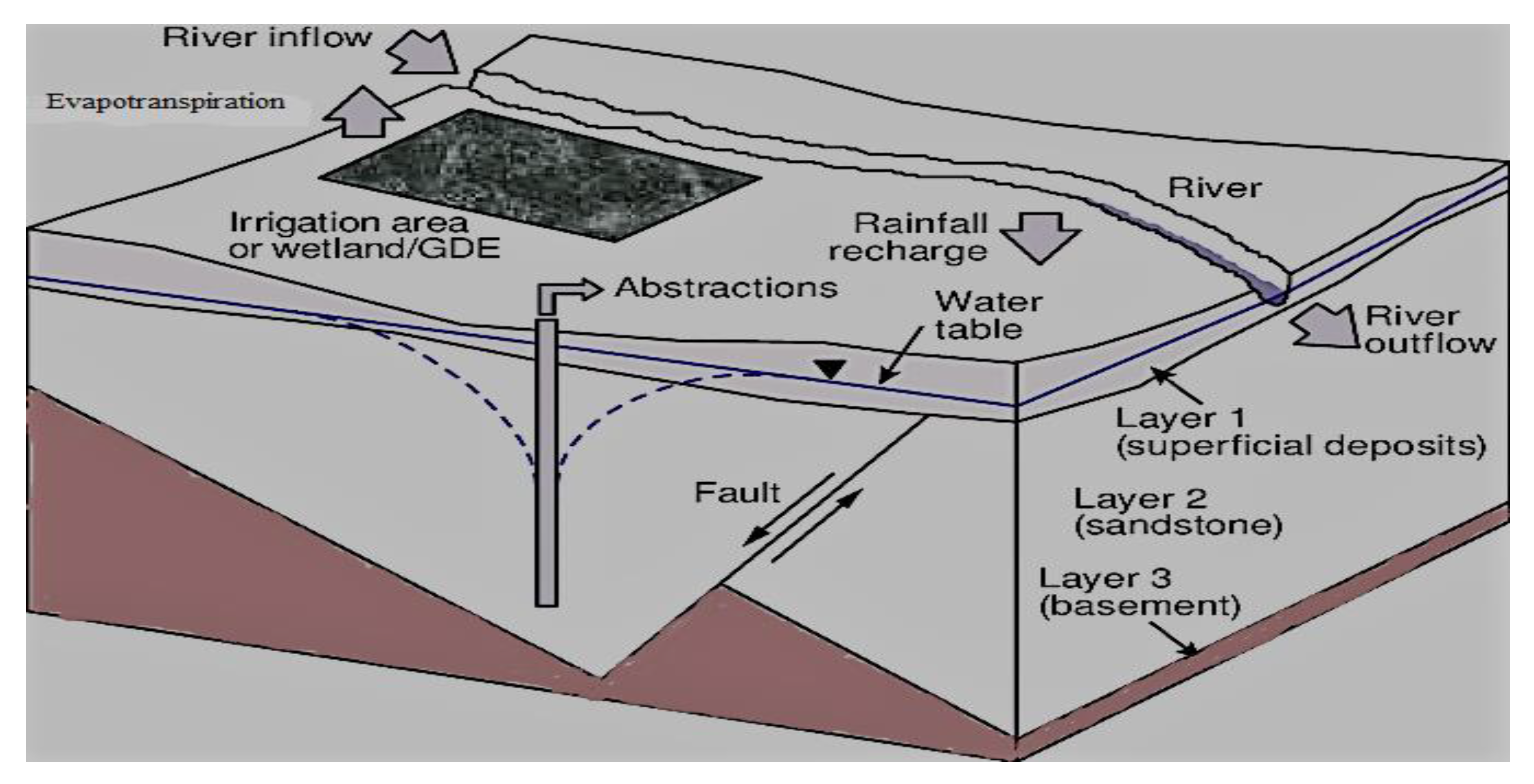
2.1.1. Conceptual Modeling Approach

The formulation of a conceptual model is a very crucial step for the development of the numerical model for the purpose of a modeling study. The intention of the conceptual model development is helpful for the simplification of the actual model. A successful conceptual model should be very close to the actual field conditions of the system. It is difficult to study actual systems because of the large number of complexities, and so the conceptual model is very important for the simulation of the actual field conditions. A good conceptual model carries less chances of errors in the numerical models. The designed conceptual model is based on the initial conditions of the model, the boundary condition, the layers, the starting and end times, the digital elevation of the model/study area layout, the climatic parameters (i.e., rain, ET, sunshine hours, wind speed), the recharge, the discharge, the groundwater level, and the grid size. However, on the basis of the provided initial conditions, the conceptual model is converted into the numerical model by applying the values of all of the parameters in the numerical model, “MODFLOW”. A pictorial elaboration of the conceptual model is shown in Figure 2.

2.1.2. Climatic Data

The input data of the climatic parameters for the WetSpass-M were taken from the Pakistan Meteorological Department from 2000 to 2019. The minimum and maximum long-term annual rainfalls were 424 and 679.5 mm, respectively, with a mean value of 455.7 mm. A notable fluctuation in the long-term temperature was observed in the summer (April–September), with a temperature range between 19 and 41 °C, and, in the winter season (October–March), with a range between 4 and 28 °C. The long-term monthly wind speed data show that the maximum wind speed was recorded on July 9 at 674 km/h, and that the minimum wind speed was 1.02 km/h.

2.1.3. Lithology

The lithological data for the study area were obtained from the Water and Power Development Authority (WAPDA). A comprehensive study was conducted by the Water and Soil Investigation Division [33] to determine the subsurface lithology and the geological characteristics of the Chaj doab, Pakistan. Only sixteen boreholes (Figure 1d) in the study area were found. The sampling depths of the data, on average, were taken at 20 cm. The sampling results show that the lithology was comprised of fine (silty clay, clay, and sandy clay) and moderately fine soil (clay loam, sandy clay loam, and silty clay loam), as is shown in (Figure 1c).

2.1.4. Topography

A map of the topography of the study area was attained from the Shuttle Radar Topography Mission (STRM-1), with a 30 m resolution, and by using the link: https://earthexplorer.usgs.gov/ (accessed on 24 October 2020). The elevation ranged between 155 and 255 m at the lowest and highest points, with an average elevation of 190 m from the mean sea level (Figure 1b).

2.2. Groundwater Data

The groundwater level data were collected from 19 piezometers from the Punjab Irrigation Department, the “Sargodha Irrigation Zone”, for the period from 2003 to 2019. The groundwater level data were collected two times yearly: one time during the premonsoon (June), and the second time during the postmonsoon (October), and these data were available. The mean groundwater depth fluctuation in the area for the period from 2003 to 2019 was recorded as 5.32 m, as is shown in Figure 3.

2.3. Groundwater Recharge and Evapotranspiration

The spatial scattering of the evapotranspiration and the groundwater recharge was taken from [34]. The WetSpass-M [35] is widely applied to evaluate the distribution of the groundwater balance component model on a spatial basis [35,36,37,38,39,40]. The WetSpass-M model takes the spatial distributions of the soil, the slope, the groundwater depth, the land use, and the climatic data. The seasonal water balance distribution was considered to be:

P = S + ET + R

(1)

P stands for precipitation; S is used to indicate the surface runoff; ET is for evapotranspiration; and R denotes the groundwater recharge. The runoff, recharge, interception, and evapotranspiration are all included in the WetSpass-M ArcGIS integrated model as input parameters. The weather/climatic data (potential evapotranspiration, temperature, wind speed, and rainfall), the terrain, the soil texture, the land use/land cover, the leaf-area index data, and the groundwater depth are all basic inputs for this model. It also takes into account a number of other variables [14,28]. ArcGIS was used to prepare all of the input data, which were then imported into the model with the same cell size in ascii format. To prepare the input data from 2000 to 2019, ArcGIS 10.3.1 was used, and the raster cell size was maintained at 100 m × 100 m. Each parameter has a total of 72,713 grids. WetSpass is based upon the principle of the water balance. As a result, the average annual recharge from the rainfall was between 99.10 and 177.2 mm, with a mean value of 119.4 mm per year, as is displayed in (Figure 4a). The long-term annual evapotranspiration values for the years from 2000 to 2019 ranged between 134.4 and 287.2 mm/year, with a mean value of 231 mm/year, as is depicted in (Figure 4b).

2.4. Groundwater Flow Model Setup

A fully distributed three-dimensional groundwater flow model, MODFLOW-2005 [41], was developed with the help of ModelMuse [42] as a graphical user interface. The partial differential equation that was used in MODFLOW for the groundwater flow is from [43]:

$$\frac{\partial }{\partial \mathrm{x}}\left[{\mathrm{K}}_{\mathrm{xx}}\frac{\partial \mathrm{h}}{\partial \mathrm{x}}\right]+\frac{\partial }{\partial \mathrm{y}}\left[{\mathrm{K}}_{\mathrm{yy}}\frac{\partial \mathrm{h}}{\partial \mathrm{y}}\right]+\frac{\partial }{\partial \mathrm{z}}\left[{\mathrm{K}}_{\mathrm{zz}}\frac{\partial \mathrm{h}}{\partial \mathrm{z}}\right]\pm W_f={\mathrm{S}}_{\mathrm{s}}\frac{\partial \mathrm{h}}{\partial \mathrm{t}}$$

(2)

where x, y, and z are the three-dimensional major axes of the hydraulic conductivity coordinates along the K_xx, K_yy, and K_zz [LT⁻¹]; h is the head, which is known to be potentiometric [L]; W_f is the volumetric flux with the per unit volume on behalf of the sinks of water and/or resources, where the extractions are denoted with negative values, and the injections [T⁻¹] are denoted with positive values; S_s denotes the porous-material-specific storage [L⁻¹]; and t is time [T].

The groundwater flow system (aquifer) contained three layers, according to the geological boreholes and pumping tests (first: 0–8 m; second: 8–40 m; and third: 40–107 m), with each layer having a thickness of 8, 32, and 67 m, respectively. In this study, the aquifer layers were defined on the basis of the lithology [32]. According to the lithology of the aquifer model, Layer-1 was defined as “unconfined”, Layer-2 was defined as “unconfined to convertible”, and Layer-3 of the third aquifer was defined as “confined”. To make sure, the precision of the model grid was discretized by 100 m by 100 m, subsequent in a purview of 113 rows and 643 columns and having a total of 72,713 cell numbers, and three layers calculated by the WetSpass model. In boundary conditions, the average groundwater level over twenty years was assigned as the initial hydraulic head. The eastern boundary was taken at Chenab River (Stream-1), and it was assigned river packages to simulate the recharge and river stage impacts at the aquifer. The northern boundary, which is represented by the escape canal (Stream-2), was also assigned river packages. All of the other channels in the study area were also assigned river packages. The western and southern boundary was assigned as a general head boundary on the basis of the records of the observation wells, as is shown in (Figure 5). Well packages (WEL) (used in MODFLOW to simulate the GW flux) were applied to the pumping wells, and recharge packages (RCH) (used to simulate the recharge at the top of the model in MODFLOW) were applied to the groundwater data.

The hydraulic properties were defined on the basis of the available bore log data. These included the horizontal and vertical hydraulic conductivities, as well as the aquifer storage properties. The hydraulic conductivity that was given to the model varied between 1 and 119 m/day as the maximum and minimum values, respectively, with an average value of 66 m/day. A similar hydraulic conductivity range within the province of the Punjab realm was used by the authors of [44,45,46]. Only 5% of Layer-1 had a horizontal hydraulic conductivity (HHC) value in the range of 1–30 m/day, 80% had an HHC value in the range of 30–80 m/day, and the remaining 15% had an HHC value in the range of 80–108 m/day, as is shown in (Figure 6a). From the spatial distributions of the HHCs for Layer-2 and Layer-3, it was found that only 3% of Layer-2 and Layer-3 had an HHC value in the range of 1–30 m/day, 80% had an HHC value in the range of 30–80 m/day, and 17% had an HHC value in the range of 80–119 m/day, as is shown in (Figure 6b).

The vertical hydraulic conductivity of Layer-1 was 1 ≤ over 75% of the total area, with 5% in a range of 1–1.5 m/day, and the remaining 20% in a range of 1.5–2 m/day. For the distribution of the spatial vertical hydraulic conductivities for Layer-2 and Layer-3, it was found that 45% of the aquifer was in the range of 0–3 m/day, 35% percent was in the range of 3–4 m/day, and 20% was in the range of 5–6 m/day. The specific yield (Sy) ranged between 0.05 and 0.25 as the minimum and maximum values, respectively. The average daily recharge ranged between 0.000271 and 0.000597 m/day as the minimum and maximum values, respectively, with an average value of 0.000387 mm/day.

2.5. Coupling of Surface Water Model and Groundwater Flow Model

Because of its lumped nature, the WetSpass model is essentially restricted in terms of dealing with the groundwater flow. MODFLOW, on the other hand, has problems identifying the distributed evapotranspiration and the groundwater recharge, which are the primary inputs to the groundwater model. As a result, it appears that, if WetSpass-based evapotranspiration and groundwater recharge are used as the input data in MODFLOW, and the groundwater level is estimated and transferred to WetSpass, the spatiotemporal characteristics of the study region will be adequately represented. The coupled WetSpass–MODFLOW framework in this study integrated calibrated hydrological modeling (WetSpass-M) with a calibrated groundwater flow model (MODFLOW), as is illustrated in Figure 7. WetSpass simulates the water balance components. MODFLOW, on the other hand, models the three-dimensional groundwater flow and its related sources and sinks (e.g., recharge, discharge to drains, interaction with lakes, and interaction with stream networks). The outputs of the WetSpass-M model were utilized as the inputs to MODFLOW. MODFLOW calculates the groundwater hydraulic head and the groundwater-surface water interactions, which are then fed into WetSpass. A coupled model of this type was used to analyze the current stage and the future conditions of the hydrology (water balance components, system water budget, and groundwater level) of the Khadir canal subdivision.

2.6. Calibration, Validation, and Sensitivity Analyses

Average long-term parameters, such as the average value of the precipitation, the PET mean, the mean level of the groundwater, and the mean values of the groundwater recharge, were used to create the steady-state model as a starting step for the transient-state model. A total of 19 average observation-well groundwater levels were used to calibrate the steady-state model. The value, R² = 0.98, was found to be a significant fit between the simulated and observed heads. The root mean square error was 0.0022 m, while the mean error was −0.018 m. The mean absolute error was 0.51 m. The steady-state model was used as an initial condition for the transient model; however, the mismatch between the transient- and steady-state models’ starting points in 2003 proved useless.

Data from 2003 to 2007 were utilized for the warm-up period of the transient model, while data from 2008 to 2014 were used for the model calibration. The transient model outcomes are depicted in Figure 8a, compared to a time series of the observation well heads. This hydrograph depicts the mean values of the observed and simulated water table heads for a transient-stage model (Figure 8c). For the calibration of the groundwater head, 19 observation wells were used over a period of 12 years to record the groundwater levels. The value of R² was found to be 0.99, and it is a significant fit between the simulated and observed heads. Calibrated groundwater model parameters are shown in

Table 1. Parameters of the calibrated groundwater model.

Parameter	Value	Unit	Description
HKZ1	550	m d−1	Zone 1: Hydraulic conductivity
HKZ2	60	m d−1	Zone 2: Hydraulic conductivity
HKZ3	52.17	m d−1	Zone 3: Hydraulic conductivity
HKZ4	44.04	m d−1	Zone 4: Hydraulic conductivity
RCH	0.95 R	mm d−1	Groundwater recharge
Q	1	mm d−1	Discharge rate
EVT	1.1 ET	mm d−1	Evapotranspiration
RIVC1	30	m2 d−1	Conductance of River Stream-1
RIVC2	30	m2 d−1	Conductance of River Stream-2
GHB	10	m2 d−1	General head boundary conductance

R denotes GW recharge, and ET represents evapotranspiration.

. The mean errors ranged from 0.10 to 0.32 m, and the root mean square error was 0.0027 min total.

Table 2. Statistical analysis of field and model data.

Parameter	Formula	Values
		Calibration	Validation
Mean Error	$\mathrm{ME}=\frac{1}{n}{{\displaystyle \sum }}_{i=1}^n\left(H_{obs}-H_{sim}\right)$	–0.01836	0.102705
Mean Absolute Error	$\mathrm{MAE}=\frac{1}{n}{{\displaystyle \sum }}_{i=1}^n\left|H_{obs}-H_{sim}\right|$	0.5158	0.3162
Root Mean Square Error	$\mathrm{RMSE}=\sqrt{\frac{1}{n}{{\displaystyle \sum }}_{i=1}^n(H_{obs}-H_{sim}{)}_i^2}.$	0.0022	0.0027
R2		0.98	0.99

shows the statistical analysis. Data from 2015 to 2019 were used for the model validation, as is shown in (Figure 8b).

A sensitivity analysis was performed by using the computer program known as UCODE (universal sensitivity analysis, calibration, and uncertainty evaluation) [47], and by using ModelMate [48]. The program was used for studying the sensitivity of the hydraulic conductivity (HKZ), the groundwater recharge (RCH), the discharge (Q), the evapotranspiration (EVT), the general head boundary (GHB), and the river conductance (RIVC). The parameters of the discharge (Q), the recharge (RCH), and the hydraulic conductivity (HKZ4) were found to be more sensitive, and the parameters of the hydraulic conductivity (HKZ2) and the general head boundary represent the least sensitive parameters. Moreover, the pumping rate (Q) and the groundwater recharge were found to be highly sensitive groundwater model parameters, as is shown in (Figure 9).

3. Results

3.1. Groundwater Flow Model Budget

The groundwater budget at the transient-state condition of the calibrated MODFLOW model at the last time step is displayed in

Table 3. Groundwater budget at transient-state condition.

Parameter	Inflow		Outflow		Inflow—Outflow
	m3 day−1	%	m3 day−1	%	m3 day−1
GHB Boundary	653,060.9	29.45	74,174.36	3.35	578,886.5
River	1,216,020	54.84	154,223.5	6.96	1,061,797
Recharge	348,247.3	15.71	0	0	348,247.3
Evapotranspiration	0	0	53,563.36	2.42	−53,563.36
Wells	0	0	1,935,358	87.28	−1,935,358
Total	2,217,329	100	2,217,329	100	0

. The results show that the inflow from the river seepage was 1,216,020.25 m³ d⁻¹, and that it contributed 54.84% of the total inflow (2,217,328.50 m³ d⁻¹) to the aquifer. The seepage from the general head boundary represented 29.45% of the total inflow to the aquifer. The groundwater recharge contributed 15.71% to the inflow to the aquifer. The outflow quantification of the aquifer showed that 87.28% (1,935,357.59 m³ d⁻¹) of the total outflow was due to the pumping of the wells from the aquifer, and that the remaining 3.35% of the outflow represented the general head boundary (GBH), with 6.96% due to river recharge, and 2.24% due to evapotranspiration.

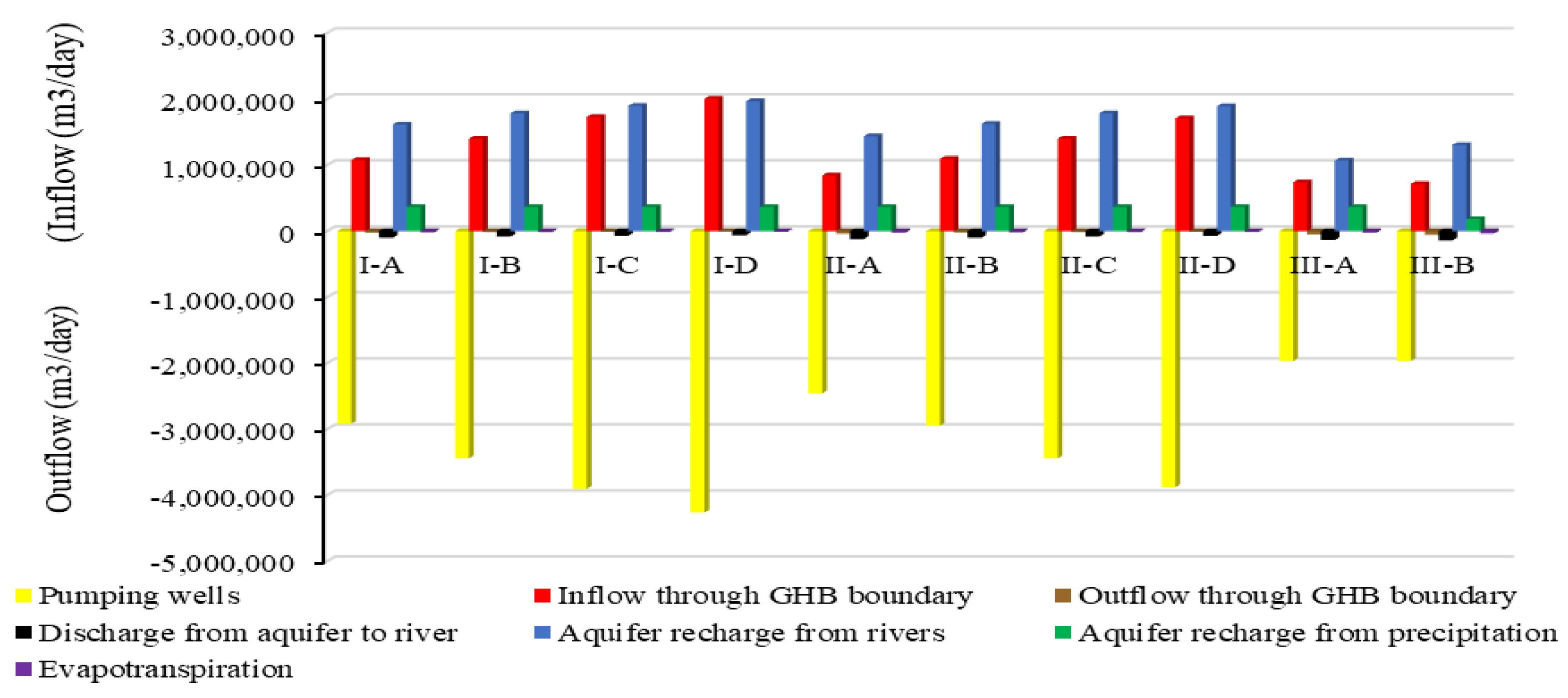
3.2. Simulated Scenarios

3.2.1. Scenarios

The calibrated model was run for different scenarios of the investigated area. These scenarios were developed on the basis of possible situations that may cause a shortage of water resources that may stress the aquifer in the coming days. The developing scenarios are helpful for the development of proper measures and management strategies to counter future problems.

Scenario-I was simulated to assess the impact of pumping if the prevailing conditions of the years from 2003 to 2019 were to continue until 2035, as there are no regulations to control the extensive tube well installation in that area. The scenario was further subdivided into I-A, I-B, I-C, and I-D, according to the simulation times of 2020, 2025, 2030, and 2035, respectively. In this scenario trend of increasing pumping, the volume was also analyzed, as a massive increase in tube wells in the study area was observed. Scenario-II was used to simulate the impacts of pumping on the aquifer by increasing the pumping capacity by 25, 50, 75, and 100% for the coming 10 years. This means that, in this scenario, the aquifer status was analyzed on the basis of increasing the pumping rate with the aforementioned percentages over a period of ten years. It was further subdivided into the scenarios, II-A, II-B, II-C, and II-D, according to the increase in the pumping capacity. Scenario-III was subdivided into the subscenarios, III-A and III-B, under the conditions that were simulated by decreasing, on average, the groundwater recharge from the rainfall by 50%, and from the river by 50%, following the same pumping that is shown in

Table 4. Summary of simulated scenarios.

Scenarios		Pumping Wells	Inflow Through GHB Boundary	Outflow Through GHB Boundary	Discharge from Aquifer to River	Aquifer Recharge from Rivers	Aquifer Recharge from Precipitation	Evapotranspiration	Groundwater Level
		×104 m3/day							M
	Reference	−194.98	64.41	−6.8	−15.37	120.99	36.49	−4.79	0
I	I-A	−291.5	107.63	−2.26	−10.01	161.38	36.49	−1.74	−5
	I-B	−344.13	140.1	−1.33	−8.23	178.41	36.49	−1.31	−9.8
	I-C	−390.46	173	−0.83	−6.99	189.81	36.49	−1.01	−14.6
	I-D	−426.26	200.67	−0.56	−6.24	196.75	36.49	−0.85	−18.1
II	II-A	−245.88	84.28	−4.02	−12.16	143.72	36.49	−2.43	−2
	II-B	−294.79	109.52	−2.19	−9.89	162.56	36.49	−1.71	−5.3
	II-C	−344.02	140.03	−1.33	−8.24	178.38	36.49	−1.33	−9.8
	II-D	−387.66	170.87	−0.86	−7.06	189.24	36.49	−1.03	−14.3
III	III-A	−196.69	73.95	−4.94	−13.42	106.9	36.49	−2.29	−2.4
	III-B	−196.72	71.52	−5.63	−14.15	130.43	18.24	−3.69	−0.7

.

In this study, three main scenarios (which were divided into ten subscenarios) were simulated for the future prediction of the groundwater. A summary of these scenarios is depicted in Table 4.

The results of Scenario I-A show that there was a 5.0 m decrease in the groundwater table in 2020 from the reference point of the calibrated steady-state model (2000–2019), with a pumping rate of 2,915,029 m³/day. In the 1-B scenario, the model predicted that the groundwater table would decrease by up to 9.8 m in the year 2025, which is due to the pumping rate of 3,441,109 m³/day from the level. For Scenario I-C, the groundwater was predicted to decline by 14.6 m from the reference because of the increase in the pumping rate to 3,904,630 m³/day in 2030, and Scenario I-D simulated a decrease of 18.1 m in the year 2035, and the pumping rate was predicted to be 4,262,693 m³/day in 2035, as is shown in Table 4. The simulated results of Scenario II-A show that, by increasing the discharge from pumping by 25%, the groundwater table would decrease by up to 2.0 m by the end of 2029, from the reference. The Scenario II-B results show a decrease of 5.5 m at 50% increased pumping. The Scenario II-C results show a decrease of 9.8 m at 75% increased pumping, and the Scenario II-D results show a decrease of 14.3 m at 100% increased pumping in the year 2029, from the reference. The Scenario III-A results predicted that, by decreasing the recharge from the river and other water bodies by 50%, because of uncertain climate change, drought, etc., the aquifer recharge from the river was 1,069,024 m³/day instead of 2,134,048 m³/day in 2019, which caused a 2.4 m decrease in the water table from the reference. The Scenario III-B results predicted that, by decreasing the recharge from the rainfall by 50%, because of uncertain climate change, drought, etc., the aquifer recharge from the rainfall was 182,482 m³/day instead of 364,890 m³/day in 2019, which caused a 0.7 m decrease in the water table from the reference. A graphical representation of the recharge to, and the discharge from, the aquifer under different scenarios is shown in (Figure 10).

Because of the imbalance between the groundwater abstraction and the recharge at different locations, many mixed drawdown levels were seen at every observation well. It was simulated that, at most of the locations, there was lowering in the water table, and at only very few observation wells, there was lowering in the groundwater level. The model predicted that the groundwater level in the vicinity of the monitoring in Pir Panja, and towards the riverside of the Khadir distributary, would be little affected by the discharge until 2035. Similarly predicted results show that the groundwater levels in the observation wells in the vicinity of Vijhalke Minor, Kalri Minor, and Walla Minor were decreasing less than the observation wells that were installed near Khadir Minor. For Scenario-I, the contour intervals of the groundwater table were kept constant for each year. The ranges of the minimum and maximum contour lines of the groundwater table varied from 159 to 189 m, and from 138 to 186 m, for the years 2020 and 2035, respectively, as is shown in Figure 11a,b, respectively.

For Scenario-II (A, B, C, D), the ranges of the minimum and maximum groundwater table values varied at 165–189, 159–189, 147–189, and 141–189 m at 25, 50, 75, and 100% increases in the pumping rate, respectively. For Scenario-III (A, B), the ranges of the minimum and maximum groundwater table values varied from 165–192 m and 166–190 m at a 50% decrease in the recharge from the rainfall and river, respectively, as is shown in (Figure 12a,b).

In the higher side of the study area, a substantial drawdown was observed, while, on the lower side, or riverside, of the study area, there was less of a decrease in the water table until 2035. The greater decrease in the upper side was due to less recharge from the river, as it lies away from the river. This lowering in the groundwater level in the future may cause a very drastic situation for crop production as well as for domestic and industrial uses. Decreases in the groundwater level may have drastic impacts on pumping, such as an increase in the pumping cost, and a decrease in the pumping efficiency. The results of a study that was based on the groundwater economy, which was conducted by the authors of [4] in the Indus basin, Pakistan, show that the decline in the groundwater table could have significant impacts on the pumping cost. A shallow electronic turbine (operating < 6 m) could cost up to USD 1000, while a deep electronic turbine/tube well (operating > 20 m) could cost up to USD 5000 per annum. Similarly, the pumping cost of deep tube wells was also more (i.e., USD 8.61 per acre inch, compared to USD 18.78 for a 31 and 91 m lift in the water [49]).

For sustainable management, and for aquifer replenishment, the groundwater recharge from rainfall must be increased through the promotion of rainwater harvesting in order to assess the continuous decrease of using it for groundwater recharge. In areas that are suffering a continuous decrease in the groundwater table, the techniques of artificial recharge must be applied by using the rainfall water and extra surface irrigation water for the groundwater replenishment. There should be the formation and implementation of legal boundaries to evaluate the unjudicial abstraction, and the unnecessary use of the groundwater. This study may be extended to the regional scale by incorporating further management and climate change scenarios.

3.2.2. Model Uncertainty

The current model produces a good interaction between the surface water and the groundwater for the proper management of groundwater resources. The data required a comprehensive quantitative analysis for their uncertainty. Most of the major uncertainties in the model are due to the available data constraints, such as the measured groundwater levels and observation wells, as well as poor meteorological, soil, physical, and hydraulic data availability. Recording the river’s recharge over time and a comparison of the historical data with the forecasts for current and future conditions, as well as the refinement of the groundwater recharge, would help the model to become more accurate in terms of the short-term future uncertainty. Using the current conceptual model as a starting point, it will be possible to refine the model and reduce its uncertainty as the network for monitoring the groundwater levels increases.

4. Conclusions

The management of groundwater supplies is critical to the achievement of agricultural, domestic, and industrial growth. The future potential of the Chaj doab aquifer in Punjab, Pakistan, was studied by using a distributive surface water model, which is known as WetSpass, and a groundwater flow model, which is known as MODFLOW. With twelve years of data (2003–2014), and five years of validation data, the groundwater flow model, MODFLOW, was calibrated and validated manually (2015–2019). The R² was found to be 0.99, which is an acceptable fit between the simulated and observed heads. In this work, three primary scenarios (which were separated into ten subscenarios) were simulated for the future groundwater predictions, and the root mean square error was 0.0027 m. The predicted results of Scenario-I indicate that the groundwater in the study area may decrease from 1.5 to 18.1 m over a period of 16 years (2019–2035). A greater decrease was observed in the area where the tube well density was high. Similarly, a smaller decrease in the groundwater table (from normal to medium) was simulated in the lower part of the study area of concern.

In Scenario-II, the results were simulated by increasing the pumping rate by 25, 50, 75, and 100% over 10 years (2020–2029). The results predict that, after 10 years, the groundwater table would decrease by up to 2.0, 5.3, 9.8, and 14.3 m through the increases in the pumping rate of 25, 50, 75, and 100%, respectively. The Scenario-III results reveal that, with the decreases in the groundwater recharge from the rainfall and the river by 50% due to climate change or to a decrease in the river recharge, the mean decreases in the water table would be 0.7 m and 2.4 m, respectively. A greater decrease in the water table through the decrease in the groundwater table was recorded by the river recharge, compared to the recharge from the rainfall. On the higher side of the study area, a substantial drawdown was observed, while, on the lower side, or the riverside, of the study area, there was less of a decrease in the water table until 2035. The greater decrease in the upper side was due to less recharge from the river, as it lies away from the river. Spatially, greater decreases in the water table were observed in the areas away from the river. This study would be helpful for the development of future strategies for the proper management of aquifers.

References

1. Kijne, J.W.; Kuper, M. Salinity and sodicity in Pakistan’s Punjab: A threat to sustainability of irrigated agriculture? Int. J. Water Resour. Dev. 1995, 11, 73–86. [Google Scholar] [CrossRef]
2. Shah, T. Grundwater Governance and Irrigated Agriculture; Tech. Background Papers No. 19; Global Water Partnership Technical Committee (TEC): Stockholm, Sweden, 2014; pp. 1–69. [Google Scholar]
3. Shakoor, A.; Arshad, M.; Bakhsh, A.; Ahmad, R. GIS based assessment and delineation of groundwater quality zones and its impact on agricultural productivity. Pak. J. Agric. Sci. 2015, 52, 837–843. [Google Scholar]
4. Qureshi, A. Groundwater Management in Pakistan: The Question of Balance. 2021. Available online: https://pecongress.org.pk/images/upload/books/10-Asad%20Sarwar%20Qureshi.pdf (accessed on 24 October 2020).
5. Qureshi, A.S.; Mccornick, P.G.; Sarwar, A.; Sharma, B.R. Challenges and prospects of sustainable groundwater management in the Indus Basin, Pakistan. Water Resour. Manag. 2010, 24, 1551–1569. [Google Scholar] [CrossRef] [Green Version]
6. Zakir-Hassan, G.; Hassan, F.R.; Shabir, G.; Rafique, H. Impact of Floods on Groundwater—A Case Study of Chaj Doab in Indus Basin of Pakistan. Int. J. Food Sci. Agric. 2021, 5, 639–653. [Google Scholar] [CrossRef]
7. Ahmad, M.-U.-D.; Bastiaanssen, W.G.M.; Feddes, R.A. A new technique to estimated groundwater use at irrigated areas by combining remote sensing and water balance approaches Rachna Doab, Pakistan. Hydrol. J. 2005, 13, 653–664. [Google Scholar] [CrossRef]
8. PPSDGP. Punjab Private Sector Groundwater Development Project Consultants; Final Report; PPSGDP: Islamabad, Pakistan, 2000. [Google Scholar]
9. Adane, G.W. Groundwater Modeling and Optimization of Irrigation Water Use Efficiency to Sustain Irrigation in Kobo Valley, Ethiopia. Master’s Thesis, UNESCO-IHE, Delft, The Netherlands, 2014. [Google Scholar]
10. Gebreyohannes, T.; Smedt, F.D.; Walraevens, K.; Gebresilassie, S.; Hussien, A.; Hagos, M.; Amare, K.; Deckers, A.; Gebrehiwot, K. Regional groundwater flow modeling of the Geba basin, northern Ethiopia. Hydrogeol. J. 2017, 25, 639–655. [Google Scholar] [CrossRef]
11. Durand, V.; Léonardi, V.; Marsily, G.D.; Lachassagne, P. Quantification of the specific yield in a two-layer hard-rock aquifer model. J. Hydrol. 2017, 551, 328–339. [Google Scholar] [CrossRef] [Green Version]
12. Salem, A.; Dezső, J.; El-Rawy, M.; Loczy, D. Water management and retention opportunities along the Hungarian section of the Drava River. In Proceedings of the 2nd Euro-Mediterranean Conference for Environmental Integration (EMCEI), Sousse, Tunisia, 10–13 October 2019. [Google Scholar]
13. Asoka, A.; Gleeson, T.; Wada, Y.; Mishra, V. Relative contribution of monsoon precipitation and pumping to changes in groundwater storage in India. Nat. Geosci. 2017, 10, 109–117. [Google Scholar] [CrossRef] [Green Version]
14. Kambale, J.B.; Singh, D.K.; Sarangi, A. Impact of climate change on groundwater recharge in a semi-arid region of northern India. Appl. Ecol. Environ. Res. 2017, 15, 335–362. [Google Scholar] [CrossRef]
15. Abu-el-Shar, W.A.; Hatamleh, R.I. Using MODFLOW and MT3D groundwater flow and transport models as a management tool for the Azraq groundwater system. Jordan J. Civil Eng. 2007, 1, 153–172. [Google Scholar]
16. Moeck, C.; Affolter, A.; Radny, D.; Auckenthaler, A.; Huggenberger, P.; Schirmer, M. Improved water resource management using three dimensional groundwater modelling for a highly complex environmental. In Proceedings of the EGU General Assembly Conference Abstracts, Vienna, Austria, 23–28 April 2017; Volume 19, p. 19056. [Google Scholar]
17. Galitskaya, I.V.; Mohan, K.R.; Krishna, A.K.; Batrak, G.I.; Eremina, O.N.; Putilina, V.S.; Yuganova, I. Assessment of soil and groundwater contamination by heavy metals and metalloids in Russian and Indian megacities. Procedia Earth Planet Sci. 2017, 17, 674–681. [Google Scholar] [CrossRef]
18. Abdullah, T.; Morteza, K. Groundwater modeling by MODFLOW model In Toyserkan aquifer and evaluation of hydrogeo-logical state under present and future conditions. Water Eng. 2017, 9, 45–60. [Google Scholar]
19. Kori, S.M.; Qureshi, A.L.; Lashari, B.K.; Memon, N.A. Optimum strategies of groundwater pumping regime under scavanger tubewells in lower Indus basin, Sindh, Pakistan. Inter. Water Tech. J. 2013, 3, 138–145. [Google Scholar]
20. Dezső, J.; Salem, A.; Lóczy, D.; Slowik, M.; Dávid, P. Randomly layered fluvial sediments influenced groundwater-surface water interaction. In Proceedings of the 17th International Multidisciplinary Scientific GeoConference SGEM 2017, Vienna, Austria, 27 June–6 July 2017; Volume 17, pp. 331–338. [Google Scholar]
21. Schwartz, F.W.; Gallup, D.N. Some factors controlling the major ion chemistry of small lakes: Examples from the prairie parkland of Canada. Hydrobiologia 1978, 58, 65–81. [Google Scholar] [CrossRef]
22. Stauffer, R.E. Effects of citrus agriculture on ridge lakes in Central Florida. Water Air Soil Pollut. 1991, 59, 125–144. [Google Scholar] [CrossRef]
23. Nakayama, T.; Watanabe, M. Missing role of groundwater in water and nutrient cycles in the shallow eutrophic lake Kasu-migaura, Japan. Hydrol. Process. 2008, 22, 1150–1172. [Google Scholar] [CrossRef]
24. Salem, A.; Dezso, J.; Lóczy, D.; El-Rawy, M.; Słowik, M. Modeling surface water-groundwater interaction in an oxbow of the Drava floodplain. In Proceedings of the 13th International Conference on Hydroinformatics (HIC 2018), Palermo, Italy, 1–6 July 2018; Volume 3, pp. 1832–1840. [Google Scholar]
25. Dezső, J.; Lóczy, D.; Salem, A.; Gábor, N. Floodplain connectivity. In The Drava River: Environmental Problems and Solutions; Springer Science + Media: Cham, Switzerland, 2019; pp. 215–230. [Google Scholar]
26. Rahmawati, N.; Vuillaume, J.F.; Purnama, I.L.S. Salt intrusion in Coastal and Lowland areas of Semarang City. J. Hydrol. 2013, 494, 146–159. [Google Scholar] [CrossRef]
27. Lalehzari, R.; Tabatabaei, S.H.; Kholghi, M. Hydrodynamic coefficients estimation and aquifer simulation using PMWIN model. In Proceedings of the Fourteenth International Water Technology Conference, Cairo, Egypt, 21–23 March 2010; pp. 925–939. [Google Scholar]
28. Batelaan, O.; Smedt, F.D. WetSpass: A flexible, GIS based, distributed recharge methodology for regional groundwater modelling. In Impact of Human Activity on Groundwater Dynamics; Gehrels, H., Peters, J., Leibundgut, C., Eds.; International Association of Hydrological Sciences: Wallingford, UK, 2001; pp. 11–17. [Google Scholar]
29. Rwanga, S.S. A review on groundwater recharge estimation using Wetspass model. In Proceedings of the International Conference on Civil and Environmental Engineering, (CEE), Johannesburg, South Africa, 27–28 November 2013. [Google Scholar]
30. GhouilI, N.; Horriche, F.J.; Zammouri, M.; Benabdallah, S.; Boutheina, F. Coupling WetSpass and MODFLOW for groundwater recharge assessment: Case study of the Takelsa multilayer aquifer, northeastern Tunisia. Geosci. J. 2017, 21, 791–805. [Google Scholar] [CrossRef]
31. Salem, A.; Dezso, J.; El-Rawy, M.; Loczy, D. Hydrological Modeling to Assess the Efficiency of Groundwater Replenishment through Natural Reservoirs in the Hungarian Drava River Floodplain. Water 2020, 12, 250. [Google Scholar] [CrossRef] [Green Version]
32. Ashraf, A.; Ahmad, Z. Regional groundwater flow modelling of Upper Chaj Doab of Indus Basin, Pakistan using finite ele-ment model (Feflow) and geoinformatics. Geophys. J. Int. 2008, 173, 17–24. [Google Scholar]
33. WASID. Analysis of Aquifer Test the Punjab Region, West Pakistan Water and Soil Investigation Division; Water and Power Authority: Lahore, Pakistan, 1964. [Google Scholar]
34. Aslam, M.; Salem, A.; Singh, V.P.; Arshad, M. Estimation of Spatial and Temporal Groundwater Balance Components in Khadir Canal Sub-Division, Chaj Doab, Pakistan. Hydrology 2021, 8, 178. [Google Scholar] [CrossRef]
35. Abdollahi, K.; Bashir, I.; Verbeiren, B.; Harouna, M.R.; Van Griensven, A.; Huysmans, M.; Batelaan, O. A distributed monthly water balance model: Formulation and application on Black Volta Basin. Environ. Earth Sci. 2017, 76, 198. [Google Scholar] [CrossRef]
36. Abu-Saleem, A.; Al-Zubi, Y.; Rimawi, O.; Al-Zubi, J.; Alouran, N. Estimation of Water Balance Components in the Hasa Basin with GIS based WetSpass Model. J. Agron. 2010, 9, 119–125. [Google Scholar] [CrossRef] [Green Version]
37. Gebreyohannes, T.; De Smedt, F.; Walraevens, K.; Gebresilassie, S.; Hussien, A.; Hagos, M.; Amare, K.; Deckers, J.; Gebre-hiwot, K. Application of a spatially distributed water balance model for assessing surface water and groundwater resources in the Geba basin, Tigray, Ethiopia. J. Hydrol. 2013, 499, 110–123. [Google Scholar] [CrossRef]
38. Armanuos, A.M.; Negm, A.; Yoshimura, C.; Valeriano, O.C.S. Application of WetSpass model to estimate groundwater re-charge variability in the Nile Delta aquifer. Arab. J. Geosci. 2016, 9, 553. [Google Scholar] [CrossRef]
39. Salem, A.; Dezso, J.; Mustafa, E.R. Assessment of Groundwater Recharge, Evaporation, and Runoff in the Drava Basin in Hungary with the WetSpass Model. Hydrology 2019, 6, 23. [Google Scholar] [CrossRef] [Green Version]
40. Salem, A.; Dezső, J.; El-Rawy, M.; Loczy, D.; Halmai, Á. Estimation of groundwater recharge distribution using Gis based WetSpass model in the Cun-Szaporca oxbow, Hungary. In Proceedings of the 19th International Multidisciplinary Scientific GeoConference SGEM 2019, Albena, Bulgaria, 28 June–7 July 2019; Volume 19, pp. 169–176. [Google Scholar]
41. Niswonger, R.G.; Panday, S.; Ibaraki, M. MODFLOW-NWT, A Newton Formulation for MODFLOW-2005; U.S. Geological Survey: Reston, VA, USA, 2011.
42. Winston, R.B. ModelMuse-A Graphical User Interface for MODFLOW-2005 and PHAST: US Geological Survey Techniques and Methods 6-A29; U.S. Geological Survey: Reston, VA, USA, 2009.
43. McDonald, M.G.; Harbaugh, A.W. A Modular Three-Dimensional Finite Difference Groundwater Flow Model; USGS Techniques of water Resources Investigation Report, book 6; U.S. G.P.O: Washington, DC, USA, 1988; Chapter A1; p. 586.
44. Jehangir, W.A.; Qureshi, A.S.; Ali, N. Conjunctive Water Management in the Rechna Doab: An Overview of Resources and Issues; Working Paper 48; International Water Management Institute: Lahore, Pakistan, 2002; Volume 13, pp. 1–65. [Google Scholar]
45. Ahmad, M.D. Estimation of Net Groundwater Use in Irrigated River Basins Using Geo-Information Techniques: A Case Study in Rechna Doab, Pakistan. Ph.D. Thesis, Wageningen University, Wageningen, The Netherlands, 2002. [Google Scholar]
46. Arshad, M. Contribution of Irrigation Conveyance System Components to the Recharge Potential in Rechna Doab under Lined and Unlined Options. Ph.D. Thesis, Faculty of Agricultural Engineering and Technology, University of Agriculture, Faisalabad, Pakistan, 2004. [Google Scholar]
47. Poeter, E.; Hill, E.; Banta, M.C. UCODE_2005 and Six Other Computer Codes for Universal Sensitivity Analysis, Calibration, and Uncertainty Evaluation; U.S. Geological Survey Techniques and Methods 6–A11; USGS: Reston, VA, USA, 2005.
48. Banta, E.R. ModelMate—A Graphical User Interface for Model Analysis; U.S. Geological Survey: Reston, VA, USA, 2011; p. 26.
49. Dumler, T.J.; Rogers, D.H.; O’brien, D.M. Irrigation Capital Requirements and Energy Costs; Agricultural Experiment Station and Cooperative Extension Service, Kansas State University: Manhattan, KS, USA, 2007. [Google Scholar]
Figure 1. Characteristics maps of the study: (a) study area location map (canal subdivision of Khadir, the Chaj doab, Pakistan); (b) topographic map; (c) soil texture map; and (d) map of sampling boreholes.
Sustainability 14 04421 g001
Figure 2. Conceptual groundwater model.
Sustainability 14 04421 g002
Figure 3. Location map of observation wells and groundwater depths.
Sustainability 14 04421 g003
Figure 4. Long-term calculated groundwater recharge and evaporation distribution maps: (a) long-term simulated recharge of groundwater; and (b) evapotranspiration.
Sustainability 14 04421 g004
Figure 5. Boundary conditions of the study area to show rivers (Stream-1 and Stream-2), minor water channels, and observation wells.
Sustainability 14 04421 g005
Figure 6. Horizontal hydraulic conductivities of Layer-1 (0–8 m), Layer-2 (8–40 m), and Layer-3 (40–170): (a) HHCs of Layer-1; (b) HHCs of Layer-2 and Layer-3.
Sustainability 14 04421 g006
Figure 7. Flow chart of coupling WetSpass and MODFLOW models.
Sustainability 14 04421 g007
Figure 8. A scatter plot between the observed and simulated heads: (a) model calibration; (b) model validation; (c) hydrograph of transient model simulation.
Sustainability 14 04421 g008aSustainability 14 04421 g008b
Figure 9. The model-predicted parameters of composite-scaled sensitivity values.
Sustainability 14 04421 g009
Figure 10. Water balance components of the different management scenarios.
Sustainability 14 04421 g010
Figure 11. The management scenario predicted by contour maps: (a) groundwater level contours for Scenario-I-A; (b) groundwater level contours for Scenario 1-D.
Sustainability 14 04421 g011
Figure 12. Contours of predicted groundwater levels at 50% decrease in recharge from rainfall: (a) Scenario III-A; (b) the river for Scenario III-B.
Sustainability 14 04421 g012