
ANN Hybrid Model for Forecasting Landfill Waste Potential in Lithuania


Abstract
:1. Introduction
2. Materials and Methods
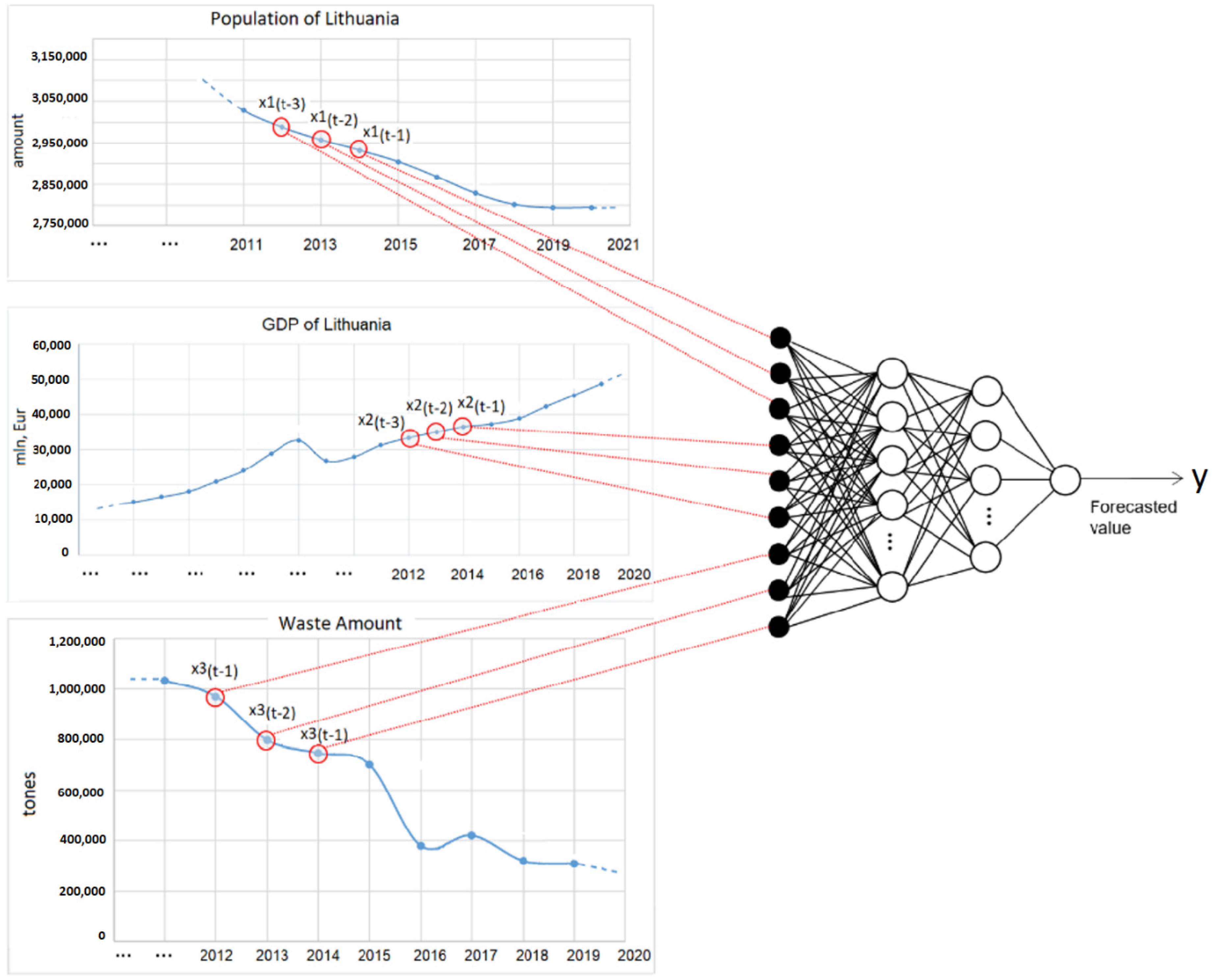
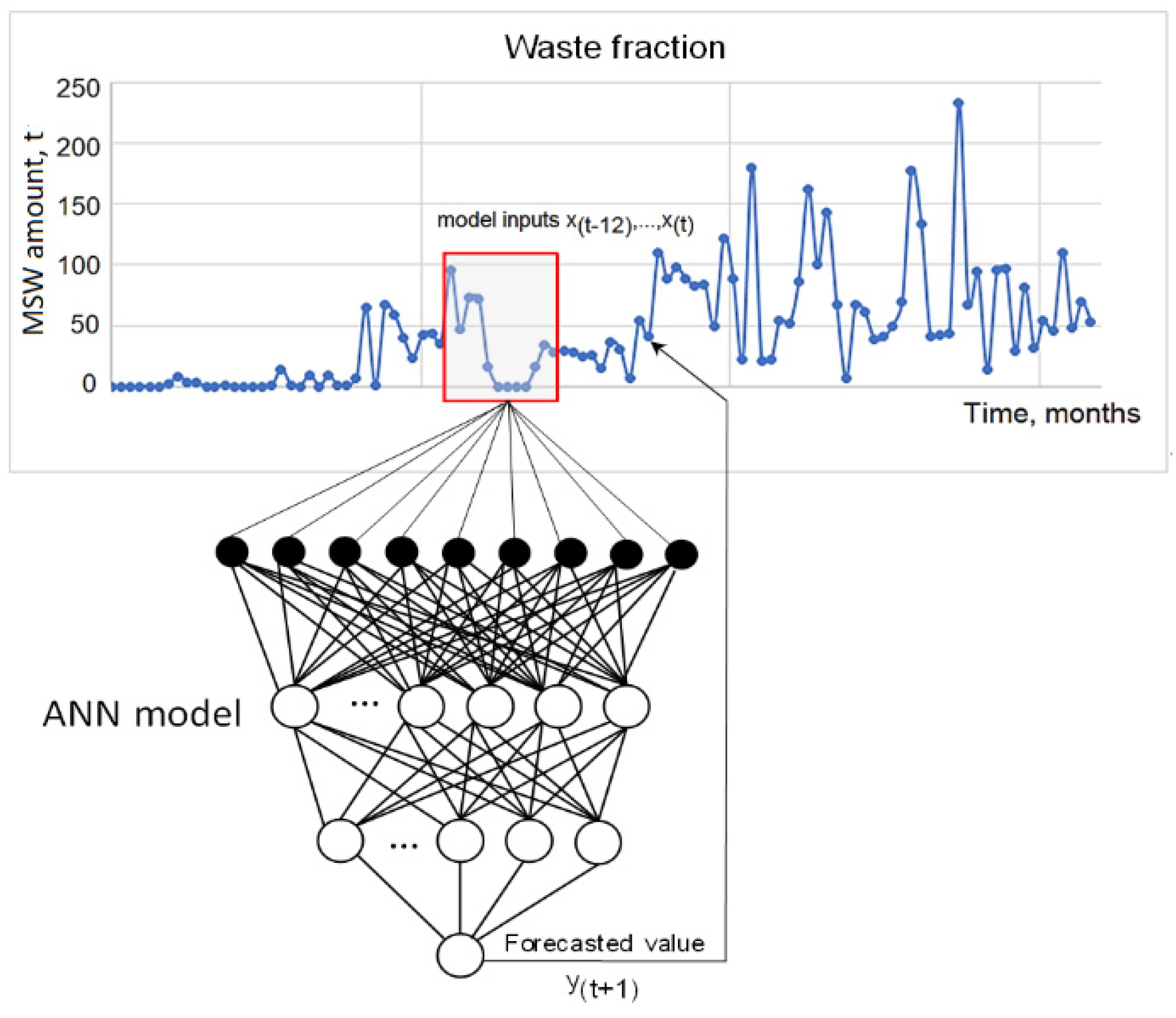
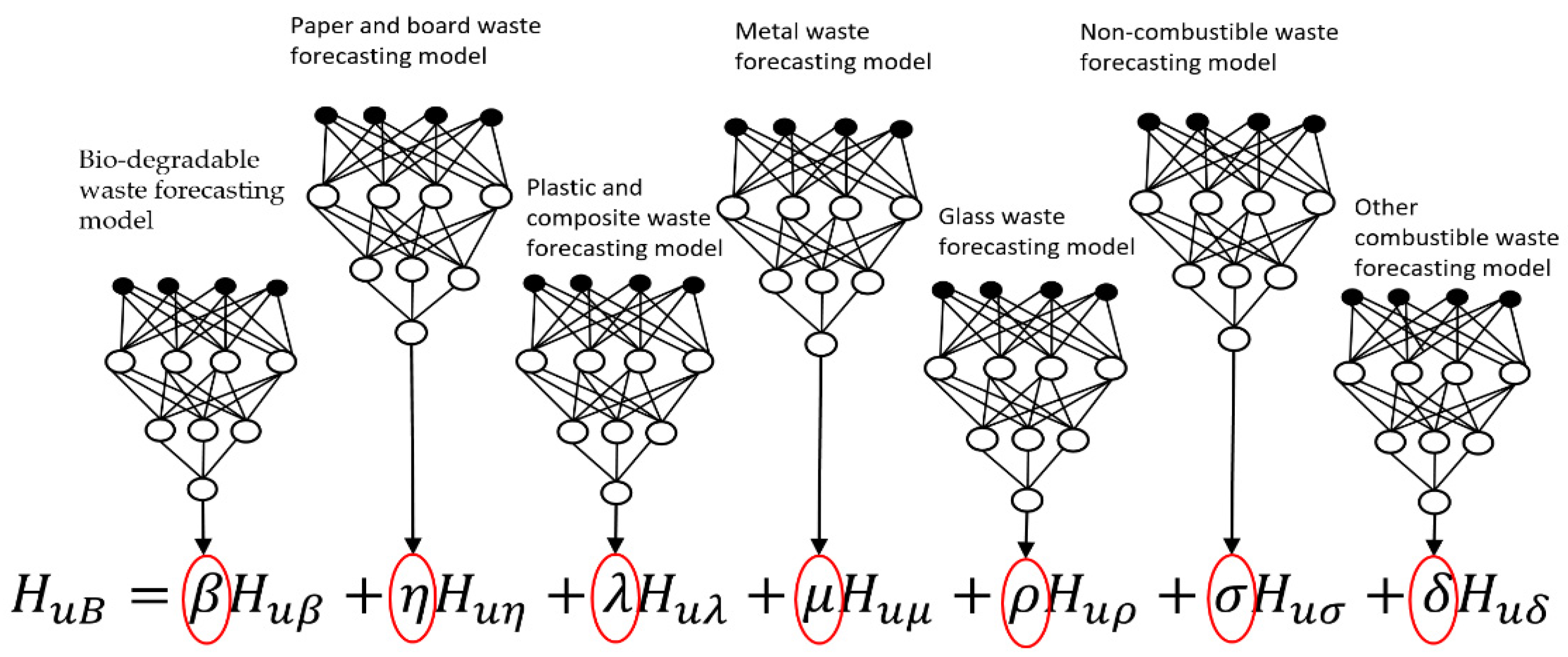
2.1. Model for Forecasting the Amount and Composition of MSW
2.2. Municipal Solid Waste to Energy
3. Results
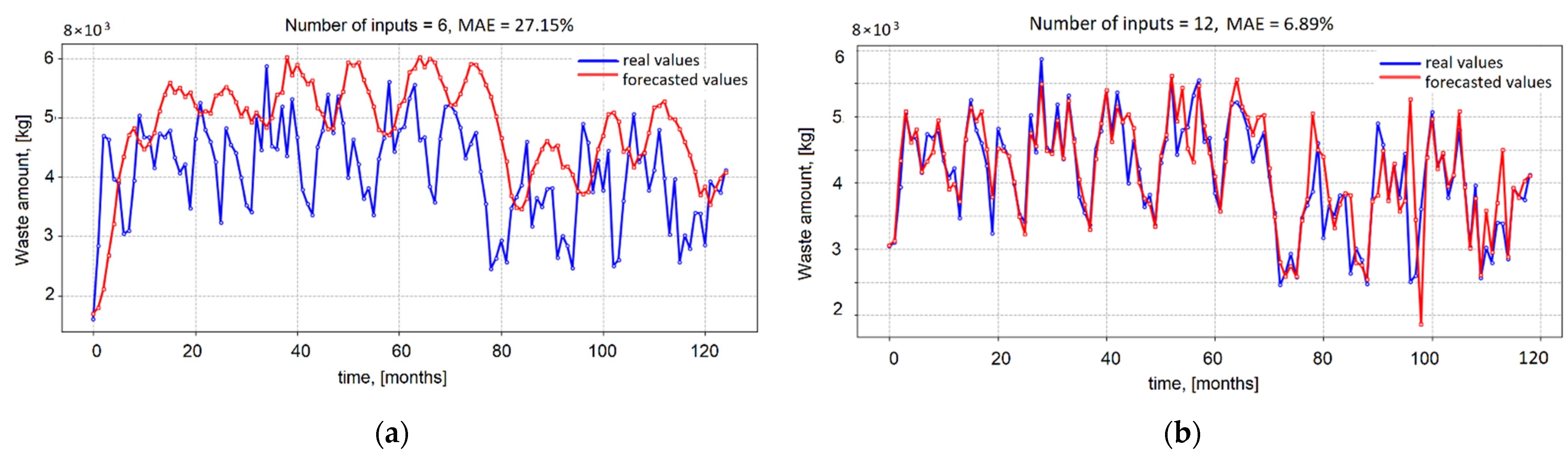
3.1. Estimation of Raw Material Recovery Potential Based-on the MSW Trends
3.2. Accuracy of Energy Forecasting
4. Discussion
5. Conclusions
Author Contributions
Funding
Institutional Review Board Statement
Informed Consent Statement
Data Availability Statement
Conflicts of Interest
References
- Chamas, A.; Moon, H.; Zheng, J.; Qiu, Y.; Tabassum, T.; Jang, J.H.; Abu-Omar, M.; Scott, S.L.; Suh, S. Degradation Rates of Plastics in the Environment. ACS Sustain. Chem. Eng. 2020, 8, 3494–3511. [Google Scholar] [CrossRef] [Green Version]
- Iqbal, A.; Liu, X.; Chena, G.H. Municipal solid waste: Review of best practices in application of life cycle assessment and sus-tainable management techniques. Sci. Total Environ. 2020, 729, 138622. [Google Scholar] [CrossRef] [PubMed]
- Popli, K.; Park, C.; Han, S.-M.; Kim, S. Prediction of Solid Waste Generation Rates in Urban Region of Laos Using Socio-Demographic and Economic Parameters with a Multi Linear Regression Approach. Sustainability 2021, 13, 3038. [Google Scholar] [CrossRef]
- Paulauskaite-Taraseviciene, A.; Raudonis, V.; Sutiene, K. Forecasting municipal solid waste in Lithuania by incorporating socioeconomic and geographical factors. Waste Manag. 2022, 140, 31–39. [Google Scholar] [CrossRef]
- Vieira, V.H.A.D.M.; Matheus, D.R. The impact of socioeconomic factors on municipal solid waste generation in São Paulo, Brazil. Waste Manag. Res. J. Sustain. Circ. Econ. 2017, 36, 79–85. [Google Scholar] [CrossRef] [PubMed] [Green Version]
- Mintz, K.K.; Henn, L.; Park, J.; Kurman, J. What predicts household waste management behaviors? Culture and type of behavior as moderators. Resour. Conserv. Recycl. 2019, 145, 11–18. [Google Scholar] [CrossRef]
- Pan, A.; Yu, L.; Yang, Q. Characteristics and Forecasting of Municipal Solid Waste Generation in China. Sustainability 2019, 11, 1433. [Google Scholar] [CrossRef] [Green Version]
- Vu, H.L.; Ng, K.T.W.; Bolingbroke, D. Time-lagged effects of weekly climatic and socio-economic factors on ANN municipal yard waste prediction models. Waste Manag. 2018, 84, 129–140. [Google Scholar] [CrossRef]
- Rosecký, M.; Šomplák, R.; Slavík, J.; Kalina, J.; Bulková, G.; Bednář, J. Predictive modelling as a tool for effective municipal waste management policy at different territorial levels. J. Environ. Manag. 2021, 291, 112584. [Google Scholar] [CrossRef]
- Wu, F.; Niu, D.; Dai, S.; Wu, B. New insights into regional differences of the predictions of municipal solid waste generation rates using artificial neural networks. Waste Manag. 2020, 107, 182–190. [Google Scholar] [CrossRef]
- Challcharoenwattana, A.; Pharino, C. Analysis of Socioeconomic and Behavioral Factors Influencing Participation in Community-Based Recycling Program: A Case of Peri-Urban Town in Thailand. Sustainability 2018, 10, 4500. [Google Scholar] [CrossRef] [Green Version]
- Abdallah, M.; Talib, A.; Feroz, S.; Nasir, Q.; Abdalla, H.; Mahfood, B. Artificial intelligence applications in solid waste man-agement: A systematic research review. Waste Manag. 2020, 109, 231–246. [Google Scholar] [CrossRef] [PubMed]
- Cucchiella, F.; D’Adamo, I.; Gastaldi, M. Sustainable waste management: Waste to energy plant as an alternative to landfill. Energy Convers. Manag. 2017, 131, 18–31. [Google Scholar] [CrossRef]
- Istrate, I.-R.; Iribarren, D.; Gálvez-Martos, J.-L.; Dufour, J. Review of life-cycle environmental consequences of waste-to-energy solutions on the municipal solid waste management system. Resour. Conserv. Recycl. 2020, 157, 104778. [Google Scholar] [CrossRef]
- Vlachokostas, C.; Michailidou, A.; Achillas, C. Multi-Criteria Decision Analysis towards promoting Waste-to-Energy Management Strategies: A critical review. Renew. Sustain. Energy Rev. 2020, 138, 110563. [Google Scholar] [CrossRef]
- Kannangara, M.; Dua, R.; Ahmadi, L.; Bensebaa, F. Modeling and prediction of regional municipal solid waste generation and diversion in Canada using machine learning approaches. Waste Manag. 2018, 74, 3–15. [Google Scholar] [CrossRef]
- Ceylan, Z. Estimation of municipal waste generation of Turkey using socio-economic indicators by Bayesian optimization tuned Gaussian process regression. Waste Manag. Res. J. Sustain. Circ. Econ. 2020, 38, 840–850. [Google Scholar] [CrossRef]
- Ponce, E.O.; Samarasinghe, S.; Torgerson, A. Model for assessing waste generation factors and forecasting waste generation using artificial neural networks: A case study of Chile. In Conference Proceedings of the Waste and Recycle, Fremantle, Australia, 21–24 September 2004; pp. 1–11. [Google Scholar]
- Ahuja, N.J.; Bahukhandi, K.D. Expert systems for Solid Waste Management: A Review. Int. Rev. Comput. Softw. 2012, 7, 1608–1613. [Google Scholar]
- Kokkinos, K.; Karayannis, V.; Lakioti, E.; Moustakas, K. Exploring social determinants of municipal solid waste management: Survey processing with fuzzy logic and self-organized maps. Environ. Sci. Pollut. Res. 2019, 26, 35288–35304. [Google Scholar] [CrossRef]
- Alberdi, E.; Urrutia, L.; Goti, A.; Oyarbide-Zubillaga, A. Modeling the Municipal Waste Collection Using Genetic Algorithms. Processes 2020, 8, 513. [Google Scholar] [CrossRef]
- Camero, A.; Toutouh, J.; Ferrer, J.; Alba, E. Waste generation prediction under uncertainty in smart cities through deep neuroevolution. Rev. Fac. Ing. Univ. Antioq. 2019, 93, 128–138. [Google Scholar] [CrossRef]
- Xu, A.; Chang, H.; Xu, Y.; Li, R.; Li, X.; Zhao, Y. Applying artificial neural networks (ANNs) to solve solid waste-related issues: A critical review. Waste Manag. 2021, 124, 385–402. [Google Scholar] [CrossRef] [PubMed]
- Araiza-Aguilar, J.; Rojas-Valencia, M.; Aguilar-Vera, R. Forecast generation model of municipal solid waste using multiple linear regression. Glob. J. Environ. Sci. Manag. 2020, 6, 1–14. [Google Scholar] [CrossRef]
- Cubillos, M.; Wulff, J.N.; Wøhlk, S. A multilevel Bayesian framework for predicting municipal waste generation rates. Waste Manag. 2021, 127, 90–100. [Google Scholar] [CrossRef]
- Kolekar, K.; Hazra, T.; Chakrabarty, S. A Review on Prediction of Municipal Solid Waste Generation Models. Procedia Environ. Sci. 2016, 35, 238–244. [Google Scholar] [CrossRef]
- Azarmi, S.L.; Oladipo, A.A.; Roozbeh, V.; Alipour, H. Comparative Modelling and Artificial Neural Network Inspired Pre-diction of Waste Generation Rates of Hospitality Industry: The Case of North Cyprus. Sustainability 2018, 10, 2965. [Google Scholar] [CrossRef] [Green Version]
- Vu, H.L.; Ng, K.T.W.; Richter, A.; Kabir, G. The use of a recurrent neural network model with separated time-series and lagged daily inputs for waste disposal rates modeling during COVID-19. Sustain. Cities Soc. 2021, 75, 103339. [Google Scholar] [CrossRef]
- Abbsi, M.; Hanandeh, A.E. Forecasting municipal solid waste generation using artificial intelligence modelling approaches. Waste Manag. 2016, 56, 13–22. [Google Scholar] [CrossRef]
- Lin, K.; Zhao, Y.; Kuo, J.H.; Deng, H.; Cui, F.; Zhang, Z.; Zhang, M.; Zhao, C.; Gao, X.; Zhou, T.; et al. Toward smarter management and recovery of municipal solid waste: A critical review on deep learning approaches. J. Clean. Prod. 2022, 346, 130943. [Google Scholar] [CrossRef]
- Huang, L.; Cai, T.; Zhu, Y.; Zhu, Y.; Wang, W.; Sun, K. LSTM-Based Forecasting for Urban Construction Waste Generation. Sustainability 2020, 12, 8555. [Google Scholar] [CrossRef]
- Zhang, Q.; Yang, Q.; Zhang, X.; Bao, Q.; Su, J.; Liu, X. Waste image classification based on transfer learning and convolutional neural network. Waste Manag. 2021, 135, 150–157. [Google Scholar] [CrossRef] [PubMed]
- Singh, M. Forecasting of waste-to-energy system: A case study of Faridabad, India. Energy Sources Part A Recover. Util. Environ. Eff. 2019, 42, 319–328. [Google Scholar] [CrossRef]
- Bagheri, M.; Esfilar, R.; Golchi, M.S.; Kennedy, C.A. A comparative data mining approach for the prediction of energy recovery potential from various municipal solid waste. Renew. Sustain. Energy Rev. 2019, 116, 109423. [Google Scholar] [CrossRef]
- Muawad, S.A.; Wedaa, S.A.; Abuelnuor, A.A.; Elemam, A.E.; Ali, A.M.; Aldin, A.S.; Osman, I.I. Waste- to- Energy Production of Alternative Energy Source Using Landfill Technology. In Proceedings of the International Conference on Computer, Control, Electrical, and Electronics Engineering (ICCCEEE), Khartoum, Sudan, 21–23 September 2019. [Google Scholar]
- Maynard, M. Neural Networks: Introduction to Artificial Neurons, Backpropagation and Multilayer Feedforward Neural Networks with Real-World Applications; Independently published; 2020; p. 42. ISBN 9798642783528. [Google Scholar]
- Botchkarev, A. Performance Metrics (Error Measures) in Machine Learning Regression, Forecasting and Prognostics: Properties and Typology, Interdisciplinary Journal of Information, Knowledge, and Management. arXiv 2019, arXiv:1809.03006. [Google Scholar]
- Menikpura, S.N.M.; Basnayake, B.F.A. New applications of ‘Hess Law’ and comparisons with models for determining calorific values of municipal solid wastes in the Sri Lankan context. Renew. Energy 2009, 34, 1587–1594. [Google Scholar] [CrossRef]
- Environmental Protection Encouragement Agency. Neue Ersatzbrennstoff-Anlagen—Kein Ersatz für Intelligentes Stoffstrommanagement; Independently Published: Norderstedt, Germany, 2007. [Google Scholar]
- Boer, E.; Boer, J.; Jager, J. Deliverable Report: Environmental Sustainability Criteria and Indicators for Waste Management The Use of Life Cycle Assessment Tool for the Development of Integrated Waste Management Strategies for Cities and Regions with Rapid Growing Economies; European Commission: Darmstadt, Germany, 2005. [Google Scholar]
- Cerbe, G.; Hoffmann, H.-J. Einführung in die Thermodynamik, 10th ed.; Carl Hanser Verlag: Munich/Vienna, Germany, 1994. [Google Scholar]
- Valaviciene, I. The Impact of Seasonal Variation of Municipal Waste Generation on Waste Management System Indicator. Ph.D. Thesis, Technological Sciences, Environmental Engineering and Landscape Management, Kaunas University of Technology, Kaunas, Lithuania, 2013; p. 109. [Google Scholar]
- Leap, J.N. An Investigation of the Effects of Correlation, Autocorrelation, and Sample Size in Classifier Fusion; Theses and Dissertations. 4023, BiblioScholar; Air Force Institute of Technology, Air Force University: Dayton, OH, USA, 2012; p. 122. ISBN 10:1288326947. [Google Scholar]
- Kiaulytė, A.; Denafas, G. Feasibility Assessment for Resource Recovery at Alytus Regional Landfill; Environmental Engineering; Kaunas University of Technology, Faculty of Chemical Technology, Kaunas University of Technology: Kaunas, Lithuania, 2015; pp. 1–60. [Google Scholar]

| Social-Economic Factors in the Region | Waste Amount in the Landfill | |
|---|---|---|
| Siauliai Region Aukstrakiai Landfill | Alytus Region Takniskiu Landfill | |
| Total amount of waste in Lithuanian landfills, tonnes | ||
| GDP, thousands Eur | ||
| GDP per capita, thousands Eur | ||
| Emigration, thousands | ||
| Immigration thousands | ||
| Employment, % | ||
| Unemployment, % | ||
| Population in the region, thousands | ||
| Research and development (R&D) per capita, Eur | ||
| Waste Fraction | Calorific Value, MJ/kg |
|---|---|
| Paper | |
| Plastic | |
| Plastic packages | |
| Bio-wastes | |
| Glass | |
| Metal | |
| Wood | |
| Textile, rubber, synthetic leather | |
| Other wastes (including mineral waste) | |
| Composites | |
| Composite packages |
| Lapes Lanfill | ||||||||||
|---|---|---|---|---|---|---|---|---|---|---|
| Metrics | Number of Inputs | |||||||||
| 6 | 7 | 8 | 9 | 10 | 11 | 12 | 13 | 14 | 15 | |
| 27.15% | 23.10% | 18.33% | 8.62% | 21.49% | 16.99% | 6.89% | ||||
| 26.50% | 22.80% | 17.20% | 7.25% | 20.78% | 14.90% | 5.73% | 6.89% | 9.80% | 7.36% | |
| −0.62 | −0.52 | −0.28 | 0.51 | −0.41 | −0.02 | 0.66 | 0.63 | 0.15 | 0.49 | |
| −0.65 | −0.58 | −0.31 | 0.61 | −0.45 | −0.01 | 0.71 | 0.65 | 0.17 | 0.53 | |
| Aukstrakiailandfill | ||||||||||
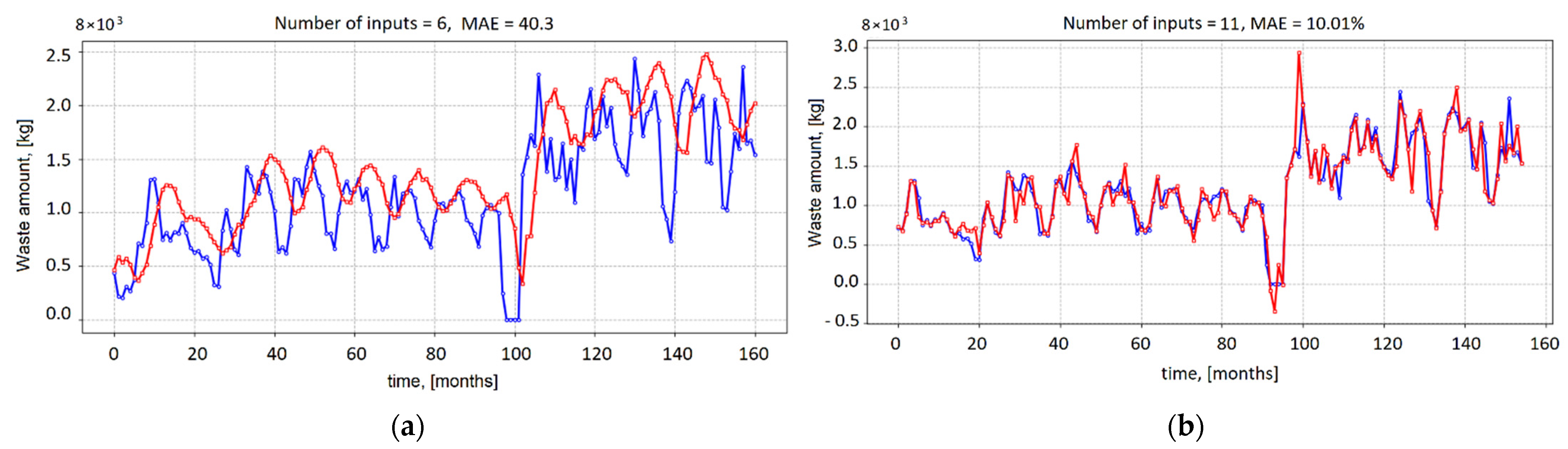
| 40.30% | 29.19% | 13.37% | 11.07% | 10.01% | 10.11% | 11.49% | 11.20% | 12.06% | ||
| 39.20% | 28.32% | 11.80% | 9.50% | 28.50% | 8.25% | 8.95% | 10.62% | 10.45% | 11.80% | |
| 0.17 | 0.51 | 0.78 | 0.86 | 0.37 | 0.85 | 0.91 | 0.82 | 0.84 | 0.81 | |
| 0.19 | 0.54 | 0.81 | 0.91 | 0.42 | 0.87 | 0.95 | 0.84 | 0.87 | 0.85 | |
| Year | Real Value, GWh/y | Forecasted Energy Values, GWh/y | |||||||
|---|---|---|---|---|---|---|---|---|---|
| 5 Inputs | 6 Inputs | 7 Inputs | 8 Inputs | 9 Inputs | 10 Inputs | 11 Inputs | 12 Inputs | ||
| 1 January 2007 | 0.25 | 0.92 | 0.66 | 0.71 | 0.60 | 0.53 | 0.77 | 0.70 | 0.66 |
| 1 January 2008 | 0.70 | 1.12 | 0.79 | 0.89 | 0.78 | 1.05 | 0.99 | 0.95 | 0.94 |
| 1 January 2009 | 1.47 | 3.36 | 2.28 | 2.78 | 2.35 | 2.90 | 2.99 | 2.33 | 2.29 |
| 1 January 2010 | 2.33 | 2.59 | 2.79 | 2.90 | 1.94 | 2.12 | 2.75 | 1.98 | 2.21 |
| 1 January 2011 | 2.09 | 2.81 | 2.40 | 2.71 | 2.33 | 2.52 | 2.60 | 2.45 | 2.33 |
| 1 January 2012 | 3.14 | 3.52 | 3.12 | 3.92 | 2.93 | 3.18 | 3.55 | 3.28 | 3.22 |
| 1 January 2013 | 6.84 | 7.02 | 6.53 | 6.92 | 5.95 | 5.35 | 6.37 | 6.12 | 6.52 |
| 1 January 2014 | 7.86 | 8.58 | 9.19 | 8.75 | 8.11 | 9.13 | 8.20 | 8.11 | 8.64 |
| 1 January 2015 | 4.86 | 5.11 | 5.98 | 6.54 | 6.20 | 6.78 | 6.62 | 6.36 | 5.96 |
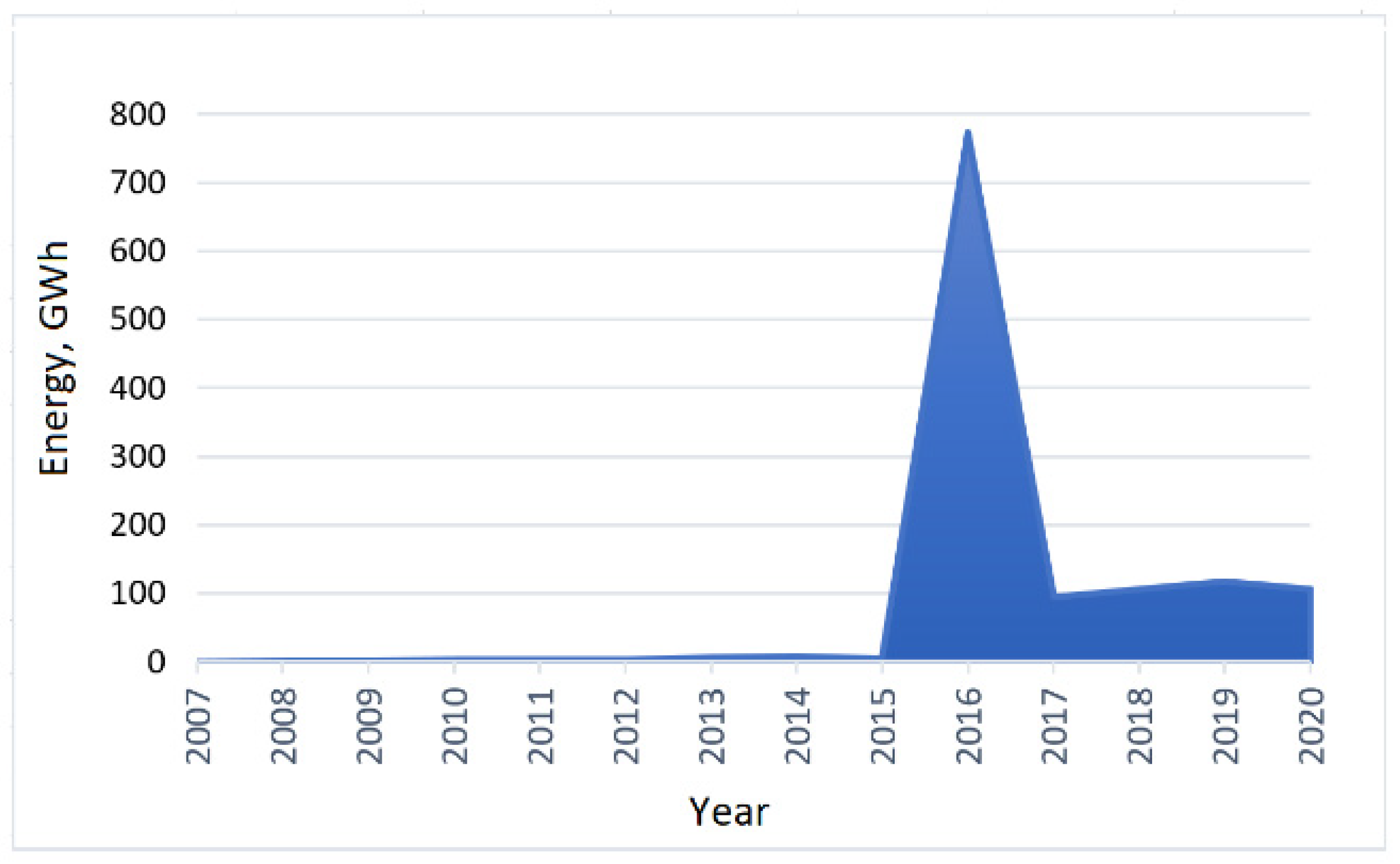
| 1 January 2016 | 773.20 | 602.52 | 762.76 | 635.31 | 754.06 | 642.26 | 644.89 | 712.58 | 709.93 |
| 1 January 2017 | 94.13 | 170.94 | 141.41 | 93.82 | 161.22 | 141.17 | 153.96 | 132.79 | 124.87 |
| 1 January 2018 | 105.80 | 121.03 | 90.16 | 100.46 | 118.21 | 96.41 | 93.03 | 109.93 | 112.15 |
| 1 January 2019 | 117.14 | 90.23 | 107.39 | 110.51 | 118.21 | 115.58 | 114.65 | 112.43 | 113.25 |
| 1 January 2020 | 105.81 | 89.40 | 82.67 | 73.48 | 92.68 | 90.83 | 81.79 | 90.69 | 88.34 |
| MAE | 22.25 | 7.936 | 13.506 | 8.391 | 15.095 | 16.69 | 9.151429 | 8.987857 | |
| MAPE | 49.1% | 29.2% | 31.8% | 27.8% | 32.8% | 40.9% | 30.5% | 17.1% | |
| Fraction | Actual Values, % | Forecasted Values, % | |||
|---|---|---|---|---|---|
| Waste Composition, % (Morphological Analysis) | ARIMA Model [31] | Regression Model | ANN + Waste Degradation | ANN 2021–2022 | |
| Paper | 0.96 | 11.03 | 2.71 | 2.254 | 1.866 |
| Glass | 0.25 | 7.23 | 2.05 | 0.485 | 0.351 |
| Metal | 3.6 | 2.44 | 0.85 | 1.537 | 1.932 |
| Plastic | 21.36 | 9.56 | 4.26 | 5.637 | 4.025 |
| Dangerous waste | 0.06 | 3.35 | 0.1 | 0.022 | 0 |
| Other non-combustible waste | 2.46 | 30.26 | 5.41 | 4.49 | 3.772 |
| Other combustible wastes | 24.62 | 14.55 | 46.66 | 25.86 | 27.051 |
| Fine fraction | 46.23 | 13.56 | None | 43.088 | 42.176 |
| Wood | 0.46 | 0 | 1.48 | 0.43 | 0.496 |
| Textile | 24.62 | 0 | 4.7 | 16.736 | 18.931 |
| Average MAE | 12.892 | 7.708 | 3.368 | ||
Publisher’s Note: MDPI stays neutral with regard to jurisdictional claims in published maps and institutional affiliations. |
© 2022 by the authors. Licensee MDPI, Basel, Switzerland. This article is an open access article distributed under the terms and conditions of the Creative Commons Attribution (CC BY) license (https://creativecommons.org/licenses/by/4.0/).
Share and Cite
Raudonis, V.; Paulauskaite-Taraseviciene, A.; Eidimtas, L. ANN Hybrid Model for Forecasting Landfill Waste Potential in Lithuania. Sustainability 2022, 14, 4122. https://doi.org/10.3390/su14074122
Raudonis V, Paulauskaite-Taraseviciene A, Eidimtas L. ANN Hybrid Model for Forecasting Landfill Waste Potential in Lithuania. Sustainability. 2022; 14(7):4122. https://doi.org/10.3390/su14074122
Chicago/Turabian StyleRaudonis, Vidas, Agne Paulauskaite-Taraseviciene, and Linas Eidimtas. 2022. "ANN Hybrid Model for Forecasting Landfill Waste Potential in Lithuania" Sustainability 14, no. 7: 4122. https://doi.org/10.3390/su14074122
APA StyleRaudonis, V., Paulauskaite-Taraseviciene, A., & Eidimtas, L. (2022). ANN Hybrid Model for Forecasting Landfill Waste Potential in Lithuania. Sustainability, 14(7), 4122. https://doi.org/10.3390/su14074122