
Hybrid Data-Driven Models for Hydrological Simulation and Projection on the Catchment Scale

 , ,
, ,  ,
, 
 ,
,  ,
,  ,
, 
Abstract
:1. Introduction
2. Materials and Methods
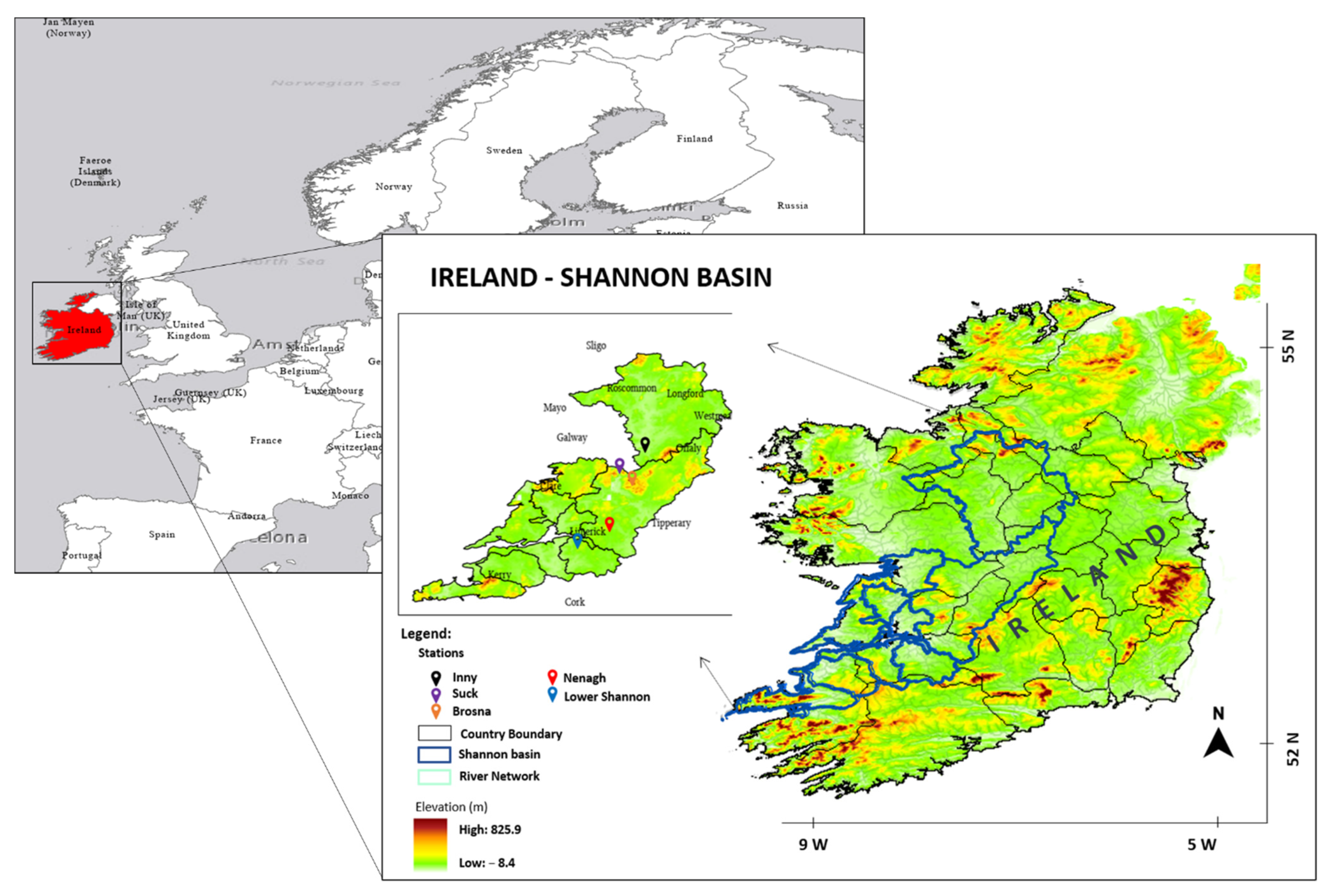
2.1. Catchment Description
2.2. Data Setup and Hydrometric Stations
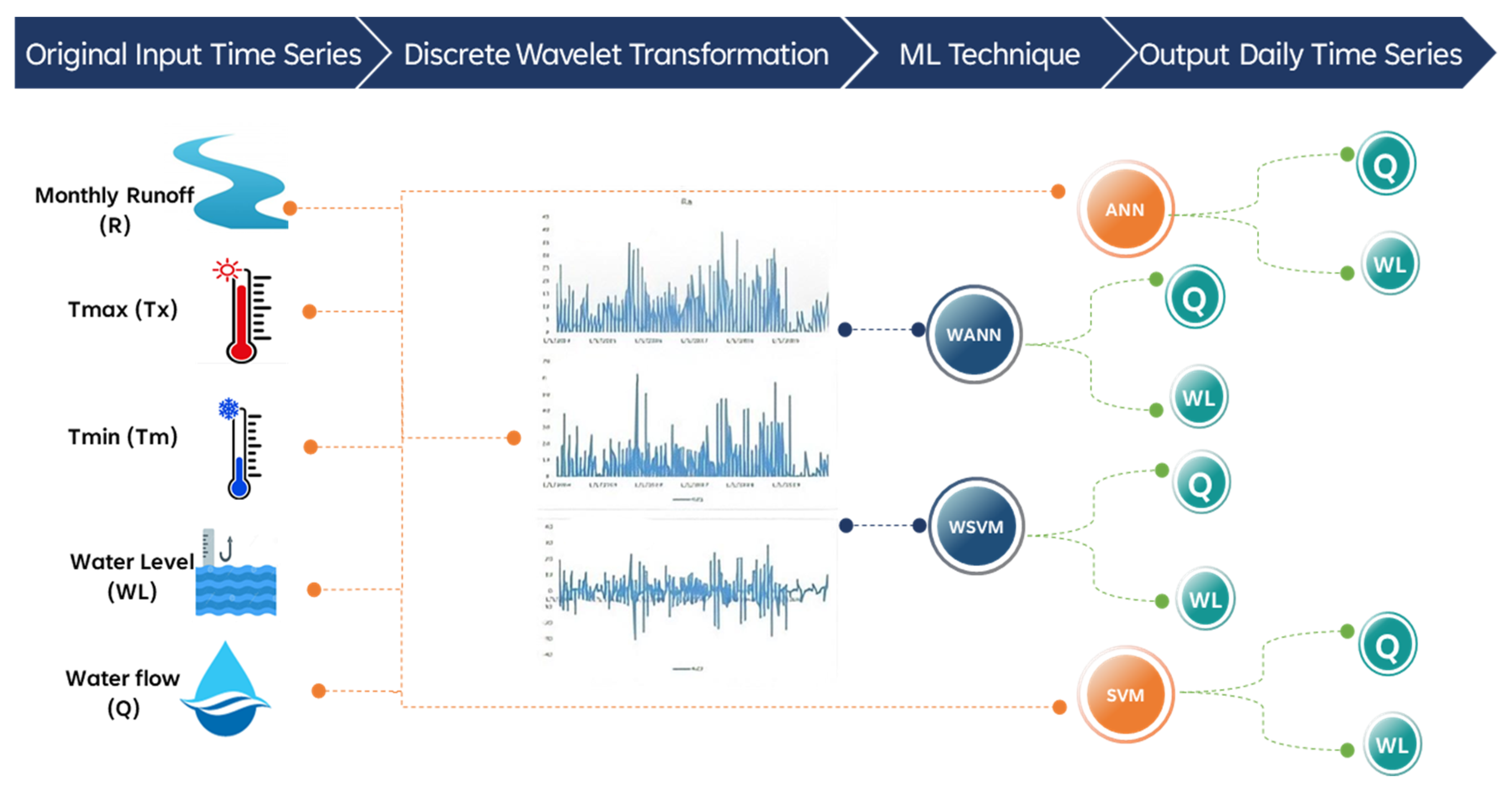
2.3. Workflow and Framework
2.4. Artificial Neural Network (ANN)
2.5. Support Vector Machine Regression (SVR)
2.6. Wavelet Transformation
2.6.1. Wavelet-ANN
2.6.2. Wavelet-SVR
2.7. Validation and Performance Evaluation
2.8. Lag Value
3. Results and Discussion
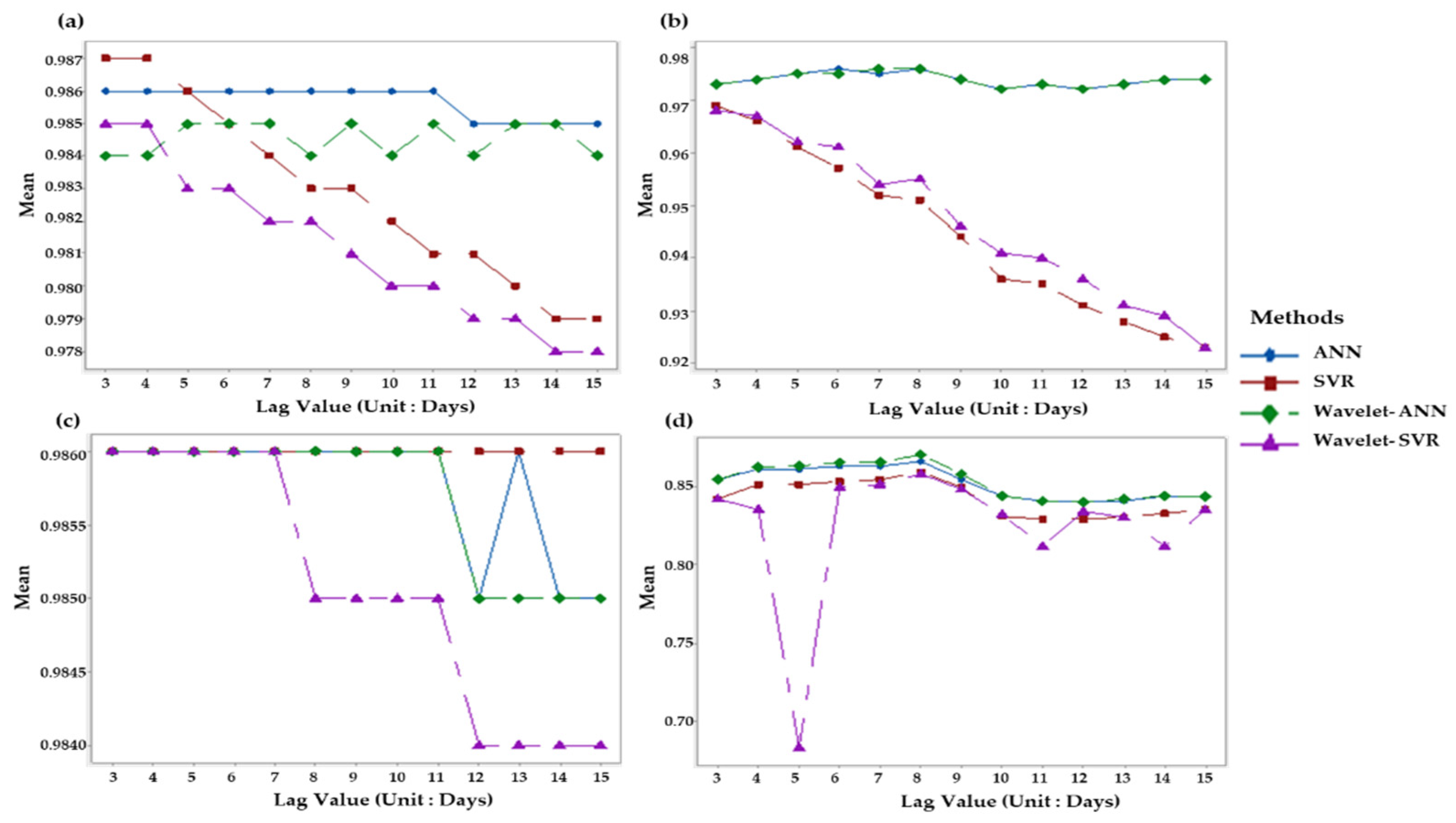
3.1. Simulated Models Using Different Lag Values
3.1.1. Water Flow Models Lag Value
3.1.2. Water Level Models Lag Value
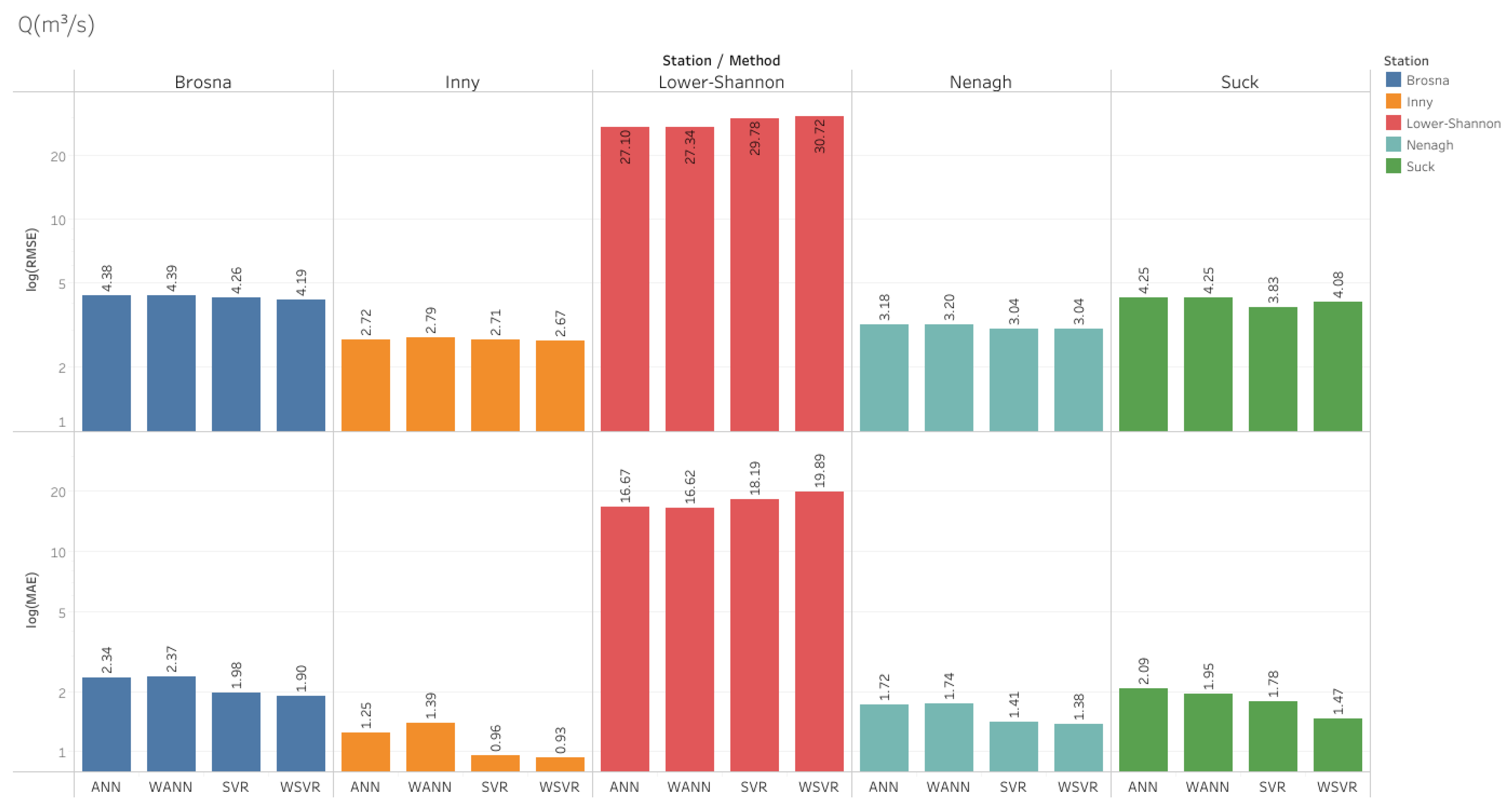
3.2. Model Evaluation
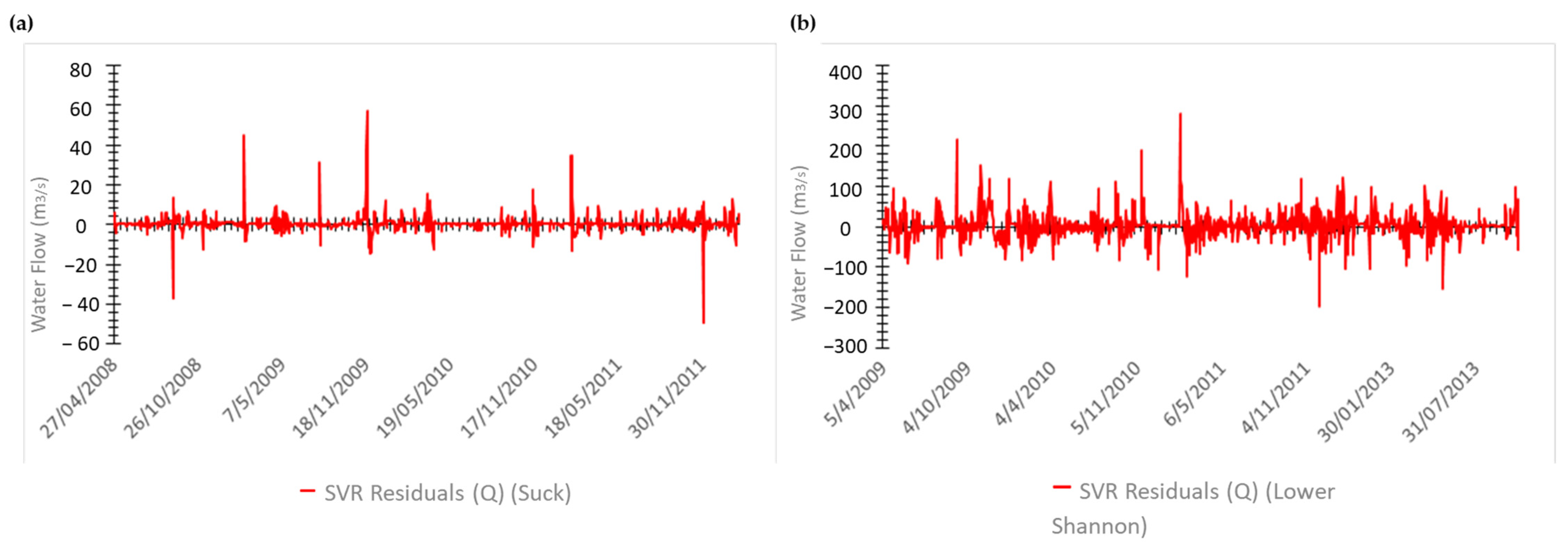
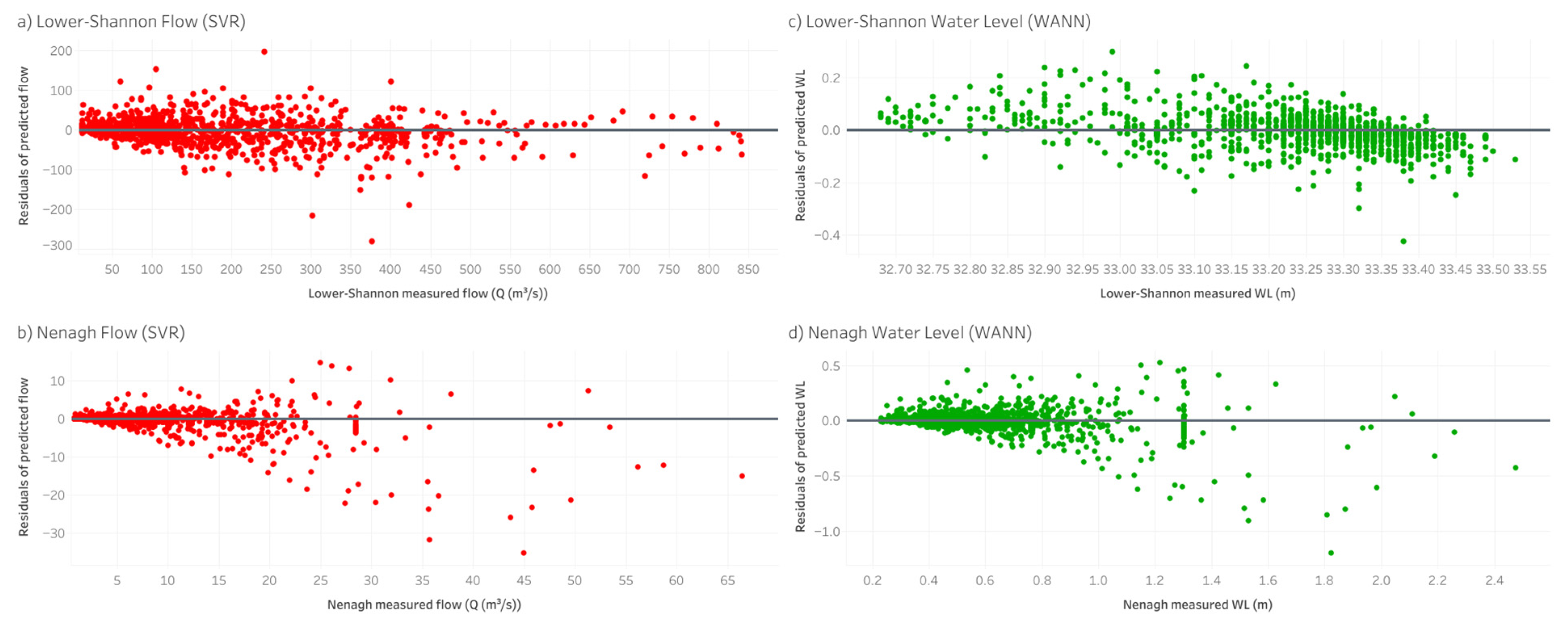
3.2.1. Flow Evaluation
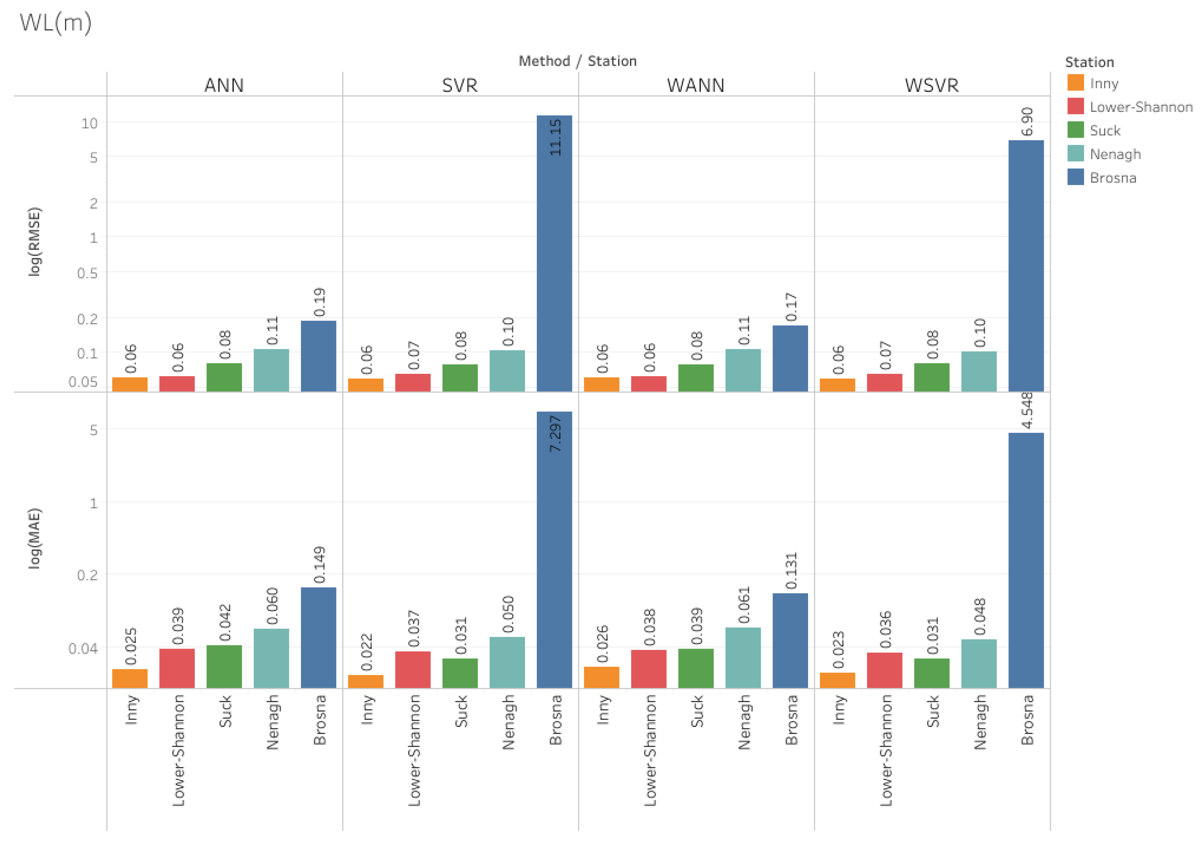
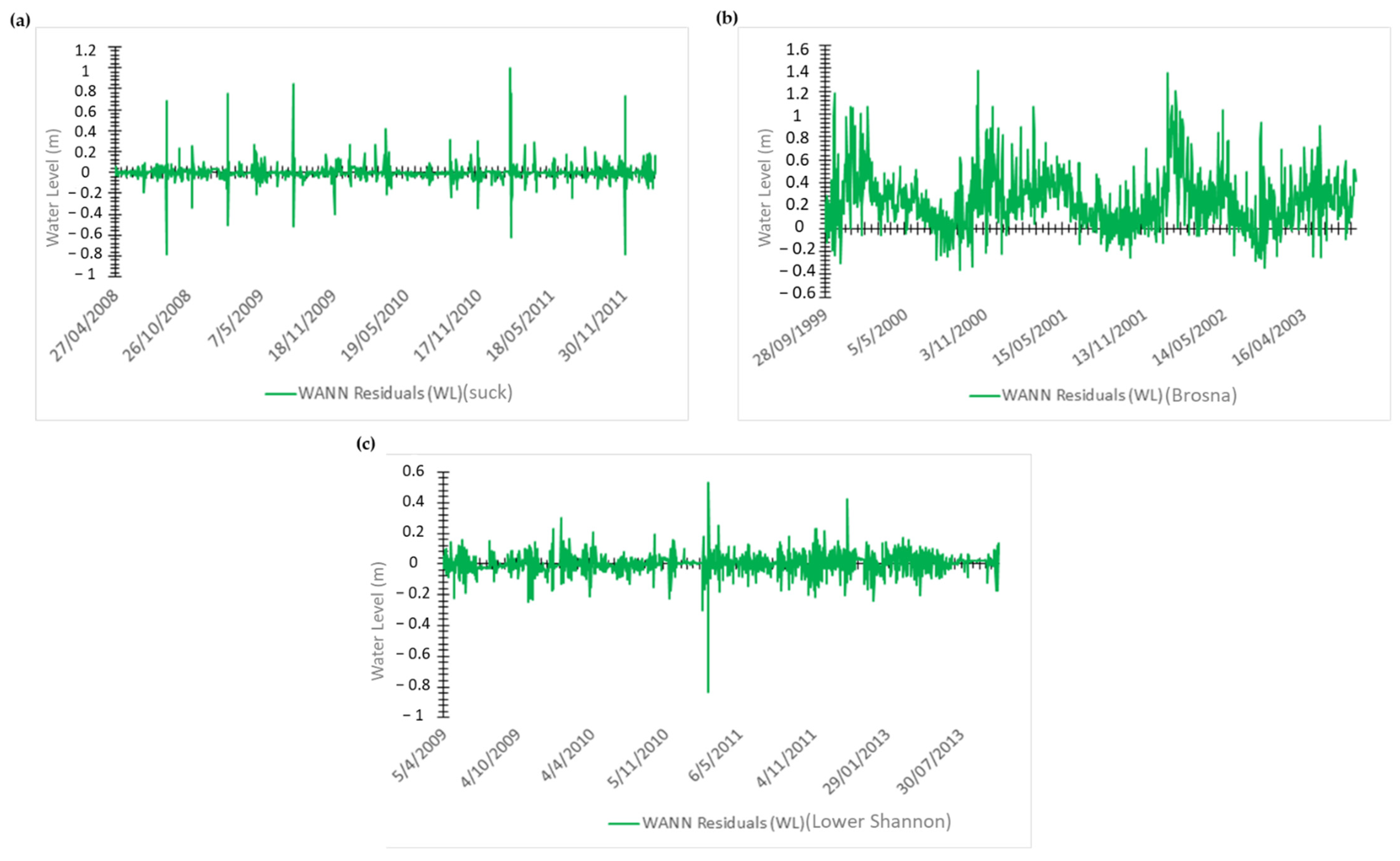
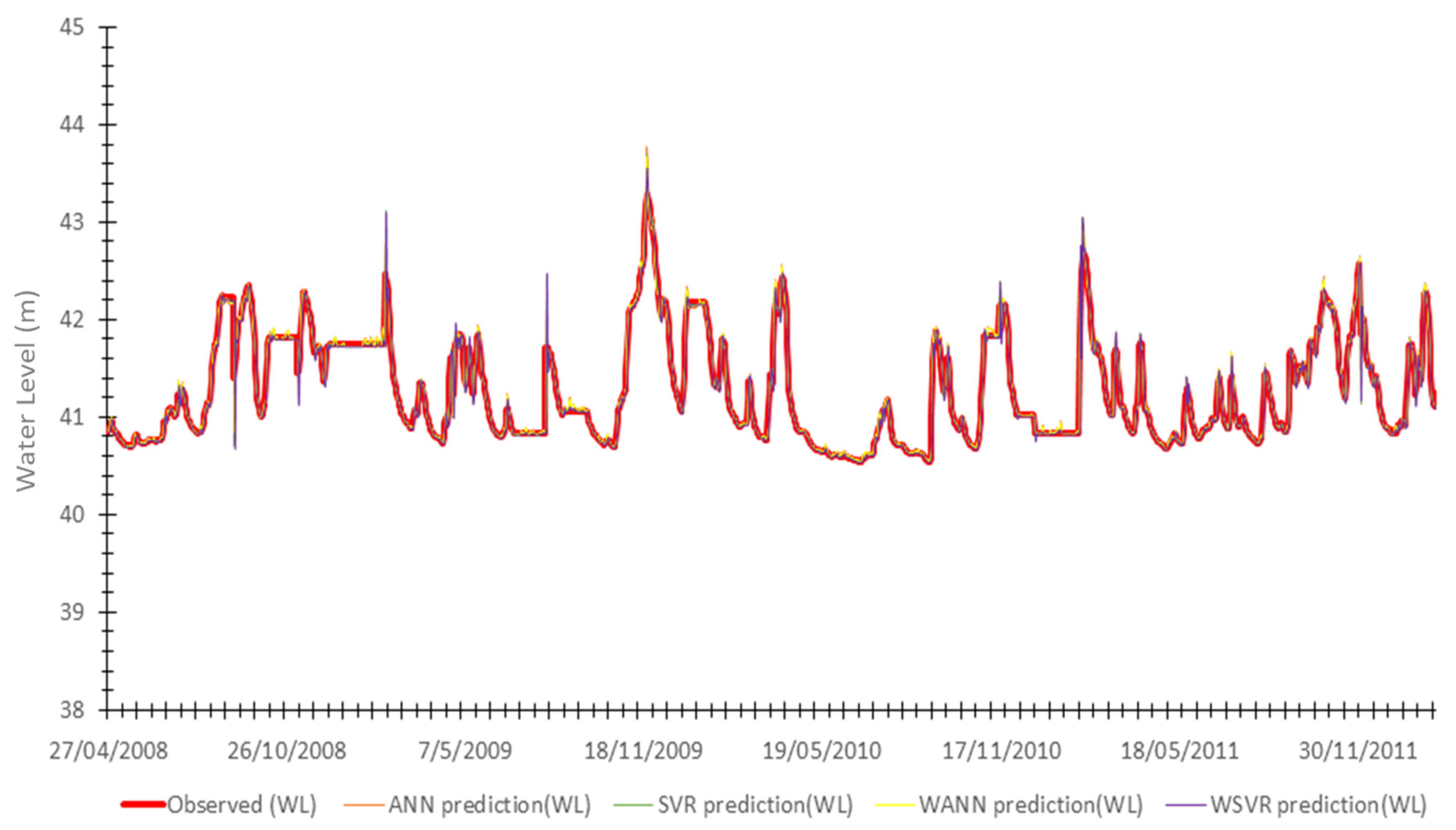
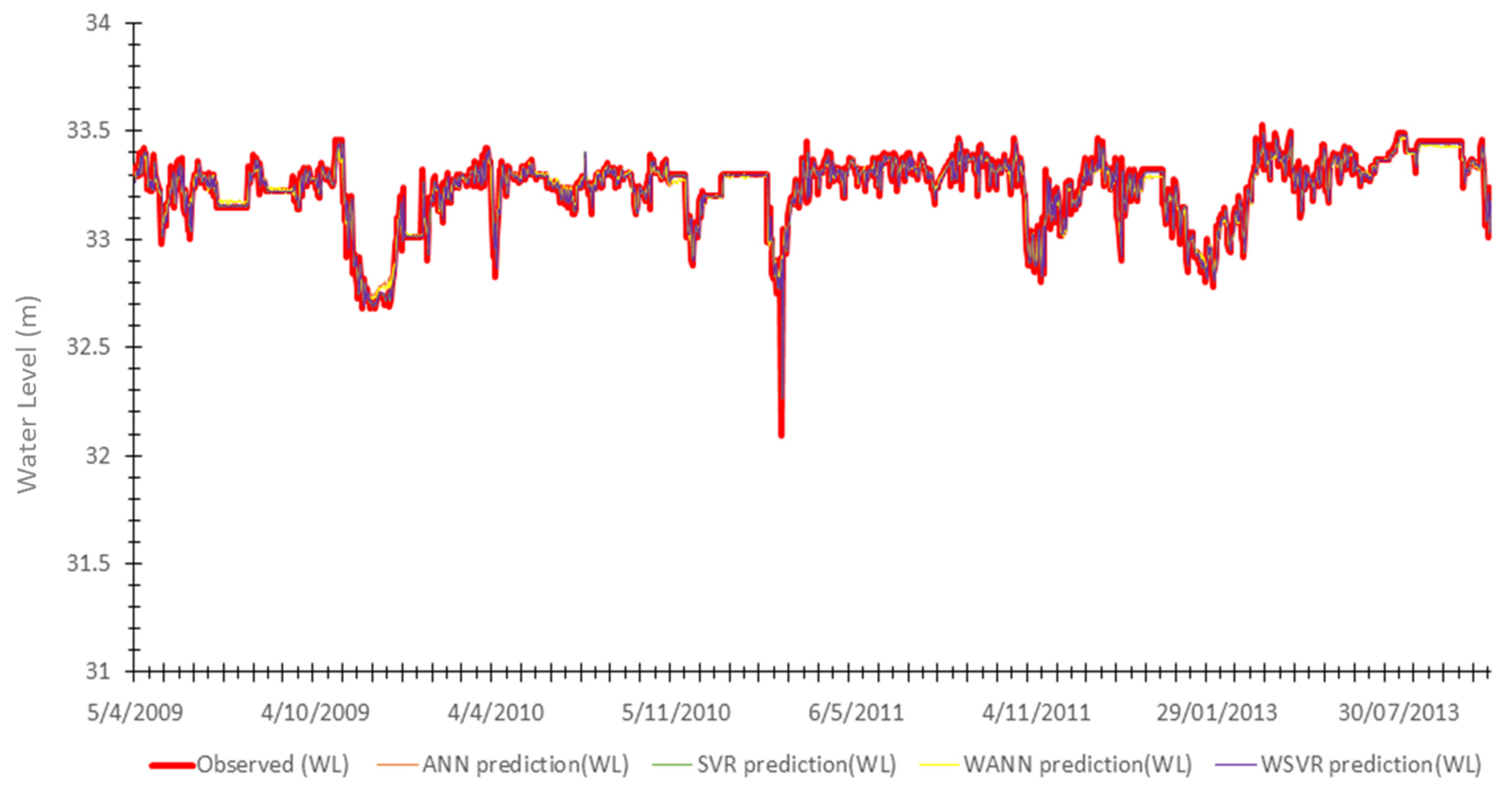
3.2.2. Water Level Evaluation
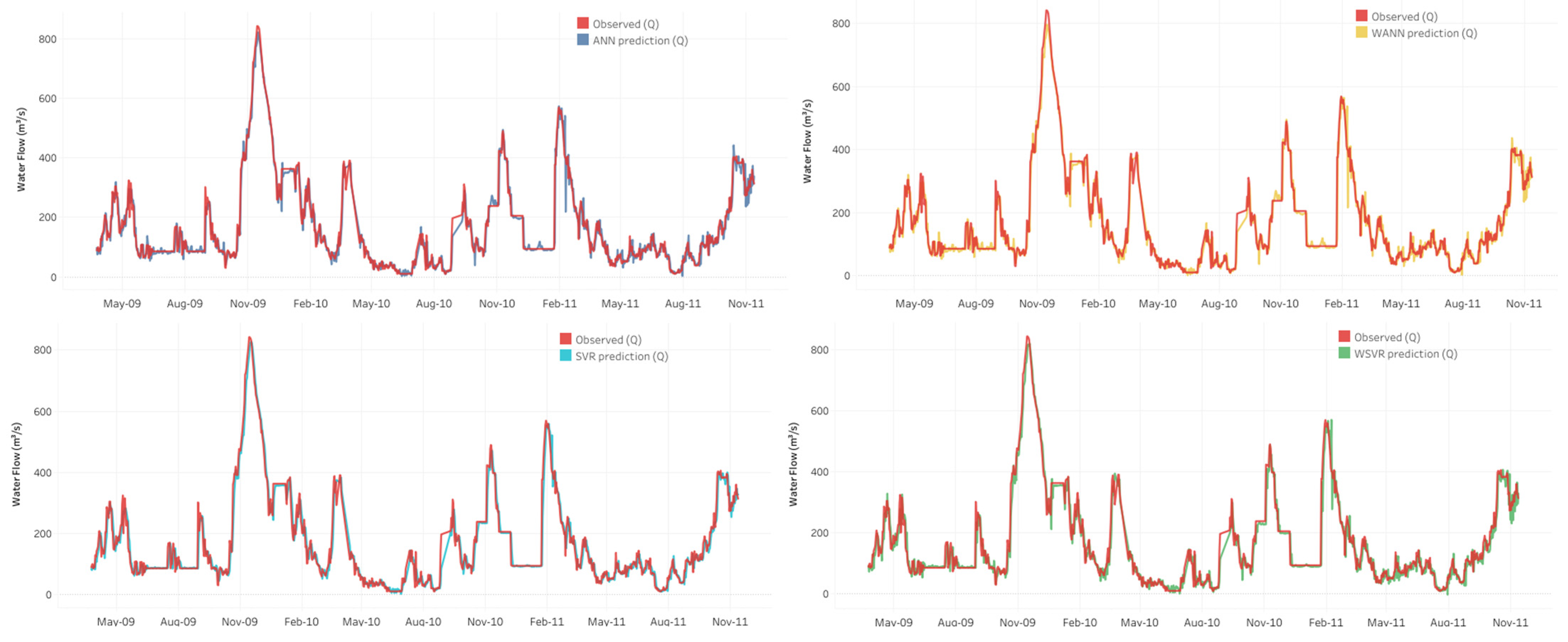
3.3. Flow Simulation
3.4. Water Level Simulation
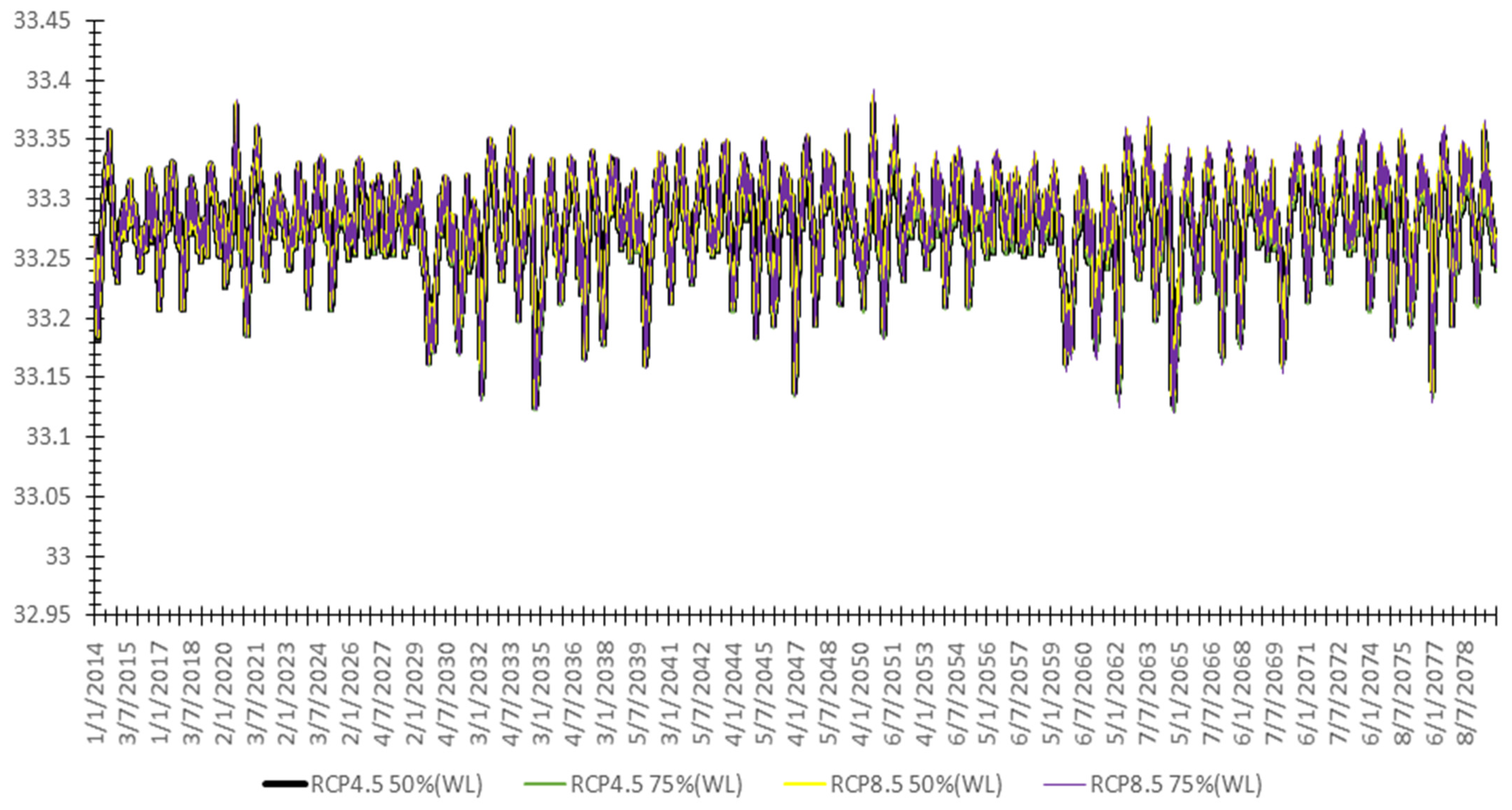
3.5. Projections Based on Climate Change Scenarios
4. Conclusions
Author Contributions
Funding
Institutional Review Board Statement
Informed Consent Statement
Data Availability Statement
Acknowledgments
Conflicts of Interest
Abbreviations
| ANN | Artificial Neural Networks |
| ARIMA | Autoregressive Integrated Moving Average |
| C | Cost |
| CWT | Continuous Wavelet Transform |
| DWT | Discrete Wavelet Transform |
| GEO-CWB | Geographical Spatially Distributed Water Balance Model |
| GHG | Greenhouse Gas |
| IPCC | Intergovernmental Panel on Climate Change |
| IQR | The Interquartile Range |
| MAE | Mean Absolute Error |
| MLR | Multiple Linear Regression |
| MSSD | Mean of the Squared Successive Difference |
| Q | Water Flow |
| Q1 | The First Quarter |
| Q3 | The Third Quarter |
| R | The Correlation Coefficient |
| R2 | The Coefficient of Determination |
| RBF | The Radial Basis Function |
| RCP | Representative Concentration Pathways |
| RMSE | Root Mean Square Error |
| SRE | Special Report on Emissions Scenarios |
| SSQ | The Uncorrected Sum of Squares |
| SVM | Support Vector Machine |
| SVR | Support Vector Machine Regression |
| TRMean | The Mean of the Data |
| Tmax | Maximum Temperature |
| Tmin | Minimum Temperature |
| WANN | Wavelet Artificial Neural Network |
| WL | Water Level |
| WSVR | Wavelet Support Vector Machine Regression |
Appendix A

| Station | Parameters | Datasets | Mean | SEMean | StDev | Variance | Q1 | Median | Q3 | IQR | TRMean | Min. | Max. | Range | Skewness | Kurtosis | MSSD | N |
|---|---|---|---|---|---|---|---|---|---|---|---|---|---|---|---|---|---|---|
| Inny | Daily average Tmax (°C) | Training | 13.895 | 0.058 | 5.108 | 26.090 | 10.200 | 13.500 | 17.600 | 7.400 | 13.843 | −1.500 | 30.600 | 32.100 | 0.159 | −0.391 | 2.488 | 7697 |
| Testing | 14.212 | 0.120 | 5.246 | 27.523 | 10.700 | 14.500 | 18.500 | 7.800 | 14.366 | −6.500 | 28.000 | 34.500 | −0.420 | −0.041 | 2.432 | 1925 | ||
| Daily average T min (°C) | Training | 5.525 | 0.058 | 5.082 | 25.829 | 1.700 | 5.700 | 9.500 | 7.800 | 5.579 | −8.900 | 18.300 | 27.200 | −0.145 | −0.666 | 6.974 | 7697 | |
| Testing | 5.313 | 0.126 | 5.513 | 30.389 | 1.000 | 6.000 | 9.900 | 8.900 | 5.447 | −14.000 | 17.100 | 31.100 | −0.324 | −0.572 | 7.594 | 1925 | ||
| Daily average simulated runoff (mm) | Training | 2.547 | 0.051 | 4.490 | 20.163 | 0.000 | 0.600 | 3.200 | 3.200 | 1.874 | 0.000 | 65.000 | 65.000 | 3.538 | 20.781 | 16.360 | 7697 | |
| Testing | 2.765 | 0.113 | 4.939 | 24.396 | 0.000 | 0.600 | 3.600 | 3.600 | 1.993 | 0.000 | 40.500 | 40.500 | 3.257 | 14.115 | 19.530 | 1925 | ||
| Daily average water level (mm) | Training | 45.471 | 0.004 | 0.372 | 0.138 | 45.140 | 45.398 | 45.716 | 0.576 | 45.450 | 44.923 | 47.124 | 2.201 | 0.786 | −0.015 | 0.002 | 7697 | |
| Testing | 45.531 | 0.010 | 0.453 | 0.205 | 45.140 | 45.357 | 45.802 | 0.662 | 45.503 | 44.996 | 47.294 | 2.298 | 0.925 | −0.286 | 0.002 | 1925 | ||
| Daily average water flow (m3/s) | Training | 16.988 | 0.165 | 14.479 | 209.644 | 5.070 | 12.341 | 24.476 | 19.406 | 15.661 | 1.656 | 104.231 | 102.575 | 1.355 | 1.951 | 3.542 | 7697 | |
| Testing | 18.453 | 0.391 | 17.154 | 294.249 | 5.070 | 10.911 | 25.745 | 20.675 | 17.044 | 2.543 | 105.846 | 103.303 | 1.302 | 0.839 | 3.400 | 1925 | ||
| Suck | Daily average T max (°C) | Training | 14.173 | 0.058 | 4.983 | 24.827 | 10.500 | 14.000 | 18.000 | 7.500 | 14.139 | −3.000 | 30.300 | 33.300 | 0.102 | −0.430 | 2.467 | 7303 |
| Testing | 13.922 | 0.129 | 5.520 | 30.467 | 10.200 | 14.000 | 18.200 | 8.000 | 14.014 | −6.500 | 29.200 | 35.700 | −0.236 | −0.192 | 2.573 | 1826 | ||
| Daily average T min (°C) | Training | 5.723 | 0.059 | 5.014 | 25.136 | 2.000 | 6.000 | 9.700 | 7.700 | 5.789 | −8.600 | 18.300 | 26.900 | −0.179 | −0.668 | 7.118 | 7303 | |
| Testing | 5.252 | 0.133 | 5.673 | 32.178 | 0.900 | 5.850 | 9.900 | 9.000 | 5.369 | −14.000 | 17.500 | 31.500 | −0.285 | −0.621 | 7.152 | 1826 | ||
| Daily average simulated runoff (mm) | Training | 2.752 | 0.055 | 4.698 | 22.069 | 0.000 | 0.600 | 3.700 | 3.700 | 2.053 | 0.000 | 61.800 | 61.800 | 3.057 | 14.385 | 17.800 | 7303 | |
| Testing | 3.053 | 0.126 | 5.397 | 29.130 | 0.000 | 0.500 | 4.000 | 4.000 | 2.230 | 0.000 | 49.400 | 49.400 | 3.172 | 14.133 | 22.321 | 1826 | ||
| Daily average water level (mm) | Training | 41.201 | 0.006 | 0.513 | 0.263 | 40.855 | 40.946 | 41.519 | 0.664 | 41.163 | 40.540 | 42.782 | 2.242 | 1.092 | 0.010 | 0.004 | 7303 | |
| Testing | 41.409 | 0.016 | 0.673 | 0.453 | 40.855 | 41.095 | 41.841 | 0.986 | 41.385 | 40.544 | 43.279 | 2.735 | 0.683 | −0.944 | 0.004 | 1826 | ||
| Daily flow volume (m3/s) | Training | 20.867 | 0.253 | 21.613 | 467.104 | 5.589 | 10.763 | 30.382 | 24.793 | 18.522 | 1.140 | 123.518 | 122.378 | 1.542 | 1.762 | 7.313 | 7303 | |
| Testing | 32.055 | 0.773 | 33.032 | 1091.110 | 6.101 | 15.960 | 42.920 | 36.819 | 29.744 | 1.493 | 221.214 | 219.721 | 1.360 | 1.788 | 8.952 | 1826 | ||
| Brosna | Daily average T max (°C) | Training | 13.746 | 0.074 | 5.179 | 26.824 | 10.000 | 13.500 | 17.500 | 7.500 | 13.714 | −3.000 | 30.600 | 33.600 | 0.089 | −0.367 | 2.590 | 4844 |
| Testing | 13.872 | 0.142 | 4.927 | 24.275 | 10.300 | 13.600 | 17.600 | 7.300 | 13.875 | −1.500 | 29.200 | 30.700 | 0.028 | −0.470 | 2.422 | 1211 | ||
| Daily average T min (°C) | Training | 5.482 | 0.074 | 5.130 | 26.322 | 1.600 | 5.600 | 9.500 | 7.900 | 5.543 | −9.000 | 18.000 | 27.000 | −0.156 | −0.672 | 7.101 | 4844 | |
| Testing | 5.459 | 0.145 | 5.030 | 25.304 | 1.600 | 5.600 | 9.400 | 7.800 | 5.519 | −7.800 | 17.000 | 24.800 | −0.148 | −0.644 | 6.503 | 1211 | ||
| Daily average simulated runoff (mm) | Training | 2.499 | 0.067 | 4.664 | 21.754 | 0.000 | 0.300 | 3.000 | 3.000 | 1.777 | 0.000 | 57.000 | 57.000 | 3.488 | 18.270 | 18.106 | 4844 | |
| Testing | 2.369 | 0.121 | 4.216 | 17.771 | 0.000 | 0.400 | 3.200 | 3.200 | 1.731 | 0.000 | 38.100 | 38.100 | 3.248 | 15.421 | 15.976 | 1211 | ||
| Daily average water level (mm) | Training | 40.375 | 0.136 | 9.472 | 89.712 | 42.155 | 42.433 | 42.806 | 0.651 | 42.423 | 0.000 | 45.056 | 45.056 | −4.018 | 14.204 | 9.010 | 4844 | |
| Testing | 42.574 | 0.015 | 0.527 | 0.278 | 42.186 | 42.398 | 42.748 | 0.562 | 42.522 | 41.941 | 44.662 | 2.721 | 1.423 | 1.690 | 0.009 | 1211 | ||
| Daily flow volume (m3/s) | Training | 17.972 | 0.220 | 15.341 | 235.349 | 7.149 | 13.031 | 23.520 | 16.371 | 16.378 | 1.141 | 112.674 | 111.533 | 1.718 | 3.575 | 13.693 | 4844 | |
| Testing | 17.339 | 0.398 | 13.861 | 192.140 | 8.325 | 12.935 | 21.164 | 12.839 | 15.601 | 1.846 | 91.496 | 89.650 | 2.125 | 5.453 | 10.953 | 1211 | ||
| Nenagh | Daily average T max (°C) | Training | 14.198 | 0.060 | 5.083 | 25.837 | 10.500 | 14.000 | 18.000 | 7.500 | 14.173 | −1.500 | 30.600 | 32.100 | 0.086 | −0.397 | 2.508 | 7278 |
| Testing | 14.026 | 0.129 | 5.506 | 30.312 | 10.425 | 14.300 | 18.300 | 7.875 | 14.132 | −6.500 | 29.200 | 35.700 | −0.283 | −0.159 | 2.550 | 1820 | ||
| Daily average T min (°C) | Training | 5.668 | 0.060 | 5.085 | 25.859 | 1.800 | 6.000 | 9.700 | 7.900 | 5.732 | −9.000 | 18.300 | 27.300 | −0.174 | −0.684 | 7.134 | 7278 | |
| Testing | 5.363 | 0.133 | 5.676 | 32.217 | 1.000 | 6.000 | 10.000 | 9.000 | 5.491 | −14.000 | 17.500 | 31.500 | −0.311 | −0.598 | 7.221 | 1820 | ||
| Daily average simulated runoff (mm) | Training | 2.619 | 0.055 | 4.730 | 22.369 | 0.000 | 0.500 | 3.300 | 3.300 | 1.890 | 0.000 | 55.200 | 55.200 | 3.329 | 16.389 | 16.659 | 7278 | |
| Testing | 2.740 | 0.120 | 5.131 | 26.323 | 0.000 | 0.500 | 3.400 | 3.400 | 1.944 | 0.000 | 59.800 | 59.800 | 3.796 | 22.195 | 20.356 | 1820 | ||
| Daily average water level (mm) | Training | 0.484 | 0.003 | 0.226 | 0.051 | 0.384 | 0.405 | 0.524 | 0.140 | 0.458 | 0.139 | 2.597 | 2.458 | 2.710 | 11.208 | 0.005 | 7278 | |
| Testing | 0.669 | 0.008 | 0.343 | 0.118 | 0.430 | 0.534 | 0.767 | 0.337 | 0.649 | 0.230 | 2.475 | 2.245 | 1.259 | 1.051 | 0.005 | 1820 | ||
| Daily flow volume (m3/s) | Training | 5.701 | 0.074 | 6.279 | 39.422 | 2.821 | 2.964 | 6.161 | 3.340 | 4.822 | 0.221 | 70.948 | 70.727 | 3.131 | 13.730 | 4.273 | 7278 | |
| Testing | 10.508 | 0.231 | 9.846 | 96.952 | 3.444 | 5.848 | 14.037 | 10.593 | 9.821 | 0.748 | 66.395 | 65.648 | 1.342 | 1.330 | 4.007 | 1820 | ||
| Lower Shannon | Daily average T max (°C) | Training | 14.087 | 0.062 | 4.965 | 24.655 | 10.500 | 13.800 | 18.000 | 7.500 | 14.054 | −3.000 | 30.600 | 33.600 | 0.106 | −0.399 | 2.744 | 6494 |
| Testing | 14.338 | 0.138 | 5.563 | 30.943 | 10.500 | 14.850 | 18.500 | 8.000 | 14.473 | −6.500 | 29.200 | 35.700 | −0.360 | −0.074 | 2.548 | 1624 | ||
| Daily average T min (°C) | Training | 5.603 | 0.062 | 5.030 | 25.299 | 1.800 | 5.800 | 9.500 | 7.700 | 5.665 | −9.400 | 18.300 | 27.700 | −0.165 | −0.696 | 7.417 | 6494 | |
| Testing | 5.592 | 0.143 | 5.744 | 32.990 | 1.000 | 6.100 | 10.100 | 9.100 | 5.745 | −14.000 | 17.500 | 31.500 | −0.382 | −0.562 | 7.279 | 1624 | ||
| Daily average simulated runoff (mm) | Training | 3.077 | 0.062 | 5.007 | 25.074 | 0.000 | 0.700 | 4.200 | 4.200 | 2.344 | 0.000 | 44.100 | 44.100 | 2.692 | 9.640 | 19.984 | 6494 | |
| Testing | 3.017 | 0.123 | 4.945 | 24.448 | 0.000 | 0.700 | 4.200 | 4.200 | 2.321 | 0.000 | 52.500 | 52.500 | 3.033 | 14.490 | 19.669 | 1624 | ||
| Daily average water level (mm) | Training | 33.233 | 0.002 | 0.153 | 0.023 | 33.160 | 33.300 | 33.300 | 0.140 | 33.244 | 32.640 | 33.950 | 1.310 | −1.242 | 1.700 | 0.003 | 6494 | |
| Testing | 33.210 | 0.004 | 0.163 | 0.027 | 33.050 | 33.250 | 33.320 | 0.270 | 33.219 | 32.090 | 33.530 | 1.440 | −0.945 | 1.553 | 0.002 | 1624 | ||
| Daily flow volume (m3/s) | Training | 151.754 | 1.780 | 143.425 | 20570.800 | 37.890 | 91.050 | 239.053 | 201.163 | 138.929 | 10.000 | 741.700 | 731.700 | 1.177 | 0.577 | 758.298 | 6494 | |
| Testing | 218.997 | 4.133 | 166.565 | 27743.900 | 85.690 | 163.875 | 390.830 | 305.140 | 211.779 | 10.500 | 842.320 | 831.820 | 0.702 | −0.312 | 354.854 | 1624 |
Appendix B
| Water Flow (Q) m3 | |||||||
|---|---|---|---|---|---|---|---|
| Station | Lag Value (Days) | Suck | Lower Shannon | ||||
| Method | RMSE | MAE | R-Squared | RMSE | MAE | R-Squared | |
| ANN | 3 | 4.145 | 2.085 | 0.986 | 27.249 | 16.645 | 0.973 |
| 4 | 4.111 | 2.09 | 0.986 | 27.391 | 16.827 | 0.974 | |
| 5 | 4.101 | 2.124 | 0.986 | 27.114 | 16.842 | 0.975 | |
| 6 | 4.109 | 2.135 | 0.986 | 26.918 | 17.125 | 0.976 | |
| 7 | 4.13 | 2.217 | 0.986 | 27.38 | 17.645 | 0.975 | |
| 8 | 4.122 | 2.22 | 0.986 | 26.935 | 17.447 | 0.976 | |
| 9 | 4.038 | 2.153 | 0.986 | 26.809 | 17.1 | 0.974 | |
| 10 | 4.171 | 2.263 | 0.986 | 27.369 | 17.73 | 0.972 | |
| 11 | 4.192 | 2.247 | 0.986 | 26.9 | 17.264 | 0.973 | |
| 12 | 4.278 | 2.327 | 0.985 | 27.162 | 17.408 | 0.972 | |
| 13 | 4.362 | 2.432 | 0.985 | 26.784 | 17.091 | 0.973 | |
| 14 | 4.314 | 2.366 | 0.985 | 26.581 | 16.844 | 0.974 | |
| 15 | 4.299 | 2.341 | 0.985 | 26.697 | 16.99 | 0.974 | |
| SVR | 3 | 3.831 | 1.783 | 0.987 | 29.782 | 18.191 | 0.969 |
| 4 | 3.983 | 1.939 | 0.987 | 31.83 | 19.736 | 0.966 | |
| 5 | 4.136 | 2.059 | 0.986 | 34.751 | 22.274 | 0.961 | |
| 6 | 4.269 | 2.15 | 0.985 | 36.915 | 24.174 | 0.957 | |
| 7 | 4.429 | 2.271 | 0.984 | 39.569 | 26.244 | 0.952 | |
| 8 | 4.592 | 2.41 | 0.983 | 40.254 | 27.146 | 0.951 | |
| 9 | 4.709 | 2.464 | 0.983 | 40.727 | 27.775 | 0.944 | |
| 10 | 4.842 | 2.55 | 0.982 | 43.105 | 29.739 | 0.936 | |
| 11 | 4.986 | 2.631 | 0.981 | 44.354 | 30.758 | 0.935 | |
| 12 | 5.121 | 2.718 | 0.981 | 45.906 | 31.881 | 0.931 | |
| 13 | 5.226 | 2.773 | 0.98 | 47.71 | 33.456 | 0.928 | |
| 14 | 5.311 | 2.824 | 0.979 | 49.316 | 34.83 | 0.925 | |
| 15 | 5.412 | 2.896 | 0.979 | 50.925 | 36.143 | 0.923 | |
| Wavelet-ANN | 3 | 4.373 | 2.01 | 0.984 | 27.398 | 16.696 | 0.973 |
| 4 | 4.396 | 2.073 | 0.984 | 27.242 | 16.483 | 0.974 | |
| 5 | 4.222 | 1.971 | 0.985 | 27.173 | 16.882 | 0.975 | |
| 6 | 4.238 | 2.003 | 0.985 | 27.303 | 17.019 | 0.975 | |
| 7 | 4.21 | 2.063 | 0.985 | 27.184 | 17.24 | 0.976 | |
| 8 | 4.396 | 2.08 | 0.984 | 26.863 | 17.074 | 0.976 | |
| 9 | 4.299 | 2.08 | 0.985 | 26.908 | 17.031 | 0.974 | |
| 10 | 4.409 | 2.107 | 0.984 | 27.02 | 16.959 | 0.972 | |
| 11 | 4.257 | 2.052 | 0.985 | 26.844 | 17.034 | 0.973 | |
| 12 | 4.379 | 2.087 | 0.984 | 27.18 | 17.275 | 0.972 | |
| 13 | 4.309 | 2.018 | 0.985 | 26.646 | 16.672 | 0.973 | |
| 14 | 4.32 | 2.078 | 0.985 | 26.502 | 16.507 | 0.974 | |
| 15 | 4.363 | 2.08 | 0.984 | 26.623 | 16.71 | 0.974 | |
| Wavelet-SVR | 3 | 4.076 | 1.469 | 0.985 | 30.715 | 19.89 | 0.968 |
| 4 | 4.162 | 1.541 | 0.985 | 32.622 | 22.14 | 0.967 | |
| 5 | 4.348 | 1.606 | 0.983 | 35.886 | 24.724 | 0.962 | |
| 6 | 4.407 | 1.636 | 0.983 | 37.706 | 26.697 | 0.961 | |
| 7 | 4.507 | 1.682 | 0.982 | 40.553 | 28.669 | 0.954 | |
| 8 | 4.59 | 1.744 | 0.982 | 40.994 | 29.541 | 0.955 | |
| 9 | 4.688 | 1.805 | 0.981 | 42.131 | 30.602 | 0.946 | |
| 10 | 4.77 | 1.871 | 0.98 | 44.82 | 33.058 | 0.941 | |
| 11 | 4.86 | 1.921 | 0.98 | 46.581 | 34.25 | 0.94 | |
| 12 | 4.943 | 1.992 | 0.979 | 48.838 | 36.101 | 0.936 | |
| 13 | 5.019 | 2.04 | 0.979 | 50.707 | 37.381 | 0.931 | |
| 14 | 5.083 | 2.093 | 0.978 | 52.751 | 39.24 | 0.929 | |
| 15 | 5.141 | 2.142 | 0.978 | 55.401 | 41.331 | 0.923 | |
Appendix C
| Water Level (WL) m | |||||||
|---|---|---|---|---|---|---|---|
| Station | Lag Value (Days) | Suck | Lower Shannon | ||||
| Method | RMSE | MAE | R-Squared | RMSE | MAE | R-Squared | |
| ANN | 3 | 0.08 | 0.042 | 0.986 | 0.063 | 0.039 | 0.854 |
| 4 | 0.079 | 0.041 | 0.986 | 0.062 | 0.038 | 0.861 | |
| 5 | 0.079 | 0.042 | 0.986 | 0.064 | 0.039 | 0.861 | |
| 6 | 0.08 | 0.043 | 0.986 | 0.064 | 0.038 | 0.863 | |
| 7 | 0.08 | 0.042 | 0.986 | 0.064 | 0.039 | 0.863 | |
| 8 | 0.081 | 0.044 | 0.986 | 0.063 | 0.038 | 0.866 | |
| 9 | 0.081 | 0.044 | 0.986 | 0.064 | 0.038 | 0.854 | |
| 10 | 0.081 | 0.044 | 0.986 | 0.062 | 0.037 | 0.844 | |
| 11 | 0.082 | 0.045 | 0.986 | 0.062 | 0.037 | 0.841 | |
| 12 | 0.084 | 0.047 | 0.985 | 0.062 | 0.037 | 0.84 | |
| 13 | 0.082 | 0.045 | 0.986 | 0.062 | 0.037 | 0.841 | |
| 14 | 0.085 | 0.048 | 0.985 | 0.062 | 0.036 | 0.844 | |
| 15 | 0.085 | 0.048 | 0.985 | 0.062 | 0.037 | 0.844 | |
| SVR | 3 | 0.079 | 0.031 | 0.986 | 0.066 | 0.037 | 0.842 |
| 4 | 0.08 | 0.031 | 0.986 | 0.065 | 0.035 | 0.851 | |
| 5 | 0.081 | 0.033 | 0.986 | 0.066 | 0.036 | 0.851 | |
| 6 | 0.081 | 0.033 | 0.986 | 0.066 | 0.035 | 0.853 | |
| 7 | 0.08 | 0.03 | 0.986 | 0.066 | 0.035 | 0.854 | |
| 8 | 0.081 | 0.03 | 0.986 | 0.065 | 0.034 | 0.859 | |
| 9 | 0.082 | 0.033 | 0.986 | 0.065 | 0.034 | 0.849 | |
| 10 | 0.082 | 0.032 | 0.986 | 0.065 | 0.034 | 0.831 | |
| 11 | 0.082 | 0.033 | 0.986 | 0.065 | 0.034 | 0.829 | |
| 12 | 0.083 | 0.033 | 0.986 | 0.065 | 0.034 | 0.829 | |
| 13 | 0.082 | 0.031 | 0.986 | 0.065 | 0.033 | 0.83 | |
| 14 | 0.083 | 0.034 | 0.986 | 0.064 | 0.033 | 0.833 | |
| 15 | 0.082 | 0.033 | 0.986 | 0.064 | 0.033 | 0.835 | |
| Wavelet-ANN | 3 | 0.079 | 0.039 | 0.986 | 0.063 | 0.039 | 0.854 |
| 4 | 0.08 | 0.04 | 0.986 | 0.062 | 0.038 | 0.862 | |
| 5 | 0.079 | 0.039 | 0.986 | 0.063 | 0.038 | 0.863 | |
| 6 | 0.08 | 0.039 | 0.986 | 0.063 | 0.038 | 0.865 | |
| 7 | 0.08 | 0.038 | 0.986 | 0.064 | 0.038 | 0.865 | |
| 8 | 0.081 | 0.04 | 0.986 | 0.062 | 0.037 | 0.87 | |
| 9 | 0.081 | 0.038 | 0.986 | 0.063 | 0.037 | 0.858 | |
| 10 | 0.081 | 0.039 | 0.986 | 0.062 | 0.037 | 0.844 | |
| 11 | 0.082 | 0.039 | 0.986 | 0.062 | 0.036 | 0.841 | |
| 12 | 0.084 | 0.041 | 0.985 | 0.062 | 0.037 | 0.84 | |
| 13 | 0.083 | 0.041 | 0.985 | 0.062 | 0.037 | 0.842 | |
| 14 | 0.083 | 0.04 | 0.985 | 0.062 | 0.036 | 0.844 | |
| 15 | 0.084 | 0.041 | 0.985 | 0.062 | 0.037 | 0.843 | |
| Wavelet-SVR | 3 | 0.08 | 0.031 | 0.986 | 0.066 | 0.036 | 0.842 |
| 4 | 0.08 | 0.03 | 0.986 | 0.069 | 0.044 | 0.835 | |
| 5 | 0.081 | 0.03 | 0.986 | 0.102 | 0.082 | 0.684 | |
| 6 | 0.082 | 0.03 | 0.986 | 0.067 | 0.038 | 0.849 | |
| 7 | 0.082 | 0.03 | 0.986 | 0.067 | 0.038 | 0.851 | |
| 8 | 0.083 | 0.031 | 0.985 | 0.065 | 0.036 | 0.858 | |
| 9 | 0.084 | 0.03 | 0.985 | 0.065 | 0.035 | 0.848 | |
| 10 | 0.085 | 0.031 | 0.985 | 0.065 | 0.034 | 0.832 | |
| 11 | 0.085 | 0.031 | 0.985 | 0.069 | 0.045 | 0.812 | |
| 12 | 0.086 | 0.031 | 0.984 | 0.067 | 0.041 | 0.834 | |
| 13 | 0.086 | 0.032 | 0.984 | 0.065 | 0.033 | 0.83 | |
| 14 | 0.086 | 0.031 | 0.984 | 0.068 | 0.045 | 0.812 | |
| 15 | 0.087 | 0.032 | 0.984 | 0.064 | 0.033 | 0.835 | |
References
- Alnahit, A.O.; Mishra, A.K.; Khan, A.A. Evaluation of High-Resolution Satellite Products for Streamflow and Water Quality Assessment in a Southeastern US Watershed. J. Hydrol. Reg. Stud. 2020, 27, 100660. [Google Scholar] [CrossRef]
- Arsenault, R.; Brissette, F.; Martel, J.-L.; Troin, M.; Lévesque, G.; Davidson-Chaput, J.; Gonzalez, M.C.; Ameli, A.; Poulin, A. A Comprehensive, Multisource Database for Hydrometeorological Modeling of 14,425 North American Watersheds. Sci. Data 2020, 7, 243. [Google Scholar] [CrossRef] [PubMed]
- Gharbia, S.S.; Gill, L.; Johnston, P.; Pilla, F. GEO-CWB: GIS-Based Algorithms for Parametrising the Responses of Catchment Dynamic Water Balance Regarding Climate and Land Use Changes. Hydrology 2020, 7, 39. [Google Scholar] [CrossRef]
- Molden, D. Water for Food Water for Life: A Comprehensive Assessment of Water Management in Agriculture; Routledge: London, UK, 2013; ISBN 1-84977-379-3. [Google Scholar]
- Jiang, Y. China’s Water Security: Current Status, Emerging Challenges and Future Prospects. Environ. Sci. Policy 2015, 54, 106–125. [Google Scholar] [CrossRef]
- Patterson, E.A.; Whelan, M.P. A Framework to Establish Credibility of Computational Models in Biology. Prog. Biophys. Mol. Biol. 2017, 129, 13–19. [Google Scholar] [CrossRef] [Green Version]
- Koch, J.; Gotfredsen, J.; Schneider, R.; Troldborg, L.; Stisen, S.; Henriksen, H.J. High Resolution Water Table Modeling of the Shallow Groundwater Using a Knowledge-Guided Gradient Boosting Decision Tree Model. Front. Water 2021, 3, 81. [Google Scholar] [CrossRef]
- Ayzel, G.; Izhitskiy, A. Coupling Physically Based and Data-Driven Models for Assessing Freshwater Inflow into the Small Aral Sea. Proc. Int. Assoc. Hydrol. Sci. 2018, 379, 151–158. [Google Scholar] [CrossRef] [Green Version]
- Lees, T.; Buechel, M.; Anderson, B.; Slater, L.; Reece, S.; Coxon, G.; Dadson, S.J. Benchmarking Data-Driven Rainfall–Runoff Models in Great Britain: A Comparison of Long Short-Term Memory (LSTM)-Based Models with Four Lumped Conceptual Models. Hydrol. Earth Syst. Sci. 2021, 25, 5517–5534. [Google Scholar] [CrossRef]
- Ghaith, M.; Siam, A.; Li, Z.; El-Dakhakhni, W. Hybrid Hydrological Data-Driven Approach for Daily Streamflow Forecasting. J. Hydrol. Eng. 2020, 25, 04019063. [Google Scholar] [CrossRef]
- Sikorska-Senoner, A.E.; Quilty, J.M. A Novel Ensemble-Based Conceptual-Data-Driven Approach for Improved Streamflow Simulations. Environ. Model. Softw. 2021, 143, 105094. [Google Scholar] [CrossRef]
- Costache, R.; Hong, H.; Pham, Q.B. Comparative Assessment of the Flash-Flood Potential within Small Mountain Catchments Using Bivariate Statistics and Their Novel Hybrid Integration with Machine Learning Models. Sci. Total Environ. 2020, 711, 134514. [Google Scholar] [CrossRef] [PubMed]
- Kabir, S.; Patidar, S.; Pender, G. Investigating Capabilities of Machine Learning Techniques in Forecasting Stream Flow; Thomas Telford Ltd.: London, UK, 2020; Volume 173, pp. 69–86. [Google Scholar]
- Mohammadi, B. A Review on the Applications of Machine Learning for Runoff Modeling. Sustain. Water Resour. Manag. 2021, 7, 98. [Google Scholar] [CrossRef]
- Mohammadi, B.; Guan, Y.; Moazenzadeh, R.; Safari, M.J.S. Implementation of Hybrid Particle Swarm Optimization-Differential Evolution Algorithms Coupled with Multi-Layer Perceptron for Suspended Sediment Load Estimation. Catena 2021, 198, 105024. [Google Scholar] [CrossRef]
- Mohammadi, B.; Moazenzadeh, R.; Christian, K.; Duan, Z. Improving Streamflow Simulation by Combining Hydrological Process-Driven and Artificial Intelligence-Based Models. Environ. Sci. Pollut. Res. 2021, 28, 65752–65768. [Google Scholar] [CrossRef] [PubMed]
- Seyoum, W.M.; Kwon, D.; Milewski, A.M. Downscaling GRACE TWSA Data into High-Resolution Groundwater Level Anomaly Using Machine Learning-Based Models in a Glacial Aquifer System. Remote Sens. 2019, 11, 824. [Google Scholar] [CrossRef] [Green Version]
- Ahmed, A.M.; Deo, R.C.; Feng, Q.; Ghahramani, A.; Raj, N.; Yin, Z.; Yang, L. Deep Learning Hybrid Model with Boruta-Random Forest Optimiser Algorithm for Streamflow Forecasting with Climate Mode Indices, Rainfall, and Periodicity. J. Hydrol. 2021, 599, 126350. [Google Scholar] [CrossRef]
- Quilty, J.M.; Sikorska-Senoner, A.E.; Hah, D. A Stochastic Conceptual-Data-Driven Approach for Improved Hydrological Simulations. Environ. Model. Softw. 2022, 149, 105326. [Google Scholar] [CrossRef]
- Dwivedi, D.; Kelaiya, J.; Sharma, G. Forecasting Monthly Rainfall Using Autoregressive Integrated Moving Average Model (ARIMA) and Artificial Neural Network (ANN) Model: A Case Study of Junagadh, Gujarat, India. J. Appl. Nat. Sci. 2019, 11, 35–41. [Google Scholar] [CrossRef]
- Rodrigues, J.; Deshpande, A. Prediction of Rainfall for All the States of India Using Auto-Regressive Integrated Moving Average Model and Multiple Linear Regression. In Proceedings of the 2017 International Conference on Computing, Communication, Control and Automation (ICCUBEA), Pune, India, 17–18 August 2017; pp. 1–4. [Google Scholar]
- Wu, J.; Liu, H.; Wei, G.; Song, T.; Zhang, C.; Zhou, H. Flash Flood Forecasting Using Support Vector Regression Model in a Small Mountainous Catchment. Water 2019, 11, 1327. [Google Scholar] [CrossRef] [Green Version]
- Shortridge, J.E.; Guikema, S.D.; Zaitchik, B.F. Machine Learning Methods for Empirical Streamflow Simulation: A Comparison of Model Accuracy, Interpretability, and Uncertainty in Seasonal Watersheds. Hydrol. Earth Syst. Sci. 2016, 20, 2611–2628. [Google Scholar] [CrossRef] [Green Version]
- Solaimani, K. Rainfall-Runoff Prediction Based on Artificial Neural Network (A Case Study: Jarahi Watershed). Am.-Eurasian J. Agric. Environ. Sci. 2009, 5, 856–865. [Google Scholar]
- Freire, P.K.; Santos, C.A.G.; da Silva, G.B.L. Analysis of the Use of Discrete Wavelet Transforms Coupled with ANN for Short-Term Streamflow Forecasting. Appl. Soft Comput. 2019, 80, 494–505. [Google Scholar] [CrossRef]
- Jahan, K.; Pradhanang, S.M. Predicting Runoff Chloride Concentrations in Suburban Watersheds Using an Artificial Neural Network (ANN). Hydrology 2020, 7, 80. [Google Scholar] [CrossRef]
- Khan, M.M.; Muhammad, N.S.; El-Shafie, A. Wavelet Based Hybrid ANN-ARIMA Models for Meteorological Drought Forecasting. J. Hydrol. 2020, 590, 125380. [Google Scholar] [CrossRef]
- Ntokas, K.F.F.; Odry, J.; Boucher, M.-A.; Garnaud, C. Investigating ANN Architectures and Training to Estimate Snow Water Equivalent from Snow Depth. Hydrol. Earth Syst. Sci. 2021, 25, 3017–3040. [Google Scholar] [CrossRef]
- Seo, Y.; Kwon, S.; Choi, Y. Short-Term Water Demand Forecasting Model Combining Variational Mode Decomposition and Extreme Learning Machine. Hydrology 2018, 5, 54. [Google Scholar] [CrossRef] [Green Version]
- Mei, X.; Smith, P.K. A Comparison of In-Sample and Out-of-Sample Model Selection Approaches for Artificial Neural Network (ANN) Daily Streamflow Simulation. Water 2021, 13, 2525. [Google Scholar] [CrossRef]
- Cortes, C.; Vapnik, V. Support-Vector Networks. Mach. Learn. 1995, 20, 273–297. [Google Scholar] [CrossRef]
- Lu, W.; Wang, W.; Leung, A.Y.; Lo, S.M.; Yuen, R.K.; Xu, Z.; Fan, H. Air Pollutant Parameter Forecasting Using Support Vector Machines. In Proceedings of the 2002 International Joint Conference on Neural Networks IJCNN’02 (Cat. No.02CH37290), Honolulu, NI, USA, 12–17 May 2002; Volume 1, pp. 630–635. [Google Scholar]
- Bafitlhile, T.M.; Li, Z. Applicability of ε-Support Vector Machine and Artificial Neural Network for Flood Forecasting in Humid, Semi-Humid and Semi-Arid Basins in China. Water 2019, 11, 85. [Google Scholar] [CrossRef] [Green Version]
- Sit, M.; Demiray, B.Z.; Xiang, Z.; Ewing, G.J.; Sermet, Y.; Demir, I. A Comprehensive Review of Deep Learning Applications in Hydrology and Water Resources. Water Sci. Technol. 2020, 82, 2635–2670. [Google Scholar] [CrossRef]
- Ardabili, S.; Mosavi, A.; Dehghani, M.; Várkonyi-Kóczy, A.R. Deep Learning and Machine Learning in Hydrological Processes Climate Change and Earth Systems a Systematic Review. In Lecture Notes in Networks and Systems, Proceedings of the Engineering for Sustainable Future; Várkonyi-Kóczy, A.R., Ed.; Springer International Publishing: Cham, Germany, 2020; pp. 52–62. [Google Scholar]
- Kumar, A.; Ramsankaran, R.; Brocca, L.; Muñoz-Arriola, F. A Simple Machine Learning Approach to Model Real-Time Streamflow Using Satellite Inputs: Demonstration in a Data Scarce Catchment. J. Hydrol. 2021, 595, 126046. [Google Scholar] [CrossRef]
- Meng, E.; Huang, S.; Huang, Q.; Fang, W.; Wu, L.; Wang, L. A Robust Method for Non-Stationary Streamflow Prediction Based on Improved EMD-SVM Model. J. Hydrol. 2019, 568, 462–478. [Google Scholar] [CrossRef]
- Samantaray, S.; Sahoo, A.; Ghose, D.K. Assessment of Sediment Load Concentration Using SVM, SVM-FFA and PSR-SVM-FFA in Arid Watershed, India: A Case Study. KSCE J. Civ. Eng. 2020, 24, 1944–1957. [Google Scholar] [CrossRef]
- Xingpo, L.; Muzi, L.; Yaozhi, C.; Jue, T.; Jinyan, G. A Comprehensive Framework for HSPF Hydrological Parameter Sensitivity, Optimization and Uncertainty Evaluation Based on SVM Surrogate Model- A Case Study in Qinglong River Watershed, China. Environ. Model. Softw. 2021, 143, 105126. [Google Scholar] [CrossRef]
- Grabowski, R.C.; Surian, N.; Gurnell, A.M. Characterizing Geomorphological Change to Support Sustainable River Restoration and Management. Wiley Interdiscip. Rev. Water 2014, 1, 483–512. [Google Scholar] [CrossRef]
- Gao, G.; Ning, Z.; Li, Z.; Fu, B. Prediction of Long-Term Inter-Seasonal Variations of Streamflow and Sediment Load by State-Space Model in the Loess Plateau of China. J. Hydrol. 2021, 600, 126534. [Google Scholar] [CrossRef]
- Tarar, Z.R.; Ahmad, S.R.; Ahmad, I.; Majid, Z. Detection of Sediment Trends Using Wavelet Transforms in the Upper Indus River. Water 2018, 10, 918. [Google Scholar] [CrossRef] [Green Version]
- Yaseen, Z.M.; Awadh, S.M.; Sharafati, A.; Shahid, S. Complementary Data-Intelligence Model for River Flow Simulation. J. Hydrol. 2018, 567, 180–190. [Google Scholar] [CrossRef]
- Ganguly, A.; Goswami, K.; Kumar, A. Sil WANN and ANN Based Urban Load Forecasting for Peak Load Management. In Proceedings of the 2020 IEEE Calcutta Conference (CALCON), Kolkata, India, 28 February 2020; pp. 402–406. [Google Scholar]
- Kaveh, K.; Kaveh, H.; Bui, M.D.; Rutschmann, P. Long Short-Term Memory for Predicting Daily Suspended Sediment Concentration. Eng. Comput. 2021, 37, 2013–2027. [Google Scholar] [CrossRef]
- Kim, T.-W.; Valdes, J. Nonlinear Model for Drought Forecasting Based on a Conjunction of Wavelet Transforms and Neural Networks. J. Hydrol. Eng. 2003, 8, 319–328. [Google Scholar] [CrossRef] [Green Version]
- Sharghi, E.; Nourani, V.; Najafi, H.; Molajou, A. Emotional ANN (EANN) and Wavelet-ANN (WANN) Approaches for Markovian and Seasonal Based Modeling of Rainfall-Runoff Process. Water Resour. Manag. 2018, 32, 3341–3356. [Google Scholar] [CrossRef]
- Drisya, J.; Kumar, D.S.; Roshni, T. Hydrological Drought Assessment through Streamflow Forecasting Using Wavelet Enabled Artificial Neural Networks. Environ. Dev. Sustain. 2021, 23, 3653–3672. [Google Scholar] [CrossRef]
- Nourani, V.; Molajou, A.; Uzelaltinbulat, S.; Sadikoglu, F. Emotional Artificial Neural Networks (EANNs) for Multi-Step Ahead Prediction of Monthly Precipitation; Case Study: Northern Cyprus. Theor. Appl. Climatol. 2019, 138, 1419–1434. [Google Scholar] [CrossRef]
- Shukla, R.; Kumar, P.; Vishwakarma, D.K.; Ali, R.; Kumar, R.; Kuriqi, A. Modeling of Stage-Discharge Using Back Propagation ANN-, ANFIS-, and WANN-Based Computing Techniques. Theor. Appl. Climatol. 2021, 147, 687–889. [Google Scholar] [CrossRef]
- Zakhrouf, M.; Bouchelkia, H.; Stamboul, M.; Kim, S.; Heddam, S. Time Series Forecasting of River Flow Using an Integrated Approach of Wavelet Multi-Resolution Analysis and Evolutionary Data-Driven Models. A Case Study: Sebaou River (Algeria). Phys. Geogr. 2018, 39, 506–522. [Google Scholar] [CrossRef]
- Karran, D.J.; Morin, E.; Adamowski, J. Multi-Step Streamflow Forecasting Using Data-Driven Non-Linear Methods in Contrasting Climate Regimes. J. Hydroinform. 2014, 16, 671–689. [Google Scholar] [CrossRef] [Green Version]
- Tikhamarine, Y.; Souag-Gamane, D.; Kisi, O. A New Intelligent Method for Monthly Streamflow Prediction: Hybrid Wavelet Support Vector Regression Based on Grey Wolf Optimizer (WSVR–GWO). Arab. J. Geosci. 2019, 12, 540. [Google Scholar] [CrossRef]
- Suykens, J.A.; Vandewalle, J. Least Squares Support Vector Machine Classifiers. Neural Processing Lett. 1999, 9, 293–300. [Google Scholar] [CrossRef]
- Understanding Water Levels of the River Shannon. Available online: //Shannoncframstudy.Jacobs.Com/Docs/Understanding%20water%20levels%20of%20the%20River%20Shannon_120814.Pdf (accessed on 20 May 2021).
- Kelly, M.; Reid, A.; Quinn-Hosey, K.; Fogarty, A.; Roche, J.; Brougham, C. Investigation of the Estrogenic Risk to Feral Male Brown Trout (Salmo Trutta) in the Shannon International River Basin District of Ireland. Ecotoxicol. Environ. Saf. 2010, 73, 1658–1665. [Google Scholar] [CrossRef]
- Gharbia, S.; Gill, L.; Johnston, P.; Pilla, F. GEO-CWB: A Dynamic Water Balance Tool for Catchment Water Management. In Proceedings of the 5th International Multidisciplinary Conference on Hydrology and Ecology (HydroEco’ 2015), Vienna, Austria, 13–16 April 2015; pp. 1–8. [Google Scholar]
- Gharbia, S.; Gill, L.; Johnston, P.; Pilla, F. Multi-GCM Ensembles Performance for Climate Projection on a GIS Platform. Modeling Earth Syst. Environ. 2016, 2, 102. [Google Scholar] [CrossRef] [Green Version]
- Masters, T. Practical Neural Network Recipes in C++; Morgan Kaufmann Publisher: San Francisco, CA, USA, 1993; ISBN 0-12-479040-2. [Google Scholar]
- Haykin, S. Neural Networks, a Comprehensive Foundation; Prentice-Hall Inc.: Upper Saddle River, NJ, USA, 1999; Volume 7458, pp. 161–175. [Google Scholar]
- Schmitz, J.E.; Zemp, R.J.; Mendes, M.J. Artificial Neural Networks for the Solution of the Phase Stability Problem. Fluid Phase Equilibria 2006, 245, 83–87. [Google Scholar] [CrossRef]
- Hofmann, M.; Klinkenberg, R. RapidMiner: Data Mining Use Cases and Business Analytics Applications; CRC Press: Boca Raton, FL, USA, 2016; ISBN 1-4987-5986-6. [Google Scholar]
- Drucker, H.; Burges, C.J.; Kaufman, L.; Smola, A.; Vapnik, V. Support Vector Regression Machines. In Advances in Neural Information Processing Systems; MIT Press: Cambridge, MA, USA, 1996; Volume 9. [Google Scholar]
- Burges, C.J.; Schölkopf, B. Improving the Accuracy and Speed of Support Vector Machines. In Advances in Neural Information Processing Systems; MIT Press: Cambridge, MA, USA, 1997; pp. 375–381. [Google Scholar]
- Hsu, C.-W.; Chang, C.-C.; Lin, C.-J. A Practical Guide to Support Vector Classification; University of National Taiwan: Taipei, Taiwan, 2003. [Google Scholar]
- Schölkopf, B.; Smola, A.J.; Williamson, R.C.; Bartlett, P.L. New Support Vector Algorithms. Neural Comput. 2000, 12, 1207–1245. [Google Scholar] [CrossRef] [PubMed]
- Smola, A.J.; Schölkopf, B. A Tutorial on Support Vector Regression. Stat. Comput. 2004, 14, 199–222. [Google Scholar] [CrossRef] [Green Version]
- Addison, P.S. The Illustrated Wavelet Transform Handbook: Introductory Theory and Applications in Science, Engineering, Medicine and Finance; CRC Press: Boca Raton, FL, USA, 2017; ISBN 1-315-37255-X. [Google Scholar]
- Murtagh, F.; Starck, J.-L.; Renaud, O. On Neuro-Wavelet Modeling. Decis. Support Syst. 2004, 37, 475–484. [Google Scholar] [CrossRef]
- Lee, G.R.; Gommers, R.; Wasilewski, F.; Wohlfahrt, K.; O’Leary, A. PyWavelets: A Python Package for Wavelet Analysis. J. Open Source Softw. 2019, 4, 1237. [Google Scholar] [CrossRef]
- Legates, D.R.; McCabe Jr, G.J. Evaluating the Use of “Goodness-of-fit” Measures in Hydrologic and Hydroclimatic Model Validation. Water Resour. Res. 1999, 35, 233–241. [Google Scholar] [CrossRef]
- IPCC. Climate Change 2014: Synthesis Report. Contribution of Working Groups I, II and III to the Fifth Assessment Report of the Intergovernmental Panel on Climate Change; IPCC: Geneva, Szwitzerland, 2014. [Google Scholar]
- Adopted, I. Climate Change 2014 Synthesis Report; IPCC: Geneva, Szwitzerland, 2014. [Google Scholar]


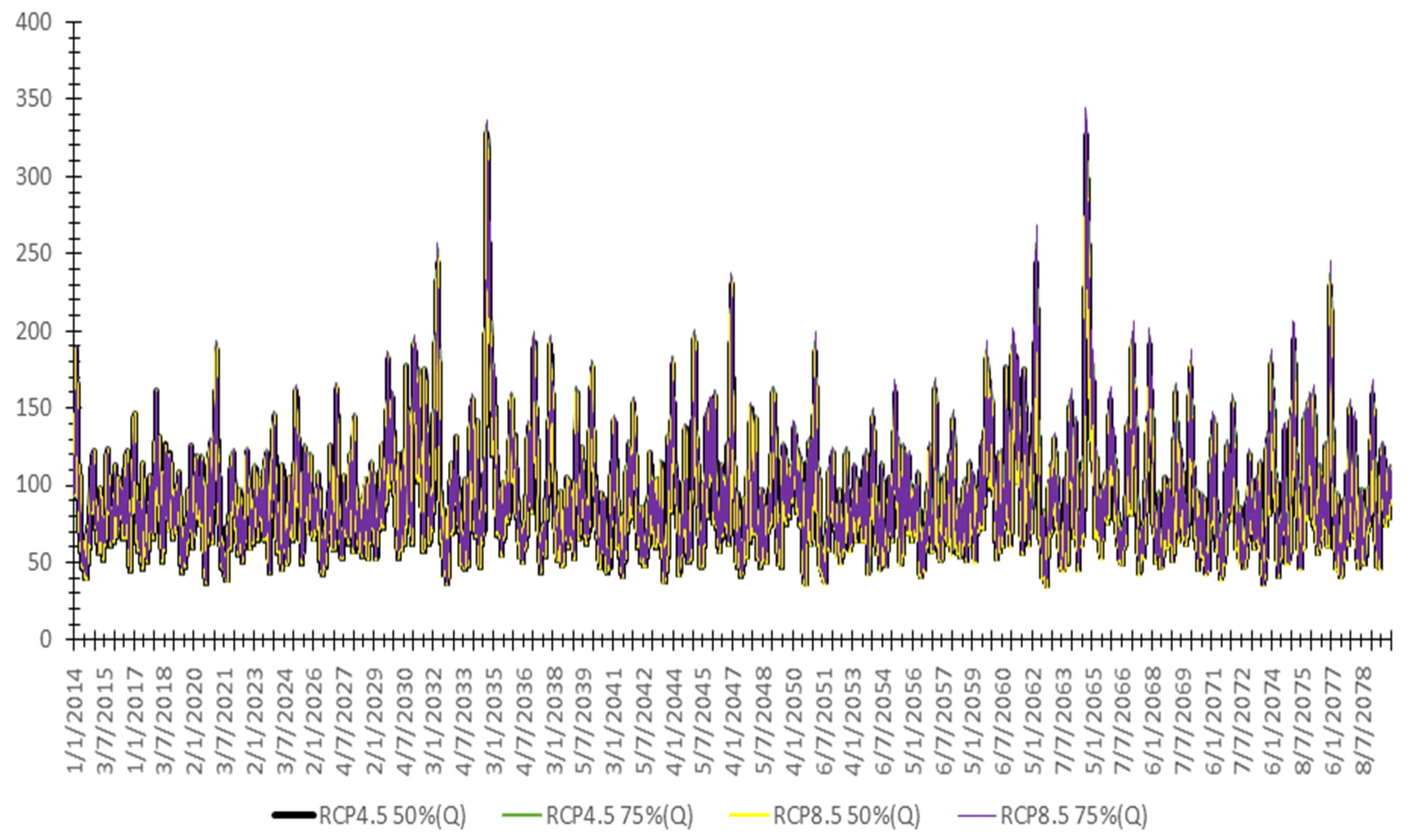
| Parameters | Climatic Scenario (Q(m3)) Prediction | |||
|---|---|---|---|---|
| RCP4.5 50% (Q) | RCP4.5 75% (Q) | RCP8.5 50% (Q) | RCP8.5 75% (Q) | |
| Mean | 89.57 | 90.94 | 88.92 | 91.04 |
| SEMean | 0.200 | 0.209 | 0.203 | 0.217 |
| StDev | 31.12 | 32.46 | 31.48 | 33.67 |
| Variance | 968.93 | 1054.24 | 991.52 | 1133.68 |
| CVariation | 34.75 | 35.70 | 35.41 | 36.98 |
| Q1 | 69.04 | 69.58 | 68.12 | 68.92 |
| Median | 83.14 | 84.06 | 82.48 | 83.87 |
| Q3 | 103.22 | 104.82 | 102.65 | 105.25 |
| IQR | 34.18 | 35.23 | 34.52 | 36.32 |
| TRMean | 86.97 | 88.16 | 86.29 | 88.12 |
| Sum | 21.91 × 10⁵ | 21.92 × 10⁵ | 21.43 × 10⁵ | 21.94 × 10⁵ |
| Minimum | 37.10 | 36.82 | 35.01 | 34.43 |
| Maximum | 327.60 | 336.59 | 328.44 | 344.93 |
| Range | 290.50 | 299.76 | 293.42 | 310.49 |
| SSQ | 21.67 × 10⁷ | 22.47 × 10⁷ | 21.45 × 10⁷ | 22.71 × 10⁷ |
| Skewness | 1.78 | 1.81 | 1.77 | 1.81 |
| Kurtosis | 6.11 | 6.10 | 5.97 | 5.99 |
| MSSD | 59.25 | 63.09 | 59.97 | 66.10 |
| Parameters | Climatic Scenario (WL(m)) Prediction | |||
|---|---|---|---|---|
| RCP4.5 50% (WL) | RCP4.5 75% (WL) | RCP8.5 50% (WL) | RCP8.5 75% (WL) | |
| Mean | 33.278 | 33.277 | 33.281 | 33.280 |
| SEMean | 0.000 | 0.000 | 0.000 | 0.000 |
| StDev | 0.036 | 0.038 | 0.037 | 0.039 |
| Variance | 0.001 | 0.001 | 0.001 | 0.002 |
| CVariation | 0.109 | 0.113 | 0.112 | 0.118 |
| Q1 | 33.259 | 33.258 | 33.261 | 33.260 |
| Median | 33.281 | 33.281 | 33.283 | 33.283 |
| Q3 | 33.305 | 33.305 | 33.308 | 33.309 |
| IQR | 0.046 | 0.047 | 0.048 | 0.049 |
| TRMean | 33.280 | 33.279 | 33.283 | 33.282 |
| Minimum | 33.127 | 33.123 | 33.129 | 33.120 |
| Maximum | 33.381 | 33.383 | 33.388 | 33.392 |
| Range | 0.253 | 0.260 | 0.259 | 0.272 |
| Skewness | −0.775 | −0.810 | −0.753 | −0.806 |
| Kurtosis | 0.672 | 0.759 | 0.604 | 0.733 |
| MSSD | 0.000 | 0.000 | 0.000 | 0.000 |
Publisher’s Note: MDPI stays neutral with regard to jurisdictional claims in published maps and institutional affiliations. |
© 2022 by the authors. Licensee MDPI, Basel, Switzerland. This article is an open access article distributed under the terms and conditions of the Creative Commons Attribution (CC BY) license (https://creativecommons.org/licenses/by/4.0/).
Share and Cite
Gharbia, S.; Riaz, K.; Anton, I.; Makrai, G.; Gill, L.; Creedon, L.; McAfee, M.; Johnston, P.; Pilla, F. Hybrid Data-Driven Models for Hydrological Simulation and Projection on the Catchment Scale. Sustainability 2022, 14, 4037. https://doi.org/10.3390/su14074037
Gharbia S, Riaz K, Anton I, Makrai G, Gill L, Creedon L, McAfee M, Johnston P, Pilla F. Hybrid Data-Driven Models for Hydrological Simulation and Projection on the Catchment Scale. Sustainability. 2022; 14(7):4037. https://doi.org/10.3390/su14074037
Chicago/Turabian StyleGharbia, Salem, Khurram Riaz, Iulia Anton, Gabor Makrai, Laurence Gill, Leo Creedon, Marion McAfee, Paul Johnston, and Francesco Pilla. 2022. "Hybrid Data-Driven Models for Hydrological Simulation and Projection on the Catchment Scale" Sustainability 14, no. 7: 4037. https://doi.org/10.3390/su14074037
APA StyleGharbia, S., Riaz, K., Anton, I., Makrai, G., Gill, L., Creedon, L., McAfee, M., Johnston, P., & Pilla, F. (2022). Hybrid Data-Driven Models for Hydrological Simulation and Projection on the Catchment Scale. Sustainability, 14(7), 4037. https://doi.org/10.3390/su14074037