Article

ELM-Based Non-Singular Fast Terminal Sliding Mode Control Strategy for Vehicle Platoon

1
The Key Laboratory of Road and Traffic Engineering, Ministry of Education, Tongji University, Shanghai 201804, China
2
College of Transportation Engineering, Tongji University, Shanghai 201804, China
*
Author to whom correspondence should be addressed.
Sustainability 2022, 14(7), 4020; https://doi.org/10.3390/su14074020
Submission received: 30 January 2022 / Revised: 21 March 2022 / Accepted: 24 March 2022 / Published: 29 March 2022

Abstract

:
Vehicle platoon is one of the innovations in the automated highway systems, which has the potential to reduce fuel consumption, alleviate traffic congestion and lighten the driver’s burden. How to control the vehicle effectively to ensure the stability of the queue is a challenge. Aiming to overcome the shortcomings of the platoon control method based on traditional sliding mode control, a non-singular terminal sliding mode control method optimized by the extreme learning machine is proposed in this paper. Firstly, the vehicle longitudinal dynamics are derived from the analysis of the forces acting on the vehicle in the longitudinal direction. A constant time headway policy is taken as the spacing policy. The modified non-singular terminal sliding mode control method has outstanding performance, simulation results demonstrate that the following vehicles can rapidly track the trajectory of the leading vehicle in the platoon with less spacing error and guarantee string stability. In this study, several experiments are set up to consider the disturbance and other uncertain practical factors. The performance of the proposed method is superior to the traditional sliding mode control method. Experimental results show that the proposed method can significantly reduce chattering and has good robustness under the circumstances of the disturbance.

1. Introduction

For the past few decades, traffic congestion has become a worldwide problem. The ever-growing traffic demand has overburdened the highway system, and the capacity of the bottleneck sections of the highway is even lower than that of ordinary roads [1,2]. In 1992, the automated highway system (AHS) program was launched, aiming to link the road and the vehicle to maximize driving performance, alleviate traffic congestion, and enhance safety. However, due to the limitation of information and communication technology (ICT), the AHS project has made slow progress since about 2000 [3]. The improvement of wireless communication technology, roadside facilities, various sensors, computer power, and advanced onboard information processing units, brings the hope of solving existing technology bottlenecks [4].
Along with the development of intelligent transportation systems(ITS), vehicle platoon has received a wide range of attention from academia and industry [5,6]. Platoon behavior exists widely in nature. For example, geese on seasonal migration form formations, and ants form formations to carry food. Why do they exhibit such behavior? This is because there are two key skills that animals unconsciously use, namely “information transfer” and “energy-saving” [7]. Does the behavior of these creatures inspire humans? The answer is yes [1,8].
Vehicle platoon is the linking of two or more vehicles in a convoy with tight spacing using wireless communications and sensor technology. The benefits of autonomous platoon control of vehicles are obvious [9]:
  • It reduces the number of drivers and reduces the cost of labor.
  • No driving hazards caused by fatigue driving, which improves safety;
  • Automatic control allows more precise control of output power, thus reducing energy consumption and being more environmentally friendly.
  • Automatic control makes the ability to adjust the spacing more accurate, and reducing the distance can increase the efficiency of the road.
  • For vehicles with the large windward areas, such as trucks, intensive workshop distance control can effectively reduce the power loss caused by wind resistance.
The main contribution of this paper is to design a new multi-vehicle platoon control method, which uses the non-singular fast terminal sliding surface instead of the traditional terminal sliding surface to solve the singularity problem and make the system quickly approach to the steady state. On this basis, the system parameters can be estimated by extreme learning machine neural network, which solves the problem of uncertain or unknown vehicle system parameters and significantly reduces the error. The remainder of this paper is organized as follows: Section 2 primarily analyses the current research status in this field of platoon through the literature in recent years. Section 3 gives mathematical derivation of the vehicle dynamics model. Section 4 is devoted to the vehicle platoon model description and problem formulation. Section 5 contains the analysis of the performances of the verification experiments and the effectiveness of the control method. Section 6 presents a brief conclusion.

2. Related Work/Literature Review

Intelligent vehicle has the characteristics of parameter uncertainty, time delay and highly nonlinear, so its motion control method is the key to realize the autonomous driving of the vehicle. In order to realize longitudinal platoon control, a suitable spacing control model should be established [2].
The core of the vehicle platoon is the vehicle driving controller, which adjusts the speed of the vehicle to maintain a safe distance from the vehicle in front and to keep the fleet at a safe speed for efficient driving. The establishment of the system mathematical model and the design of the controller algorithm are the two most critical parts. Numerous scholars and researchers have made critical contributions to these studies.
In 1953, Pipes from the University of California studied the dynamic characteristics of multi-vehicle formation in a single lane, speculated a “law of separation” to maintain the distance between the front and rear vehicles, and carried out a theoretical study on the dynamic characteristics of the vehicle following action [10]. In the 1960s, some scholars proposed that multiple vehicles could be combined into a string system [11]. They used the optimal control law to design a linear feedback system on which the position and speed of the vehicle could be adjusted. In 1996, Swaroop et al. [12] proposed the evaluation standard of string stability, which became an important theoretical basis for the design of vehicle platoon controller. This theory was a landmark advance. However, due to the limitations of wireless devices, central servers, and various sensor technologies, the formation measurement and information transmission capabilities of early designs are limited. In the past 20 years, the rapid development of vehicle-to-vehicle (V2V), vehicle-to-roadside-units (V2I), vehicle-to-everything (V2X), Internet of Vehicles (IoV) technologies and the progress of communication technology have broadened the design ideas of vehicle formation controller [13,14,15]. More advanced vehicle control strategies are springing up [16,17,18,19,20].
Vehicle platoon control requirements are complex. When the platoon encounter special circumstances or the speed changes, how to maintain the stable spacing error is the key issue [21]. Wireless communication technology and other new technologies have brought many new ideas for formation realization, which can be roughly divided into the following four categories according to the choice of theoretical basis: behavior based method [22,23], artificial potential field method [24,25], model prediction control method [26,27] and leader-follower method. This following will analyze these representative literatures from four directions.
Behavior-based approaches require rational design of basic vehicle driving behavior. Roya et al. [28], based on the offline motion planner system and the online layered control system, proposed a multi-lane formation autonomous navigation architecture. Based on the behavior method, all vehicles in the formation can be constrained and optimized, with no collision trajectory and smooth movement. Chai et al. [29], based on the observation-based event trigger control strategy, proposed a formation time-varying control method for multi-agent systems. This control method allows each individual in the formation to use the current information to update the next action.
As a kind of virtual force method, the basic idea of artificial potential field is to establish different potential fields to control the movement of the vehicle. Li et al. [30] proposed a new formation optimization method. This method was derived from the combination of graph theory and safety potential field theory and was applicable to different vehicle distribution. Yang et al. [31] proposed a car-following model incorporating the artificial potential field theory. This method was used to analyze vehicle following behavior by treating the vehicle as an individual in the charge field. When solving the formation control problem, Nair et al. [32] adopted the artificial potential field to do path planning and proposed a control strategy designed by the improved non-singular terminal sliding mode method.
The core idea of model predictive control is rolling time domain control strategy. In order to deal with unknown disturbances and improve the anti-interference ability of formation system, an improved distributed model prediction method was designed by Liu et al. [33]. The Nash-optimization strategy is used to solve the optimization problem of the model prediction method, which can improve the convergence of the iterative algorithm. In order to overcome the communication delay, Lan et al. [34] proposed a new stability margin judgment method. This method can be used for model predictive control of nonlinear formation systems. The verification experiment showed that each vehicle in the formation only transmits its current acceleration to the adjacent following vehicle, so the information transmission efficiency was very high. Mao et al. [35] proposed an improved collision-free navigation method. The safety zone was taken as the decision constraint and transferred to the input of the model prediction controller after transformation.
Liang et al. [36] developed a position estimator that can provide online position estimates of followers relative to leaders, thus ensuring the stability of the entire formation system. Yang et al. [21] designed a fuzzy PI controller for vehicle safety following control, which can effectively eliminate the influence of information delay in the platoon. Defoort et al. [37] developed a coordinated control scheme based on the leader-following method, and proposed a sliding mode controller that can ensure the gradual adjustment of vehicles to the desired formation effect. Qian et al. [38] and Yuan et al. [39] have combined the observer with the sliding mode method. The difference is that the former uses a nonlinear perturbation observer, while the latter uses an extended state observer. From the experimental results, both of them have achieved good performance in specific experimental scenarios.
Although the existing theoretical research has provided many methods to solve the problem of platoon control, for the actual road traffic environment, the study of vehicle platoon is still difficult. At present, for the random disturbance factors and other external conditions, there are still more studies to be done on the application in various real scenarios, and many difficulties need to be overcome to improve the control strategy of vehicle platoon.

3. Mathematical Derivation of the Vehicle Dynamics Model

In this paper, a schematic diagram of the longitudinal movement of the platoon is shown in Figure 1. All vehicles in the platoon maintain stability through uniform constraint rules, which are comprehensively characterized by factors such as the spacing error and speed of the vehicles. Here, x i ( i = 0 , 1 , 2 , , n ) denotes the position of the ith vehicle. The index number of the vehicle is equal to 0, indicating that the vehicle is the leader of the platoon, namely, the first vehicle in the platoon. Furthermore, x 0 and v 0 stand for the position and velocity of the leading vehicle, respectively. Similarly, x n and v n stand for the position and velocity of the following vehicle n, respectively.

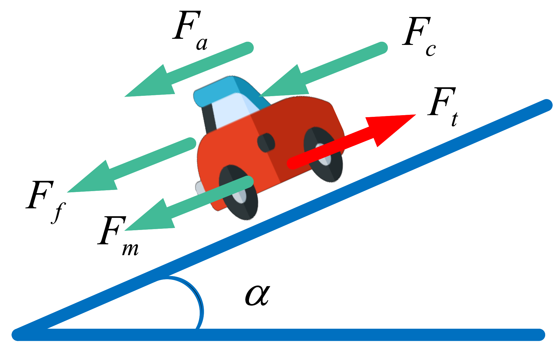
3.1. Single Vehicle Dynamics

A vehicle platoon is composed of a large number of individuals along the driving direction. In order to solve the modeling and control problem of the vehicle platoon, the speed control system of single vehicle could be firstly modeled in straight lane. The beginning of the vehicle model in this paper can be obtained from some vehicle-related textbooks [40,41]. One of the contributions is the vehicle model that can be used for vehicle platoon control completely on the basis of vehicle force analysis, and this model largely reflects the actual situation of vehicles.
For any vehicle in a platoon, without loss of generality, assume that the vehicle travels on a horizontal road surface, the tractive force of the vehicle F t is mainly composed of rolling resistance F f , air resistance F c , mechanical resistance F m and acceleration resistance F a (ignoring the influence of wind speed) [40]. A diagram of longitudinal force on the vehicle is shown in Figure 2.
F t = F f + F c + F m + F a
According to Newton’s second law, the parts on the right side of the equal sign can be further expanded and written as follows:
F t = G f cos α + C D A 21.15 v 2 + K m + δ m d v d t
where δ = 1 + 1 m I w r 2 + 1 m I f i g 2 i 0 2 η T r 2 represents the conversion coefficient of automobile rotating mass. I w , I f , i g , and i 0 denote vehicle inertia, flywheel inertia, main drive ratio, and transmission speed ratio, respectively [41]. For ease of calculation, the Equation (1) is converted to form as follows:
F a = F t F f F c F m
The Equations (2) and (3) can lead to:
δ m i x ¨ i = F t , i G i f cos α C D A 21.15 x ˙ i 2 K m , i
This study is an extension of research based on vehicle dynamics analysis. Based on the force analysis of the single vehicle, an important basis for vehicle platoon control can be established. According to the analysis of the force relation and its derived relation, the design method of the platoon controller can be available.

3.2. Description of Platoon Longitudinal Dynamics

Considering the external disturbance d 1 , i t to the ith vehicle at time t, the Equation (4) can be further derived in the following form:
δ m i x ¨ i = F t , i k f m i g k c x ˙ i 2 K m , i + d 1 , i t
where k f and k c denote coefficient of rolling resistance and coefficient of air resistance, respectively. The relationship of vehicle traction and control signal can be regarded as a first-order nonlinear differential equation:
F ˙ t , i = u i F t , i τ i x ˙ i + d 2 , i t
where u i denotes the controller output of the ith vehicle. τ i x ˙ i represents the instantaneous time constant at x ˙ i . d 2 , i t stands for the internal disturbance of the ith vehicle at time t.
Considering the conversion coefficient of automobile rotating mass usually satisfies 1 < δ < 1.5 , while i g i 0 is very small, δ is a number that goes very close to 1. In order to facilitate calculation, δ is set as 1 in this paper. The simultaneous the Equations (5) and (6), after rearranging, give us:
m i x i + 2 k c x ˙ i x ¨ i d ˙ 1 , i t = 1 τ i x ˙ i u i m i x ¨ i k c x ˙ i 2 K m , i k f m i g + d 1 , i t + d 2 , i t
Tidy up the parts on both sides of the equal sign. We get:
m i x i = 1 τ i x ˙ i u i m i x ¨ i k c x ˙ i 2 K m , i k f m i g + d 1 , i t 2 k c x ˙ i x ¨ i + d ˙ 1 , i t + d 2 , i t = 1 τ i x ˙ i m i x ¨ i + k c x ˙ i 2 + K m , i + k f m i g 2 k c x ˙ i x ¨ i + u i τ i x ˙ i + d 1 , i t τ i x ˙ i + d ˙ 1 , i t + d 2 , i t
The Equation (8) can be rewritten as follows:
x i = 1 m i τ i x ˙ i · u i + f x ˙ i , x ¨ i + 1 m i d 1 , i t τ i x ˙ i + d ˙ 1 , i t + d 2 , i t
where
f x ˙ i , x ¨ i = 1 τ i x ˙ i x ¨ i + k f g + k c x ˙ i 2 + K m , i k c x ˙ i 2 + K m , i m i m i 2 k c m i x ˙ i x ¨ i
x i is actually the same thing as v ¨ i . Based on the Equation (9), we can get
v ¨ i = 1 m i τ i v i · u i + f v i , v ˙ i + 1 m i d 1 , i t τ i v i + d ˙ 1 , i t + d 2 , i t
and
f v i , v ˙ i = 1 τ i v i v ˙ i + k f g + k c v i 2 + K m , i k c v i 2 + K m , i m i m i 2 k c m i v i v ˙ i
The final form of the equation of state can be simplified to
v ¨ i = g v i · u i + f v i , v ˙ i + d ˜ i
where
d ˜ i = 1 m i d 1 , i t τ i v i + d ˙ 1 , i t + d 2 , i t
g v i = 1 m i τ i v i
The vehicle model used for platoon control is completely on the basis of vehicle force analysis. This model largely reflects the actual situation of vehicles. The control effect of each vehicle and its physical characteristics are related. In this paper, the model of the vehicle is as much as possible in accordance with the actual situation.

4. Problem Formulation and Controller Design for Vehicle Platoon

The constant time headway (CTH) control strategy only needs to obtain the state information of the previous vehicle and the current vehicle, which is easy to implement, therefore it is widely used. Based on this control strategy, the complex dynamic characteristics of the platoon can be described by a linear model in this paper.
Time headway and speed act together to determine the workshop distance between two adjacent vehicles. Platoon control can be realized by the error constraint of workshop distance. The workshop distance error between adjacent vehicles in the platoon is defined as follow:
e i = l i 1 + h x ˙ i + x i x i 1
To reduce the computational burden, a simplified configuration of longitudinal movement vehicles in the platoon is necessary. The platoon control of vehicles can be assumed to be described by a second-order nonlinear system as follow:
h x ¨ i + x ˙ i x ˙ i 1 = e ˙ i e ¨ i = h · f v i , v ˙ i + g v i · u i + d ˜ + x ¨ i x ¨ i 1

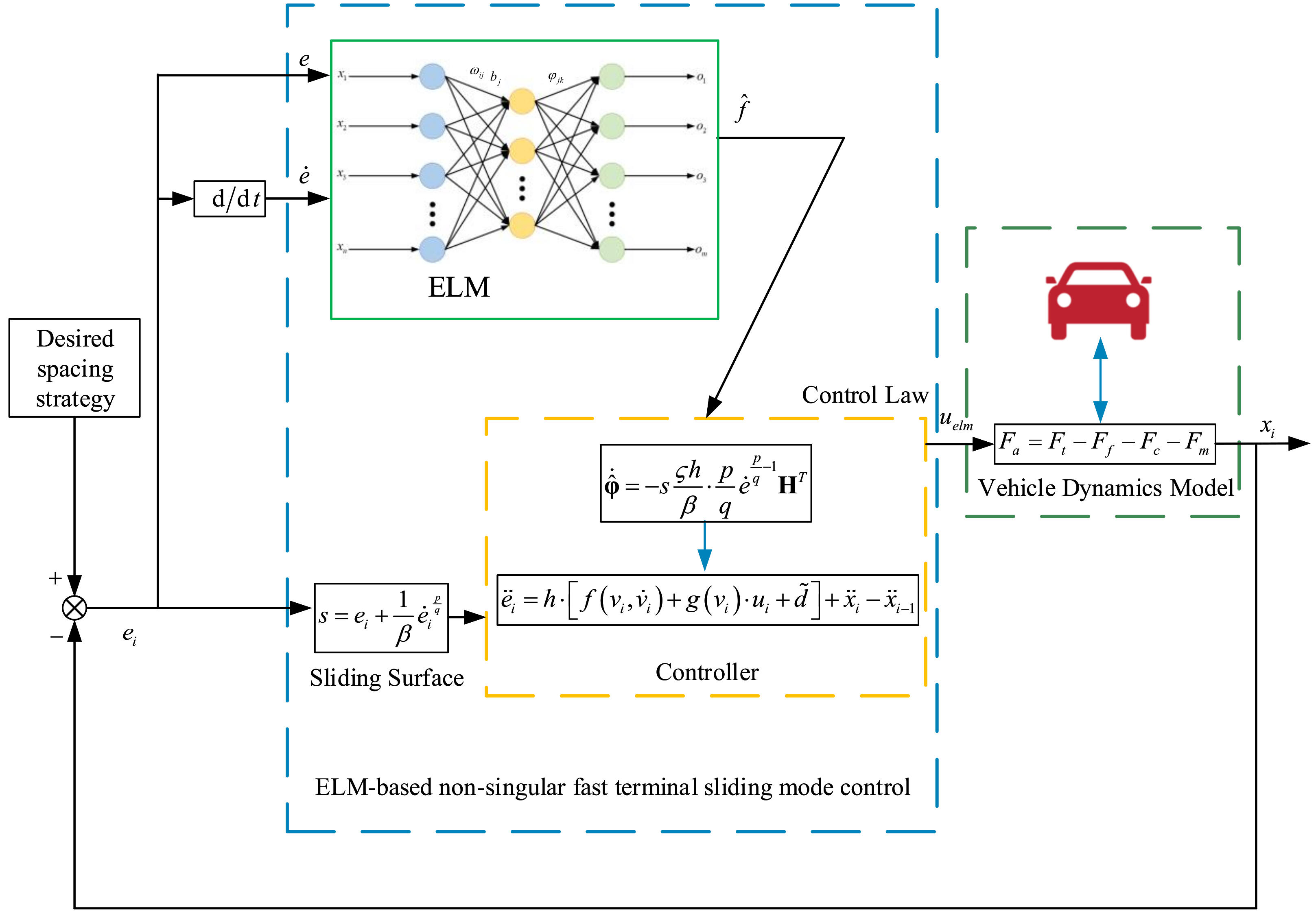
4.1. The Principle of Non-Singular Fast Terminal Sliding Mode Control

Sliding mode control enables the system state trajectory to converge to the sliding mode surface in finite time under the action of the control law and then converge asymptotically to the equilibrium point along the sliding mode surface. However, the asymptotic convergence cannot meet the requirements of vehicle control. The non-singular fast terminal sliding mode control (NFT-SMC) method can improve the convergence speed and control precision by introducing nonlinear parts on this basis so that the system converges in a finite time.
NFT-SMC has relatively fast convergence speed and excellent tracking accuracy. The dynamic performance of NFT-SMC method is better than that of the traditional sliding mode control method, and the singularity problem is avoided. With this control method, the system can converge in a finite time. Sliding mode switching surface function is designed as follow:
s = e i + 1 β e ˙ i p q
NFT-SMC control law is designed as follow:
u i = 1 g v i · f v i , v ˙ i + 1 h · β · q p · e ˙ i 2 p q + D + η · sgn ( s ) + 1 h · x ¨ i x ¨ i 1
The Lyapunov function is chosen as:
V = 1 2 s 2
Consequently,
V ˙ = s s ˙
Theorem 1.
Let d ˜ satisfies the hypothesis of d ˜ D , and 1 < p q < 2 , p > q , β > 0 , η > 0 , where p and q are both positive odd numbers. Then, for nonlinear system model (17), the stability of the closed-loop system can be guaranteed by adopting the sliding mode surface function (18) and the control law (19), and the tracking error can converge to 0 asymptotically in a finite time.
Proof of Theorem 1. 
The proof of stability is based on Lyapunov’s theorem. We conclude from the Equation (18) that as follows:
s ˙ = e ˙ + 1 β · p q e ˙ p q 1 · e ¨
= e ˙ + 1 β · p q e ˙ p q 1 · h · f v i , v ˙ i + g v i · u i + d ˜ + x ¨ i x ¨ i 1
= e ˙ + 1 β · p q e ˙ p q 1 · h · f v , v ˙ g v · h g v · f v , v ˙
+ 1 h · β · q p · e ˙ i 2 p q + D + η · sgn ( s ) + 1 h · x ¨ i x ¨ i 1 + d ˜ + x ¨ i x ¨ i 1
= h β · p q e ˙ p q 1 D + η · sgn ( s ) + d ˜
Hence that,
V ˙ = h β · p q e ˙ p q 1 s · d ˜ D + η · sgn ( s )
h β · p q e ˙ p q 1 · η · s < 0
The proof is going to be discussed in two cases. Because 1 < p q < 2 , p > q , β > 0 , when e ˙ 0 is satisfied, this clearly forces V ˙ 0 . According to LaSalle invariant principle, we have t , s 0 , namely t , e 0 . When e ˙ = 0 is satisfied, the system can approach 0 in a finite time.
The above finishes the proof. □
In NFT-SMC, the gain of the robust item is set to be slightly larger than the upper bound of the disturbance to compensate for the influence caused by the unknown disturbance, to ensure the stability and trajectory tracking performance of the system.

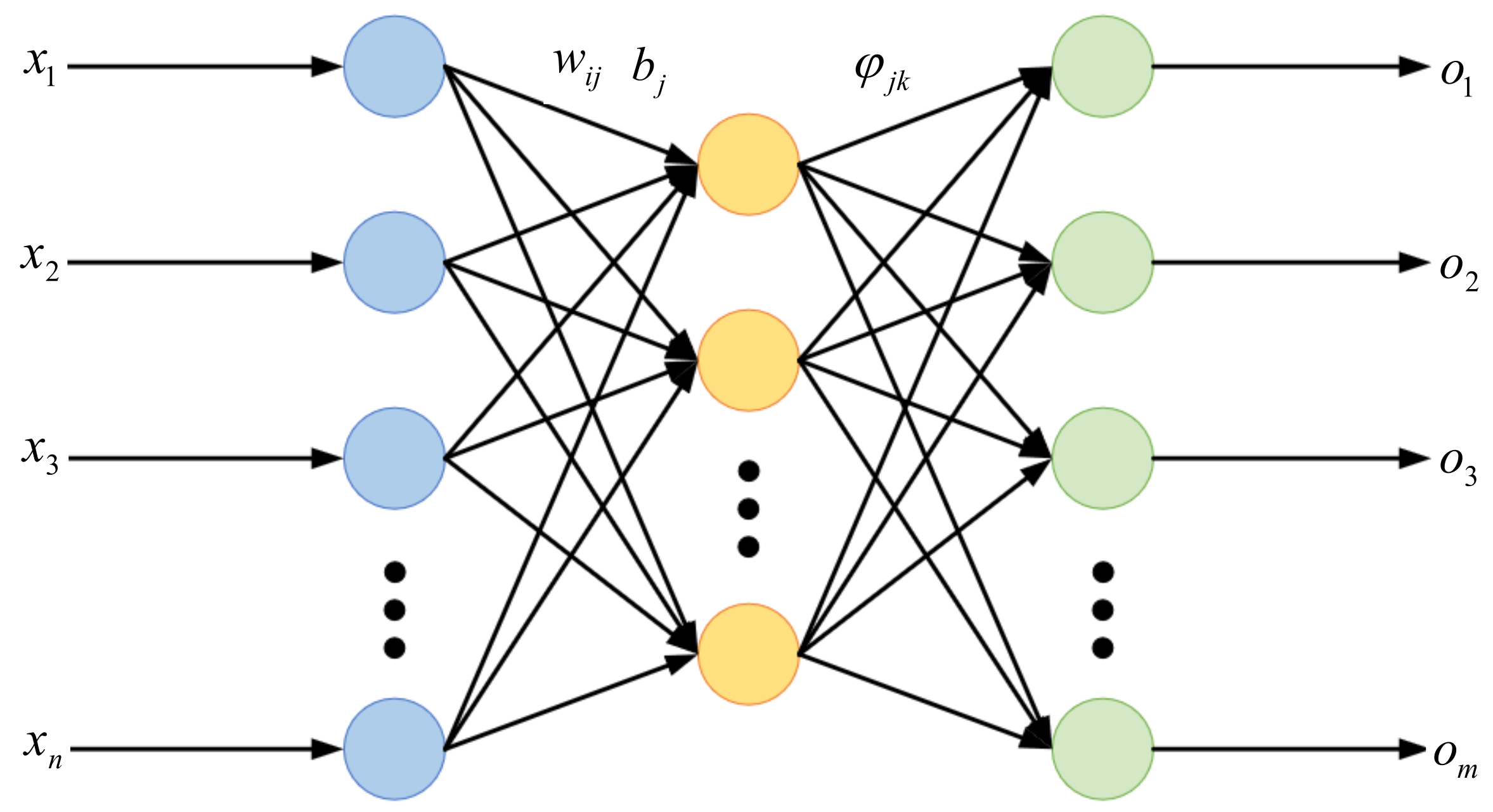
4.2. Extreme Learning Machine Optimized NFT-SMC

The quality of the control algorithm in the controller is directly related to the performance of the vehicle. In the field of vehicle control, low latency and high accuracy are required for autonomous vehicles. Generally, decimeter-level positioning and centimeter-level positioning are the requirements of self-driving vehicle for highway operation and residential streets operation, respectively [42,43]. In practice, it is difficult to establish an accurate platoon control model for the multi-vehicle systems due to uncertain parameters and external disturbance. Furthermore, due to the chattering phenomenon, the control performance of SMC is inhibited.
To reduce chattering and improve self-learning ability, an extreme learning machine (ELM) modified terminal sliding mode control for vehicular platoon is proposed in this paper.
As a kind of neural network, ELM can approximate the uncertain part of control parameters and has certain reasoning abilities. The most remarkable feature is the speed of calculation.
Since f v , v ˙ in the control law (19) is unknown, the precision of the control depends on the precision of parameter identification. Neural networks can realize the adaptive approximation of unknown parts. Motivated by this construction, the extreme learning machine method is introduced in this paper. Extreme learning machine can maintain fast learning ability while maintaining good generalization performance. For a deeper discussion of the ELM, we refer the reader to [44,45]. The schematic diagram of the ELM neural network is shown in Figure 3.
Concretely,
o j = o 1 j o 2 j o m j = i = 1 l φ i 1 g w i · x j + b i i = 1 l φ i 2 g w i · x j + b i i = 1 l φ i m g w i · x j + b i
where j = 1 , 2 , , N , w i = w i 1 , w i 2 , , w i n , x j = x 1 j , x 2 j , , x n j T .
We can arrange the Equation (24) to get:
H φ = O T φ T H T = O
where H denotes hidden layer output matrix.
H = g w 1 · x 1 + b 1 g w 2 · x 1 + b 2 g w l · x 1 + b l g w 1 · x 2 + b 1 g w 2 · x 2 + b 2 g w l · x 2 + b l g w 1 · x N + b 1 g w 2 · x N + b 2 g w l · x N + b l
The process of training the neural network is the process of adjusting the connection coefficient weight β . The ultimate goal is to get a parameter configuration that minimizes error.
min φ H φ O T
The framework overview of extreme learning machine optimized NFT-SMC is shown in Figure 4. The combination of the error and the derivative of the error is taken as the input of the neural network:
y = [ e , e ˙ ]
f ^ is an estimate of f, and it can be written as:
f ^ = φ ^ T H T
where φ ^ denotes the estimate of coefficient weight φ . The actual value of f is:
f = φ T H T + ε ( y )
where φ denotes the best estimate of coefficient weight φ . ε ( y ) represents the approximation error of the neural network. ε ( y ) ζ . ζ is a positive value. By the above, we can obtain:
f ˜ = f f ^ = φ T H T φ ^ T H T + ε ( y ) = φ φ ^ T H T + ε ( y ) = φ ˜ T H T + ε ( y )
where φ ^ φ = φ ˜ φ ^ ˙ = φ ˜ ˙ . f = φ ˜ T H T + φ ^ T H T + ε ( y ) .
The modified control law is designed as follow:
u e l m = 1 g v i · f ^ v i , v ˙ i + 1 h · β · q p · e ˙ i 2 p q + D + η · sgn ( s ) + 1 h · x ¨ i x ¨ i 1
Theorem 2.
For nonlinear system model (17), the stability of the closed-loop system can be guaranteed by adopting the sliding mode surface function 18, the adaptive control law (35) and the control law (32), and the tracking error (16) can converge to 0 asymptotically in a finite time.
Proof of Theorem 2. 
The proof of stability is similar to the above. The modified Lyapunov function is chosen as:
V = 1 2 s 2 + 1 2 ς φ ˜ T φ ˜ , ς > 0
Therefore,
V ˙ = s s ˙ + 1 ς φ ˜ T φ ˜ ˙
= s s ˙ + 1 ς φ ˜ T φ ^ ˙ = s e ˙ + 1 β · p q e ˙ p q 1 · e ¨ + 1 ς φ ˜ T φ ^ ˙ = s e ˙ + 1 β · p q e ˙ p q 1 · h · f · + g v · u e l m + d ˜ + x ¨ i x ¨ i 1 + 1 ς φ ˜ T φ ^ ˙ = s e ˙ + 1 β · p q e ˙ p q 1 · h f ˜ · + h f ^ · g v · h g v · f ^ · + 1 h · β · q p · e ˙ i 2 p q + D + η · sgn ( s ) + 1 h · x ¨ i x ¨ i 1 + d ˜ + x ¨ i x ¨ i 1 φ ˜ T φ ^ ˙ = s h β · p q e ˙ p q 1 φ ˜ T H T + ε ( y ) D + η · sgn ( s ) + d ˜ φ ˜ T φ ^ ˙ = h β · p q e ˙ p q 1 s ε ( y ) + s d ˜ D + η · s + s h β · p q e ˙ p q 1 φ ˜ T H T + 1 ς φ ˜ T φ ^ ˙ = h β · p q e ˙ p q 1 s ε ( y ) + s d ˜ D + η · s + φ ˜ T ( s h β · p q e ˙ p q 1 H T + 1 ς φ ^ ˙ )
Choose ζ = η ε N ( ε N > 0 ) , the adaptive control law is adopted as follow
φ ^ ˙ = s ς h β · p q e ˙ p q 1 H T
Hence,
V ˙ h β · p q e ˙ p q 1 s ε ( y ) η · s
ε ( y ) ζ , V ˙ 0
Similarly, we have t , s 0 , namely t , e 0 .
The above finishes the proof. □
The controller designed in this paper is deeply connected with ELM, and various external factors faced by the vehicle are considered more comprehensively during model establishment. In addition to the mathematical proof, the algorithm simulation also verifies the effectiveness of the proposed method.

5. Experiments

5.1. Experimental Parameter Configuration

To demonstrate the effectiveness of the proposed elm-based non-singular fast terminal sliding mode control method, this study used the Simulink in MATLAB (MathWorks, 2020a) to construct the simulation experiment environment of the vehicle platoon. The controller design method proposed in this paper mainly has two control objectives. The first objective is to guarantee the following vehicles to maintain the desired time headway with the preceding vehicle. The second goal is to ensure the string stability of the whole platoon.
Simulation experiments in the following are designed to verify the effectiveness of the proposed method. Gently controlling input can effectively avoid frequent acceleration and deceleration operation, extend the service life of the vehicle actuator, reduce energy consumption and improve ride comfort.
In this experiment, the platoon control system is built under a Simulink environment. Specifically, the vehicle dynamics simulation environment is configured and the vehicle mathematical model is established. Moreover, the controller of the following vehicles are also included in the Simulink environment.
Scenario A and Scenario B fully investigate the effectiveness and adaptability of the method proposed in this study. It is worth mentioning that several periods are set in the experiment, and the desired velocity of the platoon is different in each period. These speed control process include acceleration, deceleration, abrupt deceleration, cyclical acceleration and deceleration, and constant speed. Comparative experiments of different methods are placed at the end. The main parameters in the controller are set in Table 1.

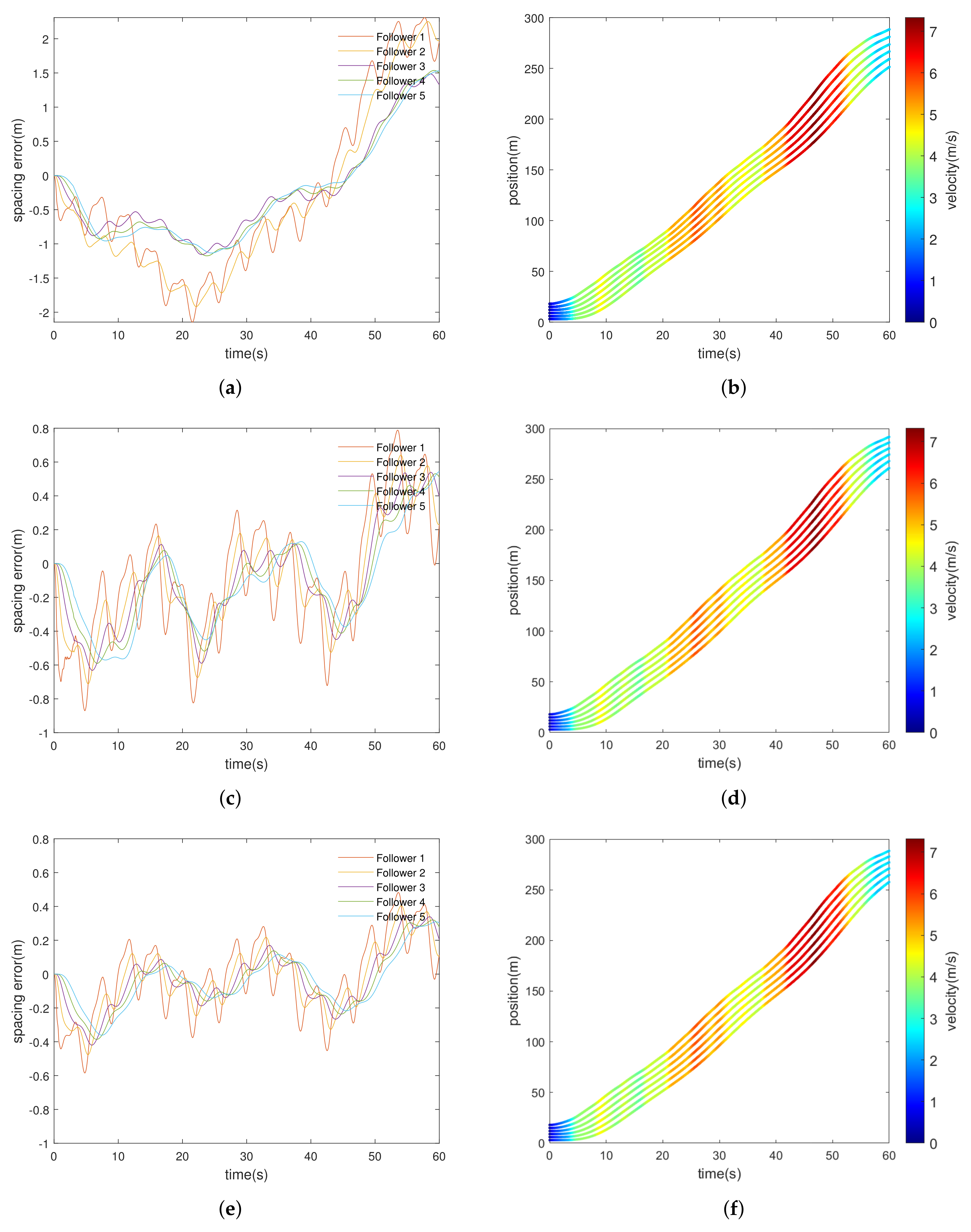
5.2. Simulation Experiment and Result Analysis

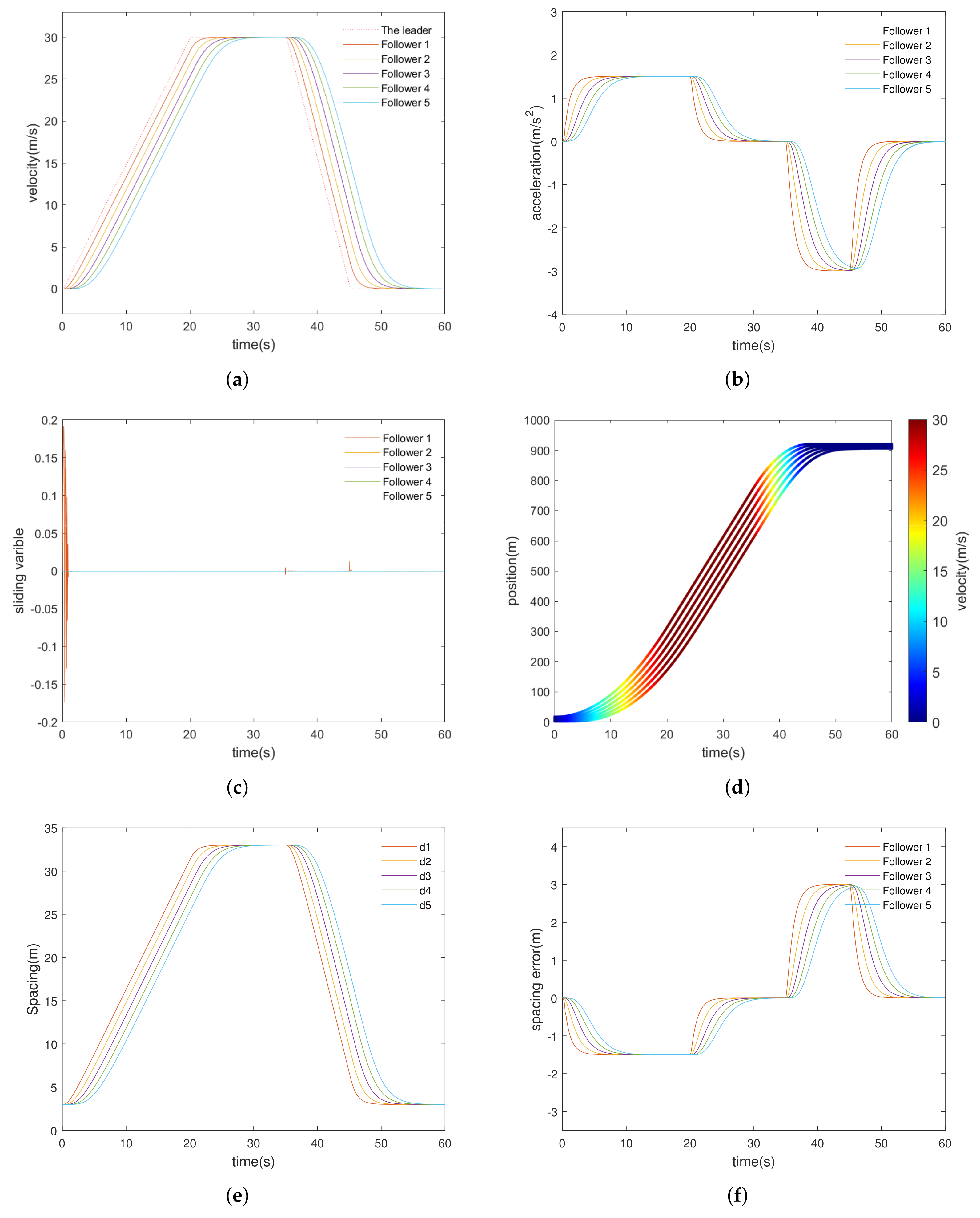
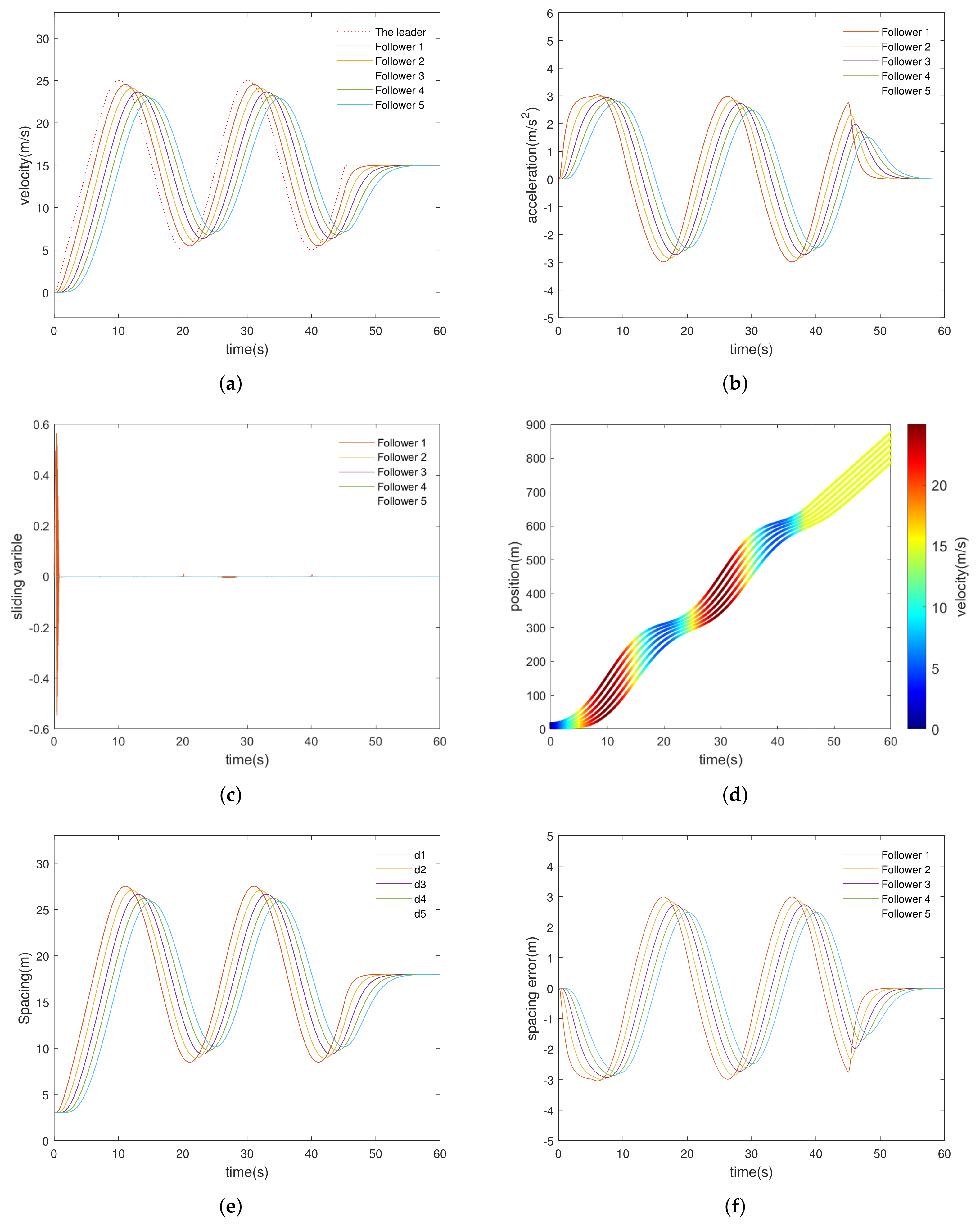
5.2.1. Experiment with Different Types of Scenes

  • Scenario A:
Scenario A describes a typical driving scene: acceleration, steady speed, deceleration. The process can be divided into three stages, firstly accelerating for 20 s to a speed of 30 m/s, then holding speed for 15 s, and finally decelerating to a stop within 10 s. The speed of the lead vehicle is controlled according to the Equation (37).
In this study, a platoon of one leader and N = 5 following vehicles has been simulated to verify the effectiveness of the method presented. The time headway is set as 1 s.
v 0 = 1.5 t m / s , 0 t < 20 s 30 m / s , 20 s t < 35 s 30 3 ( t 35 ) m / s , 35 s t < 45 s 0 m / s , 45 s t < 60 s
Figure 5 is the response of the vehicle platoon based on the proposed method in Scenario A. This study uses six subgraphs to demonstrate the performance of the vehicle platoon in the total simulation period more comprehensively.
Figure 5a shows that each vehicle tracks the speed profile of the preceding vehicle very well, thus achieving good tracking of the lead vehicle. Namely, the following vehicle achieves the goal of keeping the speed of the following vehicle consistent with the speed of the leading vehicle, and the error is close to 0 when the vehicle speed reaches the steady-state. The adjustment time can be controlled within 10 s. Figure 5b describes the acceleration curve of each vehicle. Figure 5c shows the change of the sliding variable. Figure 5d is a schematic diagram of the position changes of each vehicle, which shows the good driving performance of the platoon, no collision occurred, and all vehicles are driving safely. Figure 5e reflects the distance between neighboring vehicles. This experiment uses the CTH strategy. It can be seen that as the speed of the vehicle increases, the distance between vehicles gradually increases. Figure 5f shows the spacing error of the vehicles in the platoon.
During the whole acceleration process, the position and the velocity of each vehicle are controlled stably. No collision occurred between any vehicles. In general, the method presented in this paper performs well in pure acceleration and deceleration, whether from the point of view of safety, stability, or comfort.
  • Scenario B:
To make the simulation scene close to reality, a cyclic acceleration and deceleration condition is designed in Scenario B. This scenario describes a typical vehicle platoon operation: cyclic acceleration and deceleration. The process can be broken down into three stages. Firstly, it takes five seconds to accelerate to a speed of 15 m/s. Then it cycles between acceleration and deceleration for 40 s. Finally, it takes 15 s to drive at a constant speed of 15 m/s. The speed of the leading vehicle is controlled according to the Equation (38). As in Scenario A, there are a total of 5 following vehicles in this experiment. The time headway is also be set to 1 s.
v 0 = 3 t m / s , 0 t < 5 s 15 + 10 sin ( 0 . 1 π ( t 5 ) ) m / s , 5 s t < 45 s 15 m / s , 45 s t < 60 s
Figure 6 is the response of the vehicle platoon control system in Scenario B. From the figure, we can observe the changing process of each car in different stages of time. Taking acceleration as an example, we can observe that the closer the position is to the leading vehicle, the faster the response of acceleration changes.
The cyclic acceleration and deceleration experiment requires the high continuous switching ability of the control system. From the Figure 6a, we can see that the velocity follows well and the adjustment process is very smooth. The transition time to stability is about 10 s. Figure 6b shows that there is no obvious abrupt change in the acceleration and braking stage, and the following car keeps a good tracking effect on the leading vehicle. Figure 6c,d visualizes the change of the sliding variable and the positions of the vehicles, respectively. The results reflect control law can maintain the intervehicle distance well. Figure 6e,f reveal spacing and the spacing error, respectively. Any vehicle in the platoon can follow at the desired speed guarantee the spacing error converges to 0, fastly.

5.2.2. Comparison Experiment

In this part, a group of comparative experiments is carried out for sliding mode control, non-singular fast terminal sliding mode control, and the method proposed in this paper. The speed of the leading vehicle is controlled according to the Equation (39). To be close to the actual speed curve of the leading vehicle, some degree of random disturbance d = 0.1 sin ( 0.1 t ) + 0.2 cos ( 0.2 t ) and periodic disturbance 0.2 r a n d ( 1 ) are added, respectively.
v 0 = 1.2 sin ( 0.15 t ) + 0.25 sin ( 0.2 t ) + 6 sin ( 0.045 t ) + sin ( 0.3 t ) + 0.3 sin ( 1.5 t ) + 0.1 sin ( 3 t ) , 0 s t 60 s
The vehicle platoon system driven by different control methods is validated at the same CTH h value. Comparative experimental results are shown in Figure 7.
Figure 7a,b is the spacing error curve and the position-velocity diagram based on the traditional sliding mode control method. It can be seen from the figure that the maximum spacing error reaches 2.2 m. The spacing error of this method is far from ideal. Compared with other control methods, the speed tracking profile depicts it has the largest delay and converges to the ideal speed curve at the latest. It can be seen that the control effect of the traditional SMC method has obvious defects in the face of harsh scenes such as rapid speed switching. The effect in the figure proves the above analysis.
Figure 7c,d reflect the spacing error of the platoon and the position-velocity relationship based on the non-singular fast terminal sliding mode control method. As shown in the figure, the tracking effect of the spacing is better than that of the traditional sliding mode control method. The convergence speed of spacing error is improved, and the tracking error of the spacing is controlled with the range of 0 to 0.84 m. The vehicle speed tracking delay decreases. Furthermore, the vehicle position tracking performance has been improved.
Figure 7e,f show the spacing error effect and the position-velocity diagram obtained by the ELM-based non-singular fast terminal sliding mode control strategy. It can be seen that compared with the above two methods, the control effect of the proposed method on the CTH strategy shows superiority, and the error is controlled between 0 and 0.6 m. In addition, the spacing error decreases successively from the pilot car to the last following car in the queue, indicating that the platoon shows good stability. The tracking effect of vehicle position track and speed track is very ideal. It is shown that the proposed strategy has a good implementation effect of robust control over system parameter uncertainty and external disturbance.
In summary, the control method proposed in this paper has fast convergence speed, high control accuracy, and strong robustness, and can well track the speed of the leading vehicle with large or continuous small changes. The proposed control strategy cannot only make the tracking error converge to the equilibrium point in ideal time but also has strong robustness.
Under the control of the method in this paper, the stability of the system is the best of the three strategies. Furthermore, there is no abnormal mutation in the acceleration of each vehicle. The amplitude decreases successively with the number of vehicles, and the transfer control strength decreases gradually. Based on ELM networks estimation, the platoon control system can effectively reduce the dependence on system dynamics, improve the anti-interference ability of the system, and significantly reduce the calculation time to improve the response speed of the system. Simulation results reflect the effectiveness and superiority of the proposed control scheme.

6. Conclusions

This study mainly focuses on platoon control. To overcome various problems encountered by vehicle platoon, a fast non-singular terminal sliding mode control method optimized by an extreme learning machine is designed in this paper. The vehicle longitudinal dynamics model is derived and the constant time headway policy is established. The control law of the following vehicle is derived, and the stability of the control system is proved based on the Lyapunov theory. Based on reasonable parameter configuration, two typical working conditions are constructed. The performance of the control system is analyzed by Simulink simulation, and good dynamic response and satisfactory tracking accuracy can be obtained. Finally, a comparative experiment between the proposed method and the traditional SMC and NFT-SMC is given. The control method solves the singular problem and makes the controller system approach to steady-state quickly. Meanwhile, it solves the problem of uncertain or unknown parameters and significantly reduces the error. By using our proposed control method, the following vehicles can quickly approach the ideal spacing and keep stable when the speed mutation occurs. Experimental results show that the proposed method has good robustness, which proves the effectiveness and superiority of the proposed method on vehicle platoon.

Author Contributions

Conceptualization, C.W.; modeling, simulation, and validation, C.W.; writing, original draft preparation, C.W.; supervision and critical review, Y.D. All authors have read and agreed to the published version of the manuscript.

Funding

This research was funded by Shanghai Municipal Education Commission, major Natural Science Project of Scientific Research and Innovation Program (No. 2021-01-07-00-07-E00092).

Informed Consent Statement

Not applicable.

Data Availability Statement

Not applicable.

Conflicts of Interest

The authors declare no conflict of interest.

References

  1. Beaver, L.; Malikopoulos, A. Constraint-Driven Optimal Control of Multiagent Systems: A Highway Platooning Case Study. IEEE Control Syst. Lett. 2021, 6, 1754–1759. [Google Scholar] [CrossRef]
  2. Wang, Z.; Wu, G.; Barth, M. A Review on Cooperative Adaptive Cruise Control (CACC) Systems: Architectures, Controls, and Applications. In Proceedings of the 2018 21st International Conference on Intelligent Transportation Systems (ITSC), Maui, HI, USA, 4–7 November 2018; pp. 2884–2891. [Google Scholar] [CrossRef] [Green Version]
  3. Lakshmi, D.; Bart, D.; Hans, H. Optimal routing for automated highway systems. Transp. Res. Part C Emerg. Technol. 2013, 30, 1–22. [Google Scholar] [CrossRef]
  4. Chen, X.; Chen, H.; Yang, Y.; Wu, H.; Zhang, W.; Zhao, J.; Xiong, Y. Traffic flow prediction by an ensemble framework with data denoising and deep learning model. Phys. A Stat. Mech. Appl. 2021, 565, 125574. [Google Scholar] [CrossRef]
  5. Adil, A.; Anjan, R.; James, W.; Jim, M. Adapting time headway in cooperative adaptive cruise control to network reliability. IEEE Trans. Veh. Technol. 2021, 70, 12691–12702. [Google Scholar] [CrossRef]
  6. Roh, C.; Jeon, H.; Son, B. Do heavy vehicles always have a negative effect on traffic flow? Appl. Sci. 2021, 11, 5520. [Google Scholar] [CrossRef]
  7. Mirzaeinia, A.; Heppner, F.; Hassanalian, M. An analytical study on leader and follower switching in V-shaped Canada Goose flocks for energy management purposes. Swarm Intell. 2020, 14, 117–141. [Google Scholar] [CrossRef]
  8. Gungor, O.; She, R.; Al-Qadi, I.; Ouyang, Y. One for all: Decentralized optimization of lateral position of autonomous trucks in a platoon to improve roadway infrastructure sustainability. Transp. Res. Part C Emerg. Technol. 2020, 2020, 102783. [Google Scholar] [CrossRef]
  9. Keely, V. Distributed Cooperative Control of Heterogeneous Multi-Vehicle Platoons. Master’s Thesis, University of Rhode Island, South Kingstown, RI, USA, 2017. [Google Scholar] [CrossRef]
  10. Pipes, L. An operational analysis of traffic dynamics. J. Appl. Phys. 1953, 24, 274–281. [Google Scholar] [CrossRef]
  11. Levine, W.; Athans, M. On the optimal error regulation of a string of moving vehicles. IEEE Trans. Autom. Control 1966, 11, 355–361. [Google Scholar] [CrossRef]
  12. Swaroop, D.; Hedrick, J.K. String stability of interconnected systems. IEEE Trans. Autom. Control 1996, 41, 349–357. [Google Scholar] [CrossRef]
  13. Prakash, R.; Manivannan, P.V. Simplified node decomposition and platoon head selection: A novel algorithm for node decomposition in vehicular ad hoc networks. Artif. Life Robot. 2017, 22, 44–50. [Google Scholar] [CrossRef]
  14. Huang, C.M.; Lin, T.H.; Tseng, K.C. Bandwidth Aggregating over VANET Using the On-Demand Member-Centric Routing Protocol (OMR). In Proceedings of the 2012 12th International Symposium on Pervasive Systems, Algorithms and Networks, San Marcos, TX, USA, 13–15 December 2012; Volume 22, pp. 89–95. [Google Scholar] [CrossRef]
  15. McAree, O.; Veres, S.M. Lateral control of vehicle platoons with on-board sensing and Inter-Vehicle Communication. In Proceedings of the European Control Conference (ECC), Aalborg, Denmark, 19 June–1 July 2016; pp. 2465–2470. [Google Scholar] [CrossRef] [Green Version]
  16. Wang, H.X.; Liu, T.T.; Kim, B.; Lin, C.W.; Shiraishi, S.; Xie, J.; Han, Z. Architectural Design Alternatives Based on Cloud/Edge/Fog Computing for Connected Vehicles. IEEE Commun. Surv. Tutorials 2020, 22, 2349–2377. [Google Scholar] [CrossRef]
  17. Pourghebleh, B.; Navimipour, N.J. Towards efficient data collection mechanisms in the vehicular ad hoc networks. Int. J. Commun. Syst. 2019, 32, e3893. [Google Scholar] [CrossRef]
  18. Peng, H.X.; Liang, L.; Shen, X.M.; Li, G.Y. Vehicular Communications: A Network Layer Perspective. IEEE Trans. Veh. Technol. 2019, 68, 1064–1078. [Google Scholar] [CrossRef] [Green Version]
  19. Skoufas, K.; Spyrou, E.D.; Mitrakos, D. Low Cost V2X Traffic Lights and Vehicles Communication Solution for Dynamic Routing. In Proceedings of the 8th International Conference on Telecommunications and Remote sensing (ICTRS 2019), Rhodes, Greece, 16–17 September 2019; pp. 56–65. [Google Scholar] [CrossRef]
  20. Vasebi, S.; Hayeri, Y.M. Collective Driving to Mitigate Climate Change: Collective-Adaptive Cruise Control. Sustainability 2021, 13, 8943. [Google Scholar] [CrossRef]
  21. Yang, L.; Sun, D.; Xie, F.; Zhu, J. Study of autonomous platoon vehicle longitudinal modeling. In Proceedings of the IET International Conference on Intelligent and Connected Vehicles(ICV 2016), Chongqing, China, 22–26 September 2016; pp. 1–10. [Google Scholar] [CrossRef]
  22. Lee, G.; Chwa, D. Decentralized behavior-based formation control of multiple robots considering obstacle avoidance. Intell. Serv. Robot. 2017, 11, 127–138. [Google Scholar] [CrossRef]
  23. Balch, T.; Arkin, R.C. Behavior-based formation control for multirobot teams. IEEE Trans. Robot. Autom. 1998, 14, 926–939. [Google Scholar] [CrossRef] [Green Version]
  24. Rasekhipour, Y.; Khajepour, A.; Chen, S.K.; Litkouhi, B. A Potential Field-Based Model Predictive Path-Planning Controller for Autonomous Road Vehicles. IEEE Trans. Intell. Transp. Syst. 2017, 18, 1255–1267. [Google Scholar] [CrossRef]
  25. Huang, Y.J.; Ding, H.T.; Zhang, Y.B.; Wang, H.; Cao, D.P.; Xu, N.; Hu, C. A Motion Planning and Tracking Framework for Autonomous Vehicles Based on Artificial Potential Field Elaborated Resistance Network Approach. IEEE Trans. Ind. Electron. 2020, 67, 1376–1386. [Google Scholar] [CrossRef]
  26. Li, L.H.; Gan, J.; Qu, X.; Lu, W.Q.; Mao, P.P.; Ran, B. A Dynamic Control Method for Cavs Platoon Based on the MPC Framework and Safety Potential Field Model. KSCE J. Civ. Eng. 2021, 25, 1874–1886. [Google Scholar] [CrossRef]
  27. Hong, C.H.; Shan, H.G.; Song, M.Y.; Zhuang, W.H.; Xiang, Z.Y.; Wu, Y.X.; Yu, X.L. A Joint Design of Platoon Communication and Control Based on LTE-V2V. IEEE Trans. Veh. Technol. 2020, 69, 15893–15907. [Google Scholar] [CrossRef]
  28. Firoozi, R.; Zhang, X.; Borrelli, F. Formation and reconfiguration of tight multi-lane platoons. Control Eng. Pract. 2021, 108, 104714–104726. [Google Scholar] [CrossRef]
  29. Chai, X.F.; Liu, J.; Yu, Y.; Sun, C.Y. Observer-based self-triggered control for time-varying formation of multi-agent systems. Sci. China Inf. Sci. 2021, 64, 132205. [Google Scholar] [CrossRef]
  30. Li, L.H.; Gan, J.; Qu, X.; Mao, P.P.; Yi, Z.W.; Ran, B. A Novel Graph and Safety Potential Field Theory-Based Vehicle Platoon Formation and Optimization Method. Appl. Sci. 2021, 11, 958. [Google Scholar] [CrossRef]
  31. Yang, Z.S.; Yu, Y.; Yu, D.X.; Zhou, H.X.; Mo X, L. APF-Based Car Following Behavior Considering Lateral Distance. Adv. Mech. Eng. 2013, 5, 207104. [Google Scholar] [CrossRef]
  32. Nair, R.R.; Karki, H.; Shukla, A.; Behera, L.; Jamshidi, M. Fault-Tolerant Formation Control of Nonholonomic Robots Using Fast Adaptive Gain Nonsingular Terminal Sliding Mode Control. IEEE Trans. Syst. Man-Cybern.-Syst. 2019, 13, 1006–1017. [Google Scholar] [CrossRef]
  33. Liu, A.D.; Zhang, W.A.; Yu, L.; Yan, H.C.; Zhang, R.C. Formation Control of Multiple Mobile Robots Incorporating an Extended State Observer and Distributed Model Predictive Approach. IEEE Trans. Syst. Man-Cybern.-Syst. 2020, 50, 4587–4597. [Google Scholar] [CrossRef]
  34. Lan, J.L.; Zhao, D.Z. Min-Max Model Predictive Vehicle Platooning With Communication Delay. IEEE Trans. Veh. Technol. 2020, 69, 12570–12584. [Google Scholar] [CrossRef]
  35. Mao, R.; Gao, H.; Guo, L. A Novel Collision-Free Navigation Approach for Multiple Nonholonomic Robots Based on ORCA and Linear MPC. Math. Probl. Eng. 2020, 4183427. [Google Scholar] [CrossRef]
  36. Liang, X.W.; Liu, Y.H.; Wang, H.S.; Chen, W.D.; Xing, K.X.; Liu, T. Leader-Following Formation Tracking Control of Mobile Robots Without Direct Position Measurements. IEEE Trans. Autom. Control 2016, 61, 4131–4137. [Google Scholar] [CrossRef]
  37. Defoort, M.; Floquet, T.; Kokosy, A.; Perruquetti, W. Sliding-Mode Formation Control for Cooperative Autonomous Mobile Robots. IEEE Trans. Ind. Electron. 2008, 55, 3944–3953. [Google Scholar] [CrossRef] [Green Version]
  38. Qian, D.W.; Tong, S.W.; Li, C.D. Leader-Following Formation Control of Multiple Robots with Uncertainties through Sliding Mode and Nonlinear Disturbance Observer. Etri J. 2016, 38, 1008–1018. [Google Scholar] [CrossRef]
  39. Yuan, Z.Y.; Tian, Y.X.; Yin, Y.F.; Wang, S.Y.; Liu, J.X.; Wu, L.G. Trajectory tracking control of a four mecanum wheeled mobile platform: An extended state observer-based sliding mode approach. IET Control Theory Appl. 2020, 14, 415–426. [Google Scholar] [CrossRef]
  40. Reza, N.J. Vehicle Dynamics: Theory and Application; Springer Science+Business Media: Berlin/Heidelberg, Germany, 2017. [Google Scholar] [CrossRef]
  41. Yu, Z.S. Automobile Theory; China Machine Press: Beijing, China, 2019; ISBN 9787111602392. [Google Scholar]
  42. Liu, S.; Liu, L.; Tang, J.; Yu, B.; Wang, Y.; Shi, W. Edge Computing for Autonomous Driving: Opportunities and Challenges. Proc. IEEE 2019, 107, 1697–1716. [Google Scholar] [CrossRef]
  43. Yaqoob, I.; Khan, L.; Kazmi, S.; Imran, M.; Guizani, N.; Hong, C. Autonomous Driving Cars in Smart Cities: Recent Advances, Requirements, and Challenges. IEEE Netw. 2019, 34, 174–181. [Google Scholar] [CrossRef]
  44. Huang, G.B.; Zhu, Q.Y.; Siew, C.K. Extreme learning machine: Theory and applications. Neurocomputing 2006, 70, 489–501. [Google Scholar] [CrossRef]
  45. Huang, G.; Huang, G.B.; Song, S.J.; You, K.Y. Trends in extreme learning machines: A review. Neural Netw. 2015, 61, 32–48. [Google Scholar] [CrossRef] [PubMed]
Figure 1. The schematic diagram of longitudinal movement of the platoon.
Sustainability 14 04020 g001
Figure 2. Diagram of longitudinal force on the vehicle.
Sustainability 14 04020 g002
Figure 3. The schematic diagram of the ELM neural network.
Sustainability 14 04020 g003
Figure 4. The framework overview of extreme learning machine optimized NFT-SMC.
Sustainability 14 04020 g004
Figure 5. The response of vehicle platoon control system in Scenario A. (In (d), the curves from top to bottom represent the leading vehicle and the following vehicle from 1 to 5, respectively.)
Sustainability 14 04020 g005
Figure 6. The response of vehicle platoon control system in Scenario B. (In (d), the curves from top to bottom represent the leading vehicle and the following vehicle from 1 to 5, respectively.)
Sustainability 14 04020 g006
Figure 7. Comparative experimental results. (a,b): string platoon with SMC and CTH h = 1 . (c,d): string platoon with NFT-SMC and CTH h = 1 . (e,f): string platoon with our method and CTH h = 1 . (In (b,d,f), the curves from top to bottom represent the leading vehicle and the following vehicle from 1 to 5, respectively.)
Sustainability 14 04020 g007
Table 1. Experimental parameter configuration scheme.
Parameter NameConfiguration
ValueUnit
Vehicle sprung mass1200kg
Length of vehicle2200mm
k m 160N/m
k c 0.3 Ns 2 / m 2
k f 0.02-
g10 m / s 2
τ 0.3-
CTH h1s
I n i t i a l V e l o c i t i e s 0 , 0 , 0 , 0 , 0 , 0 m/s
I n i t i a l P o s i t i o n s 18 , 15 , 12 , 9 , 6 , 3 m
Publisher’s Note: MDPI stays neutral with regard to jurisdictional claims in published maps and institutional affiliations.

