Can Digital Finance Contribute to the Promotion of Financial Sustainability? A Financial Efficiency Perspective

Abstract

The research first summarizes the theoretical mechanism of digital finance to improve financial efficiency and sustainability; then, it proposes three hypotheses. After that, a DEA-BCC model and a super-efficiency DEA model are constructed to estimate a series of financial efficiency levels in 31 Chinese provinces. Utilizing the estimated financial efficiency values, this paper further tests each of the three hypotheses using both a random effects model controlling for cross-sectional correlation problems and an LSDV model, respectively. The findings show that (i) technological advance is the main driver of financial efficiency improvement in each region in China, while the role of scale effect in improving financial efficiency is weakening; (ii) the development of digital finance does significantly contribute to the improvement of regional financial efficiency; and (iii) the increase in both the breadth of coverage and depth of adoption of digital finance are core driving forces for the promotion of financial efficiency, with the breadth of digital financial coverage a stronger positive effect. Hence, this study can provide an important reference for policymakers and financial institutions to better understand the relationship amongst digital finance, financial efficiency, and sustainability as well as achieve sustainable financial inclusion.

1. Introduction

Historically, financial depressions have been common among emerging and developing economies, especially among those in low income and remote regions and micro, small, and medium-sized enterprises (MSMEs) who are underserved within the traditional financial system. According to the report released by World Bank [1], about one-third of the world’s adults still lack access to a basic transaction account, and the unmet need for financial credit by millions of both formal and informal MSMEs in developing economies amounts to almost USD $8.1 trillion or about 40% of GDP. This explains the global interest in “financial inclusion” since it was coined by the United Nations (UN) in 2015 [2]. By promoting access to financial services, financial inclusion is aimed at facilitating the development of disadvantaged communities, MSMEs, and the real economy at large, and it is positioned prominently as an enabler of other developmental goals in the 2030 Sustainable Development Goals (SDGs) of the United Nations. However, in practice, the customers of inclusive financial services are often the so-called long-tail users. It was generally cost-ineffective for traditional financial institutions to serve these customers so that they might only resort to government subsidies or favorable polices to sustain the service, that is, lack of sustainability. An increasing number of researchers have observed over the years that to ensure the sustainability of financial services, a cost–benefit balance has to be achieved on both the supply and demand ends. Otherwise, inclusive financial service cannot endure [3,4,5,6]. Promoting the financial sustainability is crucial for the long-term development of financial service, especially that of inclusive financial service, and it plays an essential role in expanding the coverage of financial customers and enhancing the quality of financial service. Therefore, it has become a great concern for scholars and policymakers to improve the financial sustainability.

Digital finance, which is defined as the digitalization of the financial industry [7], has shown growing importance in recent years. It has helped promote financial inclusion, providing means to address the problem of financial depressions in developing and emerging economies. More generally, digital finance has acted as a catalyst for financial inclusion, and it has been widely regarded as the strategy for developing financial inclusion in the future [8,9,10]. According to the Global Association for Mobile Communications Systems (GSMA), mobile payment technology has allowed 1 billion people around the world to access convenient financial services as of 2019. The International Monetary Fund also reports that inclusive digital finance in the mobile payment segment alone contributes more than 2% to annual global GDP growth. It is noteworthy that China’s digital financial applications and practices are at the world’s forefront. For example, the Chinese digital financial giant Ant Group created the so-called “310” loans, meaning it requires only three minutes to apply, one second to approve, and demands zero human interaction to use their loan products. Reportedly, as of 30 June 2020, the Ant Group had served more than 20 million Chinese MSMEs, of which nearly 80% had obtained operating loans for the first time. Clearly, digital finance has improved financial efficiency and mitigated the mismatch between supply and demand for financial services [11,12,13], thus contributing to financial sustainability, and achieving the mission of sustainable financial inclusion.

It is safe to say that increasing financial efficiency is essential to the sustainability of finance. Extant literature on financial efficiency mainly focuses on the evaluation of financial efficiency, its regional imbalance, its longitudinal dynamics, and the factors affecting it [14,15,16]. As digital finance continues to develop rapidly, researchers have gradually recognized its importance in improving financial efficiency. However, due to the brief history of digital finance and insufficiency of data, relatively few studies have been conducted examining the impact of digital finance on financial efficiency, whilst most of those studies have taken a qualitative approach in the form of argumentative studies or case studies [17,18,19]. Empirical studies are scant, not to mention the even rarer studies on the mechanism behind which digital finance impacts on financial efficiency.

In light of this, the paper takes financial efficiency as the entry point of understanding financial sustainability and studies the impact of digital financial development on financial efficiency. Firstly, this research summarizes the theoretical mechanism of digital finance to improve financial efficiency and sustainability, and it proposes three hypotheses accordingly. After that, a DEA-BCC model and a super-efficiency DEA model are constructed to estimate a series of financial efficiency levels in 31 Chinese provinces (including provinces, municipalities, and autonomous regions). It is found that the improvement of pure technical efficiency is the main driver of financial efficiency improvement in each region, while the role of scale effect in improving financial efficiency is weakening. Finally, based on the panel data of 31 Chinese provinces from 2011 to 2019, this paper tests each of the three hypotheses using a random effects model controlling for cross-sectional correlation problems and an LSDV model. The results show that all three theoretical hypotheses are confirmed; i.e., the development of digital finance does significantly contribute to the improvement of regional financial efficiency, which in turn can improve financial sustainability. Meanwhile, both the increase in the breadth of coverage and depth of adoption of digital finance are the core driving forces for the promotion of financial efficiency through digital finance, with the breadth of digital financial coverage exhibiting a stronger positive effect.

This study contributes to the understanding of the relationship amongst digital finance, financial efficiency, and sustainability: (i) to the best of our knowledge, this paper is the first one to explore the mechanism behind which digital finance improves the financial efficiency and sustainability, and establish a theoretical framework of their interrelationship. The mechanism is two dimensional: to begin with, digital finance possesses three features, which can be leveraged to tackle with the three major pain points of traditional finance, and also, two driving forces which enable digital finance to improve financial efficiency and sustainability; (ii) this research combines the DEA-BCC model and super-efficiency DEA model to measure financial efficiency, which further differentiates the efficiency of decision units on the valid frontier and improves the accuracy of measurement; (iii) a random effects model controlling for cross-sectional problems and an LSDV model are proposed separately to investigate the impact of digital financial development, breadth of coverage, and depth of adoption of digital finance on financial efficiency. Moreover, the study conducts empirical research with real-world data rather than using argumentative studies or case studies to improve the accuracy of findings; (iv) this paper also provides an important reference for policymakers and financial institutions on the development of digital finance. That is, by promoting the R&D of underlying digital financial technologies and enhancing both the breadth and depth of digital finance integration into various application scenarios, we can improve financial efficiency and thus promote financial sustainability more effectively.

In the remainder of the paper, Section 2 introduces the definitions, reviews the literature, and develops three hypotheses, while Section 3 discusses data selection, financial efficiency modeling, and econometric models. Section 4 reports the results of empirical tests and performs robustness checks. Section 5 concludes and offers policy recommendations.

2. Literature Review and Research Hypotheses

2.1. Conceptualization

In this section, the concepts of digital finance, financial efficiency, and financial sustainability within the context of this study are defined.

To begin with, the concept of digital finance emerged along with the development and widening application of technologies such as big data, cloud computing, and blockchain. However, there is no consensus with its definition, and it was often mixed up or used interchangeably (often imprecisely) with similar concepts such as electronic finance, internet finance, FinTech, and intelligent finance. FinTech as a concept was initially coined by Bettinger [20] at a time when its development was dominated by the traditional financial sector and featured by the electronic processing of financial services driven by information technology [21]. This is exactly the reason why it was also known as “electronic finance”. In addition, the Financial Stability Board (FSB) defines FinTech as “technology-enabled innovation in financial services that could result in new business models, applications, processes or products with an associated material effect on the provision of financial services”. When it comes to digital finance, it usually describes the digitalization of the financial industry [7], and it is defined as the adoption of digital technology by financial institutions and internet companies in order to provide financing, payment, investment, and other new forms of financial services [22]. Another core feature of digital finance is that the adoption of digital technology can provide a set of formal financial services to those who have limited access to financial services, and more importantly, does so in a sustainable manner for the service provider [8].

Second, the concept of financial efficiency has evolved over a long period of time with many iterations to its definition. From a regional perspective, scholars to date generally agree that financial efficiency indicates the degree of financial development of a region or a financial system, as well as its status of financial resource allocation [23,24].

Third, the concept of financial sustainability is most commonly defined as “development that meets the needs of the present without compromising the ability of future generations to meet their own needs” [25]. Sustainability is also defined by a blended-value mission entailing the coexistence of impact objectives and business objectives, which includes safeguarding a financial return to be able to continue creating a long-term impact [6]; this is particularly true for financial institutions in order to sustain the provision of financial services, especially to the aforementioned long-tail users. Hence, within the context of this study, financial sustainability describes a status when not only the customers but also the suppliers, i.e., the financial service providers, can at least break even over a business transaction. Therefore, it should be emphasized that financial sustainability hereafter refers to the sustainability of financial service provision.

2.2. Literature Review

As defined in the section above, financial sustainability is said to be achieved when the participants receive benefits from financial services that outweigh the costs borne [26], and the enhancement of financial efficiency has a large impact on the reduction in costs as well as the improvement of benefits. Therefore, improving financial efficiency is vital to achieving financial sustainability.

Different methodologies, such as Dagum and StoNED, have been employed to measure regional financial efficiency in order to compare regional differences. Most of these studies argue that regional financial efficiency is closely related to local economic development, transportation convenience, and the scale of financial industry. The greater the level of economic development, the more convenient transportation, and the larger the scale of the financial sector, the higher the regional financial efficiency [14,15,27]. The causes of regional differences in financial efficiency have primarily been analyzed from the standpoints of information asymmetry and economies of scale [28]. Much research has demonstrated that the deterioration of information asymmetry will result in a decline in financial efficiency, while a lack of scale effects for long-tail users will also contribute to the delay of financial efficiency improvement. With regard to China’s financial development, typically, researchers have suggested that the misallocation of financial resources within China’s financial system is severe, and financial depression is widespread, which might even impede China’s economic growth [29].

With the continuous evolution of digital technology, financial services have long ceased to be limited to traditional financial services such as banking, savings, and stock trading. The development of digital finance has become an irreversible trend and a key focus of research in global academia. Although the development of digital finance is still in its infancy, scholars have been attempting to conduct research on its connotations, extensions, enablers, impacts, and effects.

Among these studies, those that evaluate digital financial development and explore the impact and effects of digital finance can be considered the most extensive and comprehensive. Specifically, the univariate estimation of digital financial development could be biased. Hence, quantifiable financial development indices computed from multivariate estimations are advocated by scholars and international organizations. To name a few, the Global FinTech Hub Index by Deloitte [30], the FinTech Development Index (FDI) by Academy of Internet Finance of Zhejiang University, and the Peking University Digital Financial Inclusion Index of China (PKU-DFIIC) by Institute of Digital Finance Peking University [31]. Most of these indices evaluate the regional development of digital finance from perspectives such as its industrial development, size of consumers, digital infrastructure, etc. Moreover, the People’s Bank of China (PBOC) has also issued national financial industry standards, namely the FinTech Development Indicators. It has constructed three sets of standards to evaluate the digital financial development of financial institutions, financial industry, and regions.

When it comes to the impacts and effects of digital finance, they can be classified into two categories: macro and micro. From the macro perspective, studies to date have generally agreed that digital finance has a positive impact on the development of traditional finance, economic growth, and equality of income distribution in both urban and rural areas [11,32]. However, some scholars suggest that the development of digital finance may negatively impact on local income distribution based on their heterogeneity analysis [33]. From the micro perspective, most existing studies have focused on the effects of digital finance on MSMEs, resident entrepreneurship, household financial demand, and household consumption [12,34], which usually indicates that digital finance could enhance utility for these long-tail users. In addition, a small number of researchers have used the qualitative approach to study the relationship between digital finance and financial efficiency. Most of them propose that digital finance can overcome geographical boundaries so as to improve financial efficiency by fundamentally changing how users access and pay for financial services, and widening access to a broader range of financing channels for MSMEs [12]. Moreover, it is noteworthy that financial efficiency is closely related to the cost of financial services, and quite often, the reductions in the cost of financial services can be attributed to elevation in financial efficiency [35].

In order to provide a clear picture of existing research on the interrelationship amongst digital finance, financial efficiency, and financial sustainability,

Table 1. Clusters of core literature.

Research Themes	Research Methodology	Research Findings	Core Literature
Digital Finance vs. Financial Efficiency	Literature analysis Case study Empirical research (few)	Literature is growing but still with research gaps Positive effects of digital finance on financial efficiency	[12,13,17]
Digital Finance vs. Financial Sustainability	Literature analysis Case study	Mostly theoretical analysis Financial sustainability is vital to financial inclusion Digital finance can improve financial inclusion	[6,26,36]
Financial Efficiency vs. Financial Sustainability	Literature analysis Case study	Mostly theoretical analysis Positive effects of financial efficiency on financial sustainability	[37,38]
The interrelationship amongst Digital Finance, Financial Efficiency, and Financial Sustainability	N/A	N/A	N/A

Sources: authors’ elaboration.

summarizes the extant literature. The research themes are displayed in column 1, while the research methodologies, findings, and corresponding literature (selective) are displayed in columns 2 to 4. The existing literature can be roughly divided into four categories according to their research themes. Specifically, categories 1 to 3 display studies on pairwise relationship amongst digital finance, financial efficiency, and financial sustainability, while category 4 lists studies on the interrelationship of all three themes.

It is undeniable that scholars have indeed found evidence in the pairwise nexus between either two of these themes. Most of these studies employ qualitative methods such as literature analysis, case studies, and focus on the impacts of digital finance over financial efficiency as well as financial sustainability. Extant studies are in favor of the positive effect of digital finance upon financial efficiency, while the enhancement of financial efficiency is conducive to the sustainability of financial service provision, especially for inclusive financial services. Unfortunately, almost none of them have systematically analyzed the interrelationship of all three themes, not to mention the transmission mechanism behind it, i.e., digital finance → financial efficiency → financial sustainability. From this perspective, financial efficiency could serve as an entry point into understanding the impact of digital finance upon financial sustainability.

In summary, a growing body of studies have been conducted on financial efficiency, mainly focusing on the measurement of financial efficiency, influencing factors, and causes of regional differences. Nevertheless, not only the existing measurements of financial efficiency fall short in consistency and accuracy, but also the means to improve financial efficiency are understudied. Meanwhile, in recent years, scholars have paid increasing attention to digital finance and conducted research on its connotation and extension, driving forces, impacts, effects, etc., while research on the impact of digital finance on financial efficiency as well as financial sustainability is still at infancy. Due to the lack of data, the majority of existing studies related to digital finance and financial efficiency are limited to qualitive studies such as descriptive analyses or case studies. Only little empirical research has been conducted, and even fewer scholars have attempted to explore the theoretical mechanism behind the impact of digital finance on financial efficiency.

The study differs from the existing literature in the following three aspects. Firstly, this paper investigates the theoretical mechanism behind which digital finance impacts on financial efficiency and financial sustainability, and it establishes a theoretical framework to fill the gap of previous studies. Secondly, this paper innovatively combines the DEA-BCC model with the super-efficiency DEA model to measure the financial efficiency of Chinese provinces, and it selects reasonable input and output indicators to improve the accuracy of estimation. Finally, the paper constructs a random effects model controlling for cross-sectional problems and an LSDV model to study how the development, as well as the breadth of coverage and the depth of adoption of digital finance impact on financial efficiency. Robustness checks have also been conducted using both instrumental variable and alternative estimation model, respectively. All of these could enrich the empirical research in this specific area.

2.3. Research Hypotheses

As mentioned above, the purpose of this paper is to explore how digital finance can improve financial sustainability within the context of financial efficiency. On the basis of the previous literature, the study presents the theoretical mechanism for digital finance to promote financial efficiency and sustainability (cf. Figure 1). In the following section, the theoretical mechanism is detailed, and three major hypotheses are proposed accordingly.

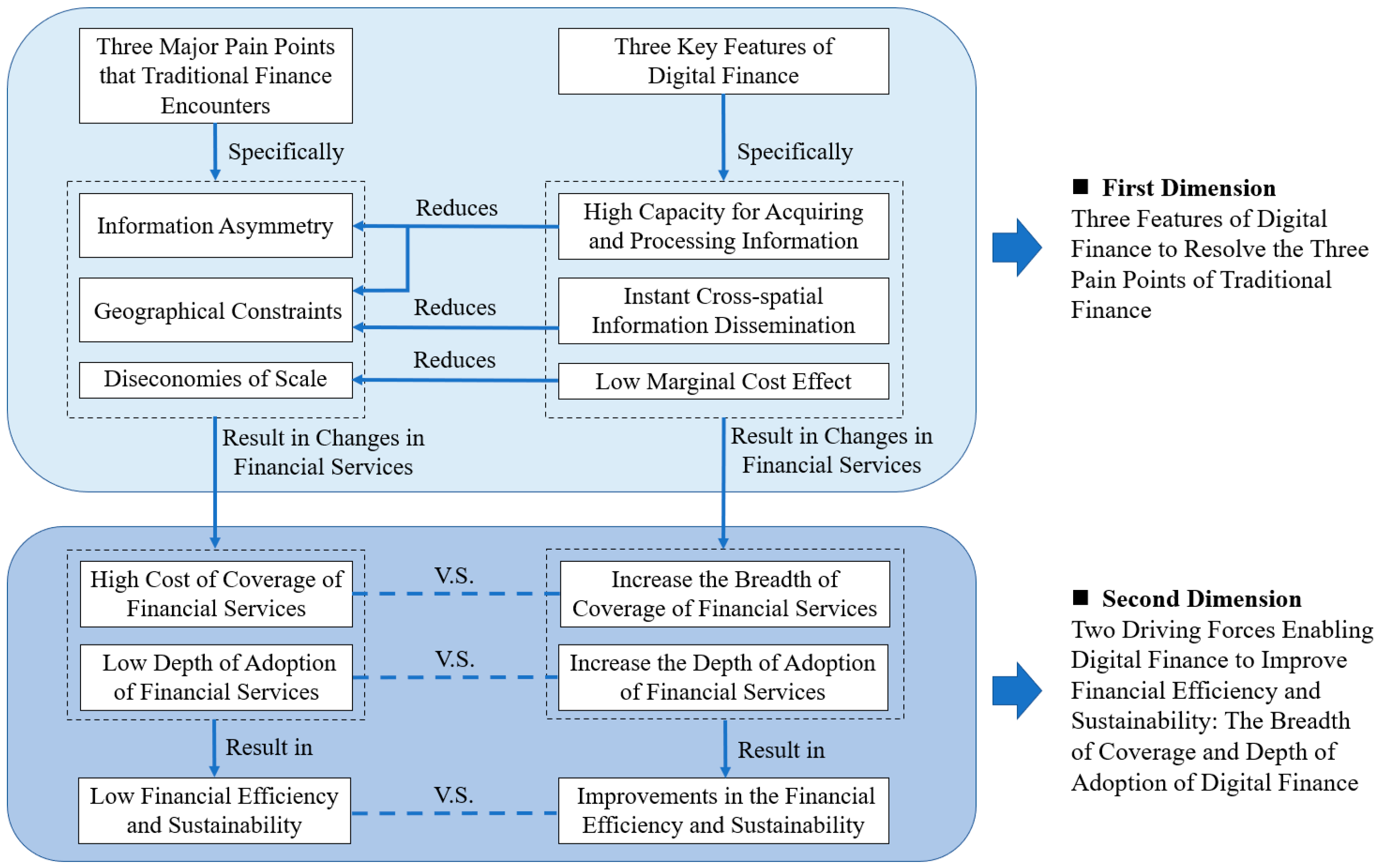
2.3.1. Three Features of Digital Finance to Resolve the Three Pain Points of Traditional Finance

Traditional financial institutions have been reluctant to offer financial services to low-income and remote populations as well as MSMEs [39], because quite often, there are only a limited number of branches in the areas where these customers reside. Hence, they cannot access cash, loans, or other financial services conveniently [40]. Specifically, this is caused by three major pain points in the financial market: firstly, there is information asymmetry. MSMEs and users in low-income and remote areas have difficulties with providing standardized information required for financial risk analysis, such as credit history. Some even do not own bank accounts. This makes it difficult for financial institutions to collect accurate information from them and identify customers who are in need of such services. As a result, they discontinue providing services to these customers to avoid adverse selection and moral hazard problems. Secondly, there are geographical constraints. Traditional financial services are primarily provided by branches of financial institutions, and users need to travel to them on site, which limits the availability of financial services due to information transmission difficulties, transportation costs, and time costs, leaving financial institutions unwilling or unable to provide financial services to remote users. Finally, there are diseconomies of scale. Although demand for financial service remains high, financial institutions cannot achieve economies of scale if the cost of service is too high. With these three pain points, it is challenging for financial institutions to profit from providing financial services to long-tail users; instead, they might have to rely on government policies and targeted subsidies to sustain the service. Under this circumstance, financial efficiency cannot be improved, and the sustainability of financial services are highly likely to be jeopardized.

Nevertheless, digital finance possesses three key features: high capacity for acquiring and processing information, instant cross-spatial information dissemination, and a low marginal cost effect, which can be leveraged to tackle with the three pain points faced by traditional financial institutions in serving long-tail consumers. In particular, as for reducing information asymmetry, digital financial technologies, such as big data, cloud computing, artificial intelligence, and distributed technology, can process massive quantities of data at low cost and low risk [41]. This enables financial institutions to acquire and process information efficiently, and it allows them to build and optimize algorithms and construct big data warehouses [42]. In so doing, financial institutions are capable of systematically embedding massive information into financial services so as to reduce information asymmetry, increase the ability to identify potential financial service users, and pick out qualified users. In this way, financial institutions can improve the efficiency of providing financial services [43]. As for reducing geographical constraints, digital finance has the potential to instantly disseminate information across space [35], thus diminishing the importance of geographical distance, and gradually reducing the geographical boundaries between regions as well as between financial institutions and users [44]. When it comes to limiting diseconomies of scale, the ubiquitous nature of the Internet dictates digital finance a low marginal cost effect, that is, the marginal cost of providing financial services to long-tail users can be significantly reduced with digital technologies [45]. In this case, economies of scale will be as well formed for this group of users.

2.3.2. Two Driving Forces Enabling Digital Finance to Improve Financial Efficiency and Sustainability: The Breadth of Coverage and Depth of Adoption of Digital Finance

In addition, digital finance has contributed to improving financial efficiency by enhancing the breadth of coverage and depth of adoption of digital finance.

With respect to the breadth of digital financial coverage, the number of users covered by financial services determines the size of the demand for financial services. The need for a financial account is a prerequisite for accessing traditional formal financial services, and those without a financial account must physically visit a branch of a financial institution in order to open an account for the first time. As a result, traditional financial institutions will need to increase user coverage by continuously opening new physical branches. Despite the fact that traditional financial institutions can generate income inflow when they reach long-tail customers, the high cost of running branches might lead to economic loss [46]. Consequently, traditional financial systems are more likely to overlook long-tail users. In contrast, by virtue of its ability to immediately disseminate information across space, digital finance can make a significant contribution to reducing geographic barriers of accessing financial services and providing financial services at a lower marginal cost. Therefore, it will facilitate the improvement of financial efficiency and make it possible for financial institutions to provide financial services to long-tail users with benefits outweighing costs and regaining financial sustainability.

When it comes to the depth of digital financial adoption, traditional financial institutions are often the centralized location for almost all financial activities, and most users are required to perform financial activities with physical presence. This is when digital finance could come into use to overcome the geographical constraints of financial services with its capability of instant cross-space dissemination of information, allowing users to access multiple financial services online without visiting a branch. Digital finance can also be leveraged by financial institutions to embed financial services into various daily life scenarios, thanks to its powerful capabilities of information acquisition and processing, as well as low marginal costs borne. It can even facilitate the provision of customized financial services to specific needs. All of these have substantially enhanced the frequency (depth) and efficiency with which consumers utilize various financial services. As an additional benefit, digital finance can also be used to improve the internal business processes of financial institutions, thus improving the overall efficiency of financial services [47].

Thus, overall, the specific mechanisms behind which digital finance improves financial efficiency and sustainability can be summarized as follows: digital finance possesses three key features including a high capacity for acquiring and processing information, instant cross-spatial information dissemination, and a low marginal cost effect → it can be leveraged to resolve the three major pain points that traditional finance encounters when serving long-tail users, i.e., information asymmetry, geographical constraints, and diseconomies of scale → it increases the breadth of coverage and depth of adoption of financial services → this results in improved financial efficiency and financial sustainability. Of course, improvements in the financial efficiency and sustainability of financial institutions at micro level will, in turn, lead to improvements in the financial efficiency and sustainability of the region as a whole.

Accordingly, three theoretical hypotheses are proposed.

Hypothesis 1 (H1).

The development of digital finance contributes to the improvement of financial efficiency positively. The more digital finance is developed, the higher the level of financial efficiency, and the easier it is to achieve sustainable financial development in the region.

Hypothesis 2 (H2).

Among the positive contributors of digital financial development in improving financial efficiency, the breadth of digital financial coverage is one of the core driving forces.

Hypothesis 3 (H3).

Among the positive contributors of digital financial development in improving financial efficiency, the depth of digital financial adoption is one of the core driving forces.

3. Data and Methodology

3.1. Data Description

Table 2. Variable description.

Variables	Description	Measured by
lnSDEA	Financial efficiency level	Regional financial super-efficiency values
IndexAggr	Digital financial development	The Peking University Digital Financial Inclusion Index of China (PKU-DFIIC)
IndexCover	Breadth of digital financial coverage	Sub-index on breadth of coverage of the PKU-DFIIC
IndexUser	Depth of digital financial adoption	Sub-index on depth of adoption of the PKU-DFIIC
AveGDP	Economic development	GDP per capita
FDIRt	Degree of opening-up	Ratio of foreign direct investment to GDP
GovExpenRt	Government expenditure	Ratio of general budget expenditures to GDP
Urbaniz	Level of urbanization	Rate of urbanization
StudNum	Level of education	Number of students enrolled in general higher education institutions
lnAveHousingPrice	Housing conditions	Natural logarithm value of the average housing price
lnPopulation	Population	Natural logarithm value of the resident population
Savings	Household savings	Saving balance of urban and rural residents at year-end
lnRetailSale	Consumption	Natural logarithm value of retail sales for consumer goods
lnLoan	Loan size	Natural logarithm value of loan balance of financial institutions at year-end

Sources: authors’ elaboration.

provides an overview of the main variables examined in this study. For 31 provinces in China from 2011 to 2019, the research employs a dataset covering financial efficiency, digital financial development, and three types of control variables. To begin with, control variables reflecting regional characteristics including economic development, degree of opening-up, government expenditure, urbanization, education, housing conditions, and population. The second type of control variables reflects residential characteristics including household savings and consumption. Finally, the third type of control variables captures the financial characteristics, in this case, loan size. The sources of data are presented as below:

(i)

The Peking University Digital Financial Inclusion Index of China (PKU-DFIIC) [31] is used as a measurement of digital financial development in different regions of China in this paper. The index is released by the Institute of Digital Finance Peking University and derived from the underlying transaction account data from the Chinese digital financial giant Ant Group. It involves three sub-indexes (i.e., first-level dimensions), including breadth of coverage, depth of adoption, and level of digitization. Specifically, the breadth of coverage refers to account coverage, which is measured by three specific indicators such as the number of Alipay accounts per 10,000 people, the proportion of Alipay users who link their Alipay account to bank cards, and the average number of bank cards linked to each Alipay account; the depth of adoption considers the adoption of financial services such as payment, money market fund, loans (personal consumption loan and MSME loan), insurance, investment, and credit investigation, which is measured by 20 specific indicators such as the number of payment transactions per user and the number of purchase transaction of Yu’e Bao per user; the level of digitalization is comprised of four second-level dimensions, which are mobilization, affordability, credit-backed spending, and convenience, including 10 specific indicators such as the proportion of mobile payment transactions, and the average interest rate for MSME loans (cf. Appendix A for details). In addition, the index is calculated by the coefficient of variation method for analytic hierarchy processes. Currently, the index is the predominant choice of data source to study digital finance for Chinese scholars [12,33,34,48].

(ii)

Macroeconomic data at the provincial level, which includes GDP per capita, social financing scale, urbanization rate, population, and total imports and exports, is derived from sources such as China’s regional statistical yearbooks, the WIND database, the Guotaian database (CSMAR), and the Tong Hua Shun-iFind database.

It is worth noting that as mentioned in Section 2.1, this paper adopts the widely agreed definition of financial efficiency from a regional perspective. Financial efficiency is perceived as the degree of financial development of a region or financial system as well as its status of financial resource allocation. Thus, the regional financial efficiency variables in this paper are estimated using the super-efficiency DEA model [23,24,49], which is constructed by input or output indicators such as social fixed asset investment, the number of employees within the financial industry, etc., as detailed in Section 3.2.1 and Section 4.1.

All in all, as panel data are used in the study, a total of 279 observations covering a period of nine years are collected from 31 provinces for each variable.

3.2. Constructing Financial Efficiency Measurement Models

To calculate the financial efficiency level of a region, the study adopts data envelopment analysis (DEA). This method is used for evaluating the effectiveness and resource allocation efficiency of decision-making units (DMUs) with multiple-input and multiple-output. As a non-parametric analysis approach, it does not presume any specific form of production function and instead uses local approximations to determine the relative efficiency of DMUs based on actual observations. As a result of this, a variety of studies using the DEA model have been published, and the model has been widely applied into performance appraisal for a wide range of business scenarios and industrial sectors, becoming one of the most popular techniques for efficiency analysis [50]. Following years of improvement, the method has now diverged into variants such as the CCR model, CCGSS model, BCC model, etc. [51,52,53,54]. One of the key contributions of this paper is to apply the DEA method to financial research. More precisely, the research combines the DEA-BCC model with the super-efficiency DEA model for computing the efficiency of financial resource allocation in each Chinese province, and uses it as a proxy to measure the level of regional financial efficiency.

3.2.1. DEA-BCC Model

In contrast to classical DEA models, the DEA-BCC model relaxes the assumption of constant returns to scale and facilitates the quantification of efficiency gains resulting from scale effects. This makes the DEA-BCC model ideally suited for measuring financial efficiency since the financial sector always has strong scale effects. For this reason, the DEA-BCC model is adopted in this study to estimate the financial efficiency levels of sample regions. Assuming that there are a total number of n independent DMUs in an input–output system denoted as $DM{U}_j$, each of which has the same input variables (a total number of m within each unit) and the same output variables (a total number of s within each unit).

Here, the input variables are denoted by $X_j=(x_{1j},x_{2j},\dots ,x_{mj}{)}^T$, $x_{ij}$ represents the input variable i of the DMU j, and the corresponding weights are denoted by $v={\left(v_1,v_2,\dots ,v_m\right)}^T$; the output variables are denoted by $Y_j=(y_{1j},y_{2j},\dots ,y_{sj}{)}^T$, $y_{rj}$ is the output variable r of the DMU j, and the corresponding weights are denoted by $u={\left(u_1,u_2,\dots ,u_s\right)}^T$. An index for evaluating the efficiency of each DMU is calculated as follows.

$$h_j=\frac{u^T{Y}_j}{v^T{X}_j}=\frac{{{\displaystyle \sum }}_{r=1}^s{u}_r{y}_{rj}}{{{\displaystyle \sum }}_{i=1}^m{v}_i{x}_{ij}}, j=1,2, \dots ,n$$

(1)

Next, an evaluation of the efficiency of DMU $j_0$ is performed using the optimization model constructed under the presumption of variable return to scale, and the Charnes–Cooper transformation is applied so that $t=\frac{1}{{{\displaystyle \sum }}_{i=1}^m{v}_i{x}_{ij}}$, $w=tv$, $\mu =tu$. Thereby, the linear programming model can be expressed as follows.

$$ax{{\displaystyle \sum }}_{r=1}^s{u}_r{y}_{r{j}_0}+\mu$$

(2)

$$s.t. {\displaystyle \sum }_{r=1}^s{\mu }_r{y}_{rj}-{\displaystyle \sum }_{i=1}^m{w}_i{x}_{ij}+\mu \le 0,{\displaystyle \sum }_{i=1}^m{w}_i{x}_{i{j}_0}=1$$

(3)

$$w\ge 0, \mu \ge 0, r=1,2,\dots , s, i=1,2,\dots ,m, j=1,2,\dots ,n$$

(4)

Equation (2) is the objective function of the linear programming model to achieve an optimal solution, while Equations (3) and (4) are used as constraints. Overall, models (1) through (4) are designed to determine the efficiency of DMUs utilizing the optimal solution of the linear programming model. Furthermore, assuming that the optimal solution in linear programming is $h_{j_0}^{*}$, then $DM{U}_{j_0}$ is said to achieve DEA validity if $h_{j_0}^{*}$ = 1, w > 0, and $\mu >0$, whereas all the other cases are invalid. Dual models are constructed to facilitate the economic interpretation and analysis.

$$min\theta$$

(5)

$$s.t. {\displaystyle \sum }_{j=1}^n{\lambda }_j{x}_{ij}\le \theta x_{ij}$$

(6)

$$s.t. {\displaystyle \sum }_{j=1}^n{\lambda }_j{x}_{ij}\ge y_{i{j}_0}, {\displaystyle \sum }_{j=1}^n{\lambda }_j=1$$

(7)

$$\lambda \ge 0, r=1,2,\dots ,s, i=1,2,\dots ,m, j=1,2,\dots ,n$$

(8)

where $\theta$ denotes the efficiency value of each DMU and ${\lambda }_j$ denotes the corresponding weight. Similarly, Equation (5) is the objective function of the linear programming to solve for the optimal solution, whereas Equations (6)–(8) represent the constraints to which the objective is subject. If the optimal solution of the dual model θ equals to 1, then $DM{U}_{j_0}$ is said to be DEA valid, and it is invalid otherwise.

Furthermore, when constructing the DEA-BCC model, based on previous studies [55] and constrained by data availability, this paper selects the social fixed asset investment, variant loan balances of financial institutions, deposit balances of banks, and the number of employees within the financial industry as input indicators, and GDP and value added of financial industry as output indicators. Finally, the study calculates the overall technical efficiency (TE), scale efficiency (SE), and pure technical efficiency (PTE) of financial resource allocation in each region using software DEAP2.1. Specifically, TE is a comprehensive measure of the province’ s ability to allocate and use financial resources. The SE of each province refers to the input–output efficiency influenced by the size of the financial industry; in other words, it is a measure of the gap between the actual size of the financial sector and the optimal size. PTE, on the other hand, refers to the input–output efficiency of the financial industry within each province brought about by technological change; that is, it is a measure of the impact of technological development on financial efficiency.

3.2.2. Super-Efficiency DEA Model

One of the key advantages of the above-mentioned DEA-BCC model is that it is able to measure scale efficiency and pure technical efficiency along with the overall technical efficiency of financial resource allocation, allowing for dismantling and analyzing financial efficiency on multiple dimensions. Yet, there is a weakness that when evaluating the efficiency values of DMUs using the DEA-BCC model, two scenarios of DMUs will emerge. In the first scenario, the efficiency values of DMUs are all within the invalid range; therefore, they can be ranked by efficiency values in descending order. However, for the other scenarios, all the efficiency values are equal to 1. Consequently, it is impossible to further differentiate these efficiency values. In order to overcome this problem, the super-efficiency DEA model [56] is constructed to further distinguish the performance of DMUs on the valid frontier as specified below:

$$\min [\theta -\epsilon >({\displaystyle \sum }_{i=1}^m{s}_i^{-}+{\displaystyle \sum }_{i=1}^s{s}_r^{+}>)]$$

(9)

$$s.t. {\displaystyle \sum }_{\begin{array}{c}j=1\\ j\ne j_0\end{array}}^n{\lambda }_j{x}_{ij}+s_i^{-}=\theta x_{ij}, i=1,2,\dots ,m$$

(10)

$$s.t. {\displaystyle \sum }_{\begin{array}{c}j=1\\ j\ne j_0\end{array}}^n{\lambda }_j{x}_{ij}-s_r^{+}=y_{ij}, r=1,2,\dots ,s$$

(11)

$${\lambda }_j\ge 0, j=1,2,\dots ,n, s_i^{-}\ge 0, s_r^{+}\ge 0$$

(12)

where $s_i^{-}$ and $s_r^{+}$ are slack variables and ε is Archimedean infinitely small (ε is usually set to 0.000001). Similar to Equations (5)–(8), Equation (9) is the objective function to solve for the optimal solution, and Equations (10)–(12) indicate the constraints. If the optimal solution $\theta$= 1, then $DM{U}_{j_0}$ is said to achieve weak DEA validity, and if on top of this, $s_i^{-}$ and $s_r^{+}$ are both zero, then the model is further said to achieve DEA validity. Otherwise, the solutions are invalid.

Note that the super-efficiency DEA model subjects to a constraint $j\ne j_0$, i.e., DMU itself is excluded from its constraint, which is the main feature that distinguishes the super-efficiency DEA model from the DEA-BCC model. As a consequence, the super-efficiency value of the valid DMUs is generally greater than 1, which allows the DMUs on the valid frontier to be further compared. It is for this reason that the financial super-efficiency values derived from the super-efficiency DEA model are used to measure the “financial efficiency level”, that is, the lnSDEA in Table 2. The set of input and output indicators adopted for constructing the DEA-BCC model before are also used in the super-efficiency DEA model here for calculating financial efficiency values.

3.3. Econometric Model

In order to test Hypothesis 1 (H1), this study draws on previous studies [27] to construct an empirical model. Considering the use of panel data spanning over a long period of time requires controlling for time effects as well as for individual effects that are not influenced over time; regression models controlling for the effects of time and individual are first proposed.

$$lnSDE{A}_{ i,t }={\beta }_0+{\beta }_{1}IndexAgg{r}_{i,t}+ {\beta }_2{X}_{,i,t}+{\theta }_t+{\alpha }_i+{\epsilon }_{i,t}$$

(13)

where the dependent variable $lnSDE{A}_{ i,t}$ represents the financial super-efficiency value for province i in year t, as a measure of regional financial efficiency levels (cf. Section 3.2.2 for details). The independent variable $IndexAgg{r}_{i,t}$ represents the value of the Peking University Digital Financial Inclusion Index for province i in year t, as a measure of regional digital financial development. In addition, $X_{,i,t}$ represents other control variables, as displayed in Table 2 above; ${\theta }_t$ represents the control variable for time; ${\alpha }_i$ represents the control variable for region; and ${\epsilon }_{i,t}$ represents the random disturbance term.

Moreover, in order to examine Hypotheses 2 (H2) and 3 (H3), based on Equation (13), the paper uses two indicators of the Digital Financial Inclusion Index, namely the breadth of digital financial coverage and the depth of digital financial adoption, respectively, to investigate the impact of each indicator on financial efficiency. The models are presented as follows:

$$lnSDE{A}_{ i,t }={\beta }_0+{\beta }_{1}IndexCove{r}_{i,t}+ {\beta }_2{X}_{,i,t}+{\theta }_t+{\alpha }_i+{\epsilon }_{i,t}$$

(14)

$$lnSDE{A}_{ i,t }={\beta }_0+{\beta }_{1}IndexUse{r}_{i,t}+ {\beta }_2{X}_{,i,t}+{\theta }_t+{\alpha }_i+{\epsilon }_{i,t}$$

(15)

where $IndexCove{r}_{i,t}$ represents the breadth of digital financial coverage for province i in year t, while $IndexUse{r}_{i,t}$ indicates the depth of digital financial adoption for province i in year t.

4. Empirical Results and Discussions

4.1. Financial Efficiency Analysis by Time and Space

4.1.1. Regional Financial Efficiency Analysis Based on the DEA-BCC Model

Figure 2 demonstrates the trends of the overall technical efficiency (TE), scale efficiency (SE), and pure technical efficiency (PTE) measures of financial resource allocation for 31 provinces in China from 2011 to 2019 (cf. Appendix A for details). It can be seen that PTE remains the highest of the three major financial efficiency indicators, with SE ranking the second and TE ranking the last. Meanwhile, PTE has been increasing steadily over the nine-year period, rising from 0.78 in 2011 to 0.91 in 2019, representing a 16.4% growth rate. SE continues to decline, whereas TE shows a tendency to rise and then drop. This means that from 2011 to 2019, the provincial financial efficiency in China has experienced a period of growth followed by a subsequent phase of decline. While technological advancement has promoted the performance of financial efficiency, the impact of scale effect on financial efficiency has been weakening.

Furthermore, Figure 3 provides a comparison of the three major financial efficiency indicators in 2011 and 2019. First of all, TE values differ considerably between different provinces, with Jiangsu having a mean value equal to 1. This means that the financial resource allocation of Jiangsu consistently reaches the optimal level of DEA efficiency over the past nine years, leading the way for financial efficiency in China. At the same time, Guangdong also has a mean value of TE exceeding 0.9 with several years’ TE values reaching 1 as well. In contrast, the TE values for Tibet, Qinghai, Xinjiang, Hunan, Jilin, and Heilongjiang are relatively low, especially in the latter three provinces, where the average TE values for nine years have not exceeded 0.3. Hence, it is evident that TE is positively related to the geographic location, economic foundation, and market openness of the region. In other words, provinces with location advantages, good economic foundation, and a higher degree of market openness usually have higher TE and vice versa.

However, it is noteworthy that the regional distribution pattern of TE in China over the past nine years has been disrupted, particularly in remote inland regions such as Tibet, Qinghai, and Xinjiang, where the financial efficiency has been significantly improved. This is mainly because in recent years, the Chinese government has actively pushed for its “financial precision poverty alleviation” policy in the central and western regions, emphasizing the need for optimizing the financial ecosystem in poorer areas. At the end of 2019, according to the People’s Bank of China, the loan balances for poverty alleviation amounted to RMB 712.6 billion, serving 19.38 million poor residents in China. Indeed, financial resources are gradually reaching the long-tail users.

Secondly, the average SE value has been declining over the last nine years, implying that the role of scale effect in enhancing financial efficiency is diminishing as the Chinese economy and financial system grow. A possible explanation is the structural change of economic and financial development in China in the aftermath of the 2008 Global Financial Crisis (GFC). Similar to the rest of the world, it also became challenging for China to sustain the economic growth predominantly driven by the expansion of the economic sector before. According to the National Bureau of Statistics, the Chinese GDP growth, which is strongly correlated with SE value, drops sharply from 9.55% to 5.98% over the period of our observations; in addition, the growth rate of social fixed asset investment declines from 20.1% to 5.1%, and the growth rate of value added of financial industry declines from 19.5% to 8.0%. On the other hand, the distribution of SE across various provinces has remained relatively stable, with Jiangsu, Guangdong, Shanghai, Fujian, and Zhejiang on the eastern coasts of China continuing to perform well, while Heilongjiang and Jilin in the northeast, as well as Hunan in central China, have the lowest SE values, with nine-year averages of 0.333, 0.341, and 0.38, respectively. It is because the scale of the regional financial industry is heavily dependent upon factors such as economic condition, population, and geographic location. All of these factors tend to be relatively stable over time, leading to less volatility in the scale of regional financial industry. The conjecture is confirmed in extant literature, indicating that the clustering and expansion of financial industry will exhibit a diminishing positive effect upon regional economic growth and financial efficiency as the Chinese economy continues to grow [57].

Moreover, as is evident from Figure 2, PTE is the best-performing efficiency indicator among the three major ones, and almost all the Chinese provinces have seen significant increases in PTE over the nine-year period. This is mainly because technological advances have contributed remarkably to the improvement of financial efficiency in all regions, with the application of digital technology playing an essential role as a driving force. The advent of Chinese FinTech in 2013 [58] has led to the widespread adoption of technologies such as big data, artificial intelligence, and blockchain in the financial sector, resulting in increased efficiency for financial institutions. It has become common practice among financial institutions to adopt digital financial business models such as big data collections for credit information, big data risk control, and robo-advisory in order to promote the quality of financial services. Mobile banking and securities have also become popular choices for Chinese financial customers.

4.1.2. Regional Financial Efficiency Analysis Based on the Super-Efficiency DEA Model

To further evaluate the financial efficiency of the provinces in China, this study computes the financial super-efficiency values for each province using the super-efficiency DEA model. The results are illustrated in

Table 3. Financial super-efficiency values (SDEA) by province in China, from 2011 to 2019.

	2011	2012	2013	2014	2015	2016	2017	2018	2019	Mean
Jiangsu	1.044	1.273	1.271	1.314	1.202	1.188	1.128	1.193	1.111	1.192
Guangdong	1.068	1.003	1.03	0.931	1.068	1.008	0.997	0.962	1.16	1.025
Tianjin	1.09	1.199	1.188	1.126	0.873	0.71	0.606	0.609	0.498	0.878
Shanghai	0.912	0.811	0.735	0.745	0.815	0.85	0.928	0.914	0.92	0.848
Beijing	0.841	0.842	0.758	0.744	0.724	0.736	0.716	0.833	0.828	0.780
Zhejiang	1.022	0.876	0.696	0.587	0.528	0.511	0.527	0.532	0.649	0.659
Chongqing	0.652	0.607	0.591	0.613	0.702	0.744	0.749	0.728	0.523	0.657
Fujian	0.681	0.603	0.609	0.593	0.622	0.604	0.587	0.68	0.59	0.619
Hubei	0.465	0.474	0.506	0.519	0.629	0.7	0.729	0.766	0.712	0.611
Yunnan	0.493	0.455	0.505	0.547	0.652	0.668	0.678	0.612	0.61	0.580
Shandong	0.612	0.634	0.613	0.591	0.554	0.577	0.558	0.539	0.541	0.580
Sichuan	0.446	0.523	0.544	0.525	0.563	0.569	0.601	0.549	0.493	0.535
Qinghai	0.319	0.298	0.44	0.491	0.648	0.655	0.72	0.633	0.469	0.519
Guangxi	0.43	0.419	0.474	0.488	0.507	0.504	0.516	0.475	0.387	0.467
Henan	0.404	0.402	0.408	0.438	0.54	0.477	0.503	0.474	0.489	0.459
Ningxia	0.489	0.441	0.441	0.423	0.45	0.446	0.467	0.433	0.396	0.443
Tibet	0.345	0.303	0.283	0.369	0.501	0.622	0.49	0.613	0.459	0.443
Guizhou	0.426	0.392	0.369	0.369	0.464	0.484	0.511	0.518	0.377	0.434
Inner Mongolia	0.454	0.392	0.397	0.417	0.474	0.534	0.557	0.418	0.219	0.429
Jiangxi	0.349	0.327	0.339	0.399	0.472	0.514	0.496	0.453	0.398	0.416
Anhui	0.342	0.328	0.394	0.403	0.429	0.412	0.418	0.452	0.522	0.411
Hainan	0.509	0.369	0.44	0.384	0.392	0.419	0.387	0.327	0.394	0.402
Liaoning	0.372	0.396	0.411	0.422	0.475	0.429	0.413	0.344	0.306	0.396
Xinjiang	0.374	0.363	0.373	0.388	0.413	0.385	0.378	0.358	0.467	0.389
Shanxi	0.374	0.359	0.382	0.386	0.448	0.428	0.423	0.274	0.202	0.364
Shaanxi	0.332	0.332	0.36	0.399	0.397	0.368	0.345	0.347	0.318	0.355
Hebei	0.347	0.345	0.343	0.342	0.327	0.341	0.353	0.327	0.348	0.341
Gansu	0.215	0.201	0.267	0.316	0.392	0.421	0.39	0.403	0.466	0.341
Hunan	0.271	0.256	0.272	0.294	0.304	0.318	0.358	0.326	0.289	0.299
Jilin	0.209	0.19	0.255	0.265	0.316	0.346	0.347	0.289	0.247	0.274
Heilongjiang	0.274	0.271	0.282	0.285	0.3	0.267	0.245	0.23	0.219	0.264

Note: the above provinces are ranked according to the average SDEA values from 2011 to 2019. Sources: authors’ elaboration.

below.

As can be seen, for provinces whose SDEA fall within the invalid range, the super-efficiency values are largely the same as those calculated by the DEA-BCC model. However, for provinces with valid SDEA values, the super-efficiency values often exceed 1 and vary, indicating that this model is able to capture the nuances among “leading players” in terms of financial efficiency. In particular, Jiangsu, Guangdong, Tianjin, Shanghai, and Beijing are among the highest-ranking regions in China in terms of SDEA, with mean values of 1.192, 1.025, 0.878, 0.848, and 0.780, respectively. While Heilongjiang, Jilin, and Hunan remain the provinces with the lowest financial efficiency in the country, having SDEA values of only 0.264, 0.274, and 0.299 separately. All in all, it is obvious that most provinces with higher financial efficiency are economically more developed and their advantages tend to be prolonged. This is most likely because their strengths in economic foundation and industrial structure have effectively contributed to the long-term development of their financial sectors. The findings are also manifested in existing studies that indicate that the efficiency of financial resource allocation tends to be higher in economically more developed regions such as the eastern area, and it tends to be lower in the middle and western regions [55].

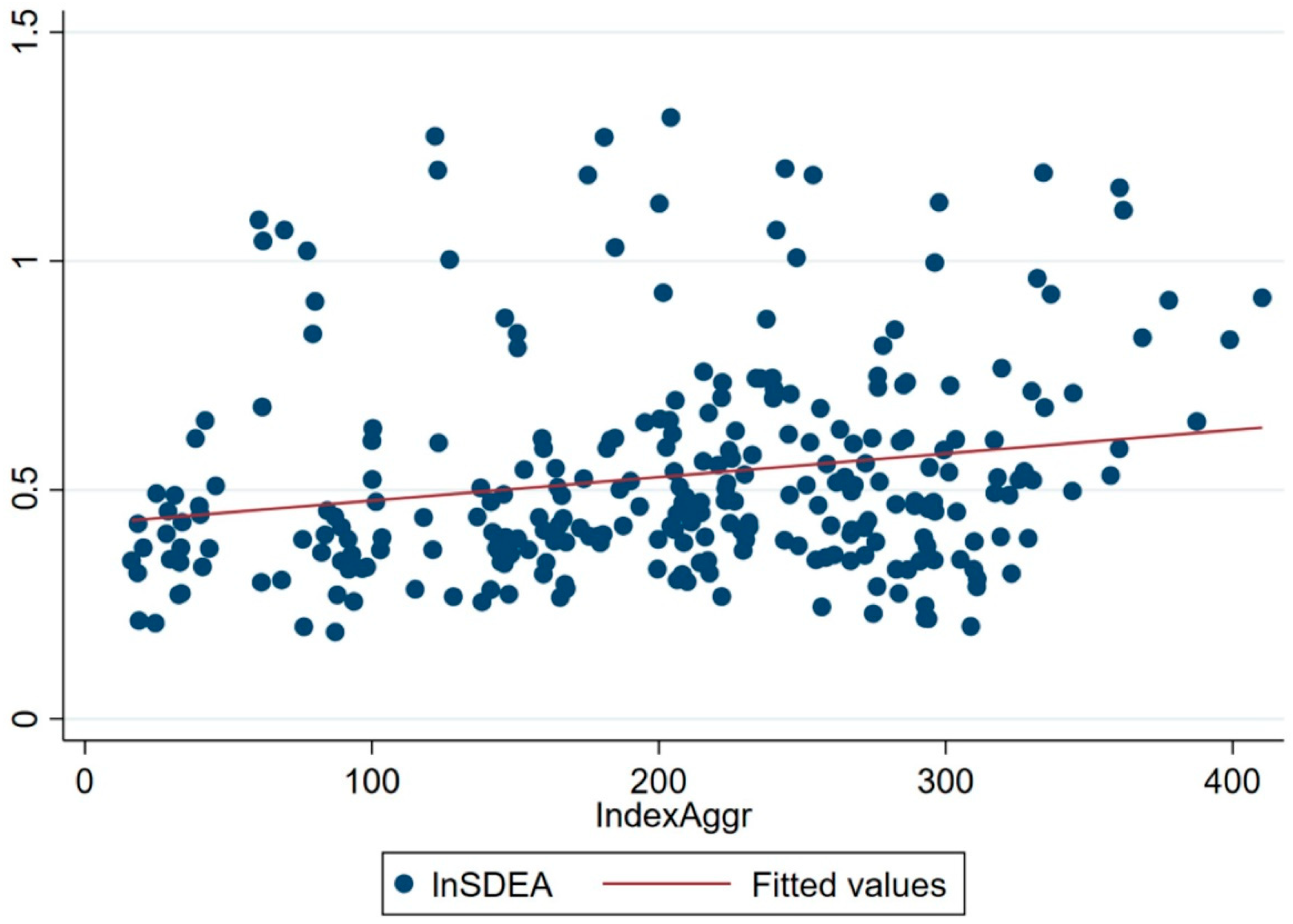
4.2. Impact of Digital Financial Development on Financial Efficiency

Table 4. Descriptive statistics.

	Mean	Standard Deviation	Median	Minimum	Maximum
lnSDEA	0.53	0.23	0.47	0.19	1.31
IndexAggr	202.35	91.65	212.36	16.22	410.28
IndexCover	182.25	90.47	189.28	1.96	384.66
IndexUser	197.02	91.46	189.78	6.76	439.91
AveGDP	54,017.93	26,223.36	46,674.00	16,413.00	164,000.00
FDIRt	0.02	0.02	0.02	0.01	0.08
GovExpenRt	0.28	0.21	0.23	0.11	1.38
Urbaniz	56.66	13.14	55.12	22.71	89.60
StudNum	84.17	52.78	73.25	3.24	231.97
lnAveHousingPrice	8.79	0.47	8.65	8.09	10.49
lnPopulation	8.13	0.84	8.25	5.74	9.43
Savings	17,190.30	14,184.78	13,399.44	178.40	77,995.87
lnRetailSale	8.73	1.05	8.88	5.47	10.67
lnLoan	9.98	0.94	10.02	6.01	12.03

Sources: authors’ elaboration.

summarizes the descriptive statistics derived from our data for 31 Chinese provinces from 2011 to 2019. As can be seen, the standard deviations of certain variables such as financial efficiency, digital financial development, economic development, degree of opening-up, and government expenditure are all high across provinces. However, it is evident that regional disparities persist. For example, the mean value for financial efficiency is 0.53, with a standard deviation of 0.23. Meanwhile, the mean value for the digital financial inclusion development index is 220.35, with a standard deviation of 91.6. In addition, although the distribution for the variables across Chinese provinces suggest a certain degree of skewness, the differences between the mean and median values are not significant, indicating that the distribution of variables is fairly close to normal distribution.

On the basis of the descriptive statistics, this study first conducts the preliminary analysis on the correlation between digital financial development and the financial efficiency in various provinces. As shown in Figure 4, it is apparent that digital finance and financial efficiency exhibit a relatively strong positive correlation; therefore, it is assumed that digital finance is likely to improve financial efficiency. This preliminary result will be further tested as follows.

To test Hypothesis 1 (H1), this paper first tests the stationarity of the variables using the Augmented Dickey–Fuller unit root test (ADF unit root test), and all the variables are stationary, I(0) (cf. Appendix A for details). Then, Pesaran’s test, Friedman’s test, and Frees’ test are performed for each variable in accordance with Equation (13), the results of which indicate the existence of cross-sectional correlation problems. Afterwards, dummy variables are incorporated into the model, and the least squared dummy variable model (LSDV model, which is a branch of the fixed effects model) is used to control the cross-sectional correlation problem of the error terms; this is followed by a Hausman test. All the results are in favor of the random effects model. Having confirmed that the model is free of autocorrelation and heteroskedasticity problems, this paper finally constructs a random effects model controlling for cross-sectional correlation problems for the hypothesis test.

In addition, control variables are incorporated step by step into the random effects model in order to observe the specific influence of these control variables on the statistical significance of the results. First, the model controls only for variables reflecting regional characteristics, as shown in column 1 of

Table 5. Random effects regression results of digital financial development on financial efficiency.

	(1)	(2)	(3)
	RE	RE	RE
IndexAggr	0.002	0.003 **	0.003 **
	(1.34)	(1.89)	(1.91)
AveGDP	0.000 *	0.000 *	0.000
	(1.81)	(1.98)	(1.65)
FDIRt	−0.111	−0.596	0.496
	(−0.04)	(−0.23)	(0.20)
GovExpenRt	0.250 *	0.430 ***	0.246 **
	(1.92)	(3.20)	(2.35)
Urbaniz	0.003	0.008 ***	−0.001
	(1.12)	(2.85)	(−0.14)
StudNum	0.001	0.002	0.002
	(0.65)	(1.35)	(1.51)
lnAveHousingPrice	−0.013	−0.027	−0.110
	(−0.11)	(−0.25)	(−0.98)
lnPopulation	−0.057	0.004	0.000 ***
	(−1.16)	(0.04)	(3.78)
Savings		0.000 ***	−0.107
		(3.96)	(−1.21)
lnRetailSale		−0.054	0.346 ***
		(−0.59)	(3.72)
lnLoan			0.250 *
			(1.81)
Observations	279	279	279
Controlling for time effects	Y	Y	Y
Controlling for individual effects	N	N	N
Adj. R2	0.591	0.630	0.683
F value	73.60	144.94	164.89

Note: t-statistics are presented in parentheses, *, **, and *** denote statistical significance at the 10%, 5%, and 1% levels, respectively. Sources: authors’ elaboration.

. As can be seen in column 2 of the table, variables related to both regional and residential characteristics are controlled. Afterwards, the model controls for all three types of variables, i.e., variables representing regional, residential, and financial characteristics, as shown in column 3 of Table 5. The empirical results reveal that as a whole, the coefficients of digital financial development are positive in each model, suggesting that digital financial development does indeed have a positive impact on regional financial efficiency. As more control variables are incorporated, the coefficient of digital finance starts to shift from statistically insignificant to significant at the 5% level, with the coefficient stabilizing at 0.003. Hence, this means that the research Hypothesis 1 (H1) has been verified, and the development of digital finance does significantly contribute to the improvement of financial efficiency, thus enhancing financial sustainability.

Furthermore, the coefficients for government expenditure are significantly positive in all the models, suggesting that government expenditures can notably promote the financial efficiency of a region in China. It is most likely because higher government expenditure can reflect the local government’s ability to create a more conducive business environment or to introduce policies that are more favorable to local financial industry. As a result, greater financial efficiency will be achieved. In addition, economic development, urbanization, population, household savings, as well as consumption may also have positive effects on regional financial efficiency, which to some degree confirms the findings discussed in Section 4.1; i.e., the greater the economic development, the higher the level of local financial efficiency.

4.3. Impact of Breadth of Coverage and Depth of Adoption of Digital Finance on Financial Efficiency

In response to Hypotheses 2 (H2) and 3 (H3), this research proceeds to further investigate the impact of the breadth of coverage and depth of adoption of digital finance on financial efficiency in accordance with Equations (14) and (15), respectively. The analytical procedure is the same as that in Section 4.2, yet, by contrast with the baseline model, the test results here support the selection of LSDV model for further analysis. In

Table 6. LSDV results of the breadth of coverage and depth of adoption of digital finance on financial efficiency.

	(1)	(2)
	LSDV	LSDV
IndexCover	0.005 ***
	(3.13)
IndexUser		0.001 ***
		(2.55)
AveGDP	0.000	0.001 ***
	(0.24)	(3.25)
FDIRt	1.136	0.103
	(0.49)	(0.12)
GovExpenRt	0.080	0.178
	(0.16)	(1.60)
Urbaniz	−0.003	−0.001
	(−0.36)	(−0.27)
StudNum	0.000	0.002 ***
	(0.16)	(3.37)
lnAveHousingPrice	−0.096	−0.092 *
	(−0.56)	(−1.79)
lnPopulation	1.557 **	0.292 ***
	(2.10)	(3.77)
Savings	0.000	0.000 ***
	(0.99)	(5.57)
lnRetailSale	0.185 ***	−0.083
	(2.79)	(−1.51)
lnLoan	0.261 ***	0.351 ***
	(3.97)	(6.65)
Observations	279	279
Controlling for time effects	Y	Y
Adj. R2	0.915	0.680
F value	174.30	45.80

Note: t-statistics are presented in parentheses; *, **, and *** denote statistical significance at the 10%, 5%, and 1% levels, respectively. Sources: authors’ elaboration.

, the regression results for the breadth of digital financial coverage are reported in column 1, while those for the depth of digital financial adoption are reported in column 2.

Clearly, it is found that both the breadth of coverage and depth of adoption of digital finance have a significant positive impact on financial efficiency at the 1% significance level, with a relatively higher coefficient of 0.005 for breadth of coverage and lower coefficient of 0.0001 for depth of adoption. This means that both Hypotheses 2 (H2) and 3 (H3) are supported, i.e., the positive contribution of digital financial development to financial efficiency is pronounced for both variables. Moreover, the positive driving effect of the breadth of coverage is stronger than that of the depth of adoption. The reason for this is that digital finance, with its powerful data acquisition and processing capabilities, instantaneous spatial dissemination of information, and low marginal costs, can directly contribute to improving financial efficiency by serving a large number of users who were previously difficult to serve by traditional financial services, significantly increasing the coverage of financial services. On the other hand, the penetration of financial services into a wider range of businesses and daily life scenarios reflected by the depth of digital financial adoption is considerably more difficult and complex.

4.4. Robustness Checks

Econometrically, the estimation of Equations (13)–(15) may generate endogeneity issues: regions with higher financial efficiency may themselves be more financially literate and accept digital finance more readily. This may ultimately lead to more successful digital financial development. Furthermore, the financial efficiency level and digital financial development may be influenced simultaneously by a range of unobservable factors, resulting in biased estimates of the regression coefficients. Hence, the study uses both instrumental variables and an alternative estimation model to test the robustness of the baseline results.

4.4.1. Instrumental Variable Regression

As an alternative for the digital financial development of a region, this paper utilizes mobile phone ownership per capita in Chinese provinces as an instrumental variable to run the regression using the same baseline model.

First, in terms of exogeneity, mobile phone ownership per capita reflects the IT development in the region itself, since it is primarily dependent on factors such as the degree of local IT development and does not significantly correlate with the intensity of local financial activities; thus, it is clearly exogenous to local financial efficiency. Second, in terms of correlation, the F-value of digital financial development and per capita mobile phone ownership is 2399.09, which passes the correlation test at a value greater than 10, indicating that there is a strong correlation between regional digital financial development and mobile phone ownership per capita, free of the weak instrumental variables problem. Next, for the endogeneity test, the results of the Hausman test on an alternative instrumental variable indicate that there is indeed an endogeneity issue in the model; hence, the use of instrumental variable regression is justified.

In

Table 7. Robustness check for the baseline regression: instrumental variable regression.

	(1)	(2)	(3)
	RE	RE	RE
PerMobile	0.584 ***	0.584 ***	0.452 ***
	(5.12)	(4.14)	(3.46)
AveGDP	0.000 **	0.000 **	0.000
	(2.63)	(2.18)	(1.26)
FDIRt	−1.914	−2.220	−1.573
	(−0.82)	(−0.95)	(−0.67)
GovExpenRt	0.279 *	0.342 **	0.172
	(1.94)	(2.10)	(0.93)
Urbaniz	0.009 ***	0.010 ***	0.001
	(2.78)	(2.84)	(0.14)
StudNum	−0.000	0.000	0.002
	(−0.16)	(0.10)	(1.24)
lnAveHousingPrice	0.133 *	0.145 *	0.042
	(1.70)	(1.72)	(0.38)
lnPopulation	0.070	0.146	0.359 **
	(1.44)	(1.05)	(2.08)
Savings		0.000 ***	0.000
		(3.20)	(0.39)
lnRetailSale		0.073	−0.017
		(0.72)	(−0.18)
lnLoan			0.397 ***
			(3.56)
Observations	279	279	279
Controlling for time effects	Y	Y	Y
Controlling for individual effects	N	N	N
Adj.R2	0.636	0.668	0.658
F value	158.62	204.4	131.88

Note: t-statistics are presented in parentheses; *, **, and *** denote statistical significance at the 10%, 5%, and 1% levels, respectively. Sources: authors’ elaboration.

, the results of regression on instrumental variables based on the baseline model (i.e., a random effects model controlling for cross-sectional correlation problems) are reported, and the control variables are incorporated incrementally to see whether and how they change the statistical significance of the model. More precisely, column 1 shows the results of the regression that control only for the variables accounting for regional characteristics, column 2 presents the results of the regression that control for both variables reflecting the regional characteristics and resident characteristics, whilst column 3 displays the results of the regression with all these three types of variables controlled. Accordingly, the results of the instrumental variable regression are similar to those of the baseline model, indicating that the empirical results of the baseline model are robust.

4.4.2. Alternative Estimation Model

As a further step for robustness checks, this research uses the second-order least-squared estimation of random effects (EC2SLS) and two-stage least squared estimation with two-way fixed effects (FE2SLS), respectively, and compares them with the results of the fixed effects model. The findings are presented in

Table 8. Robustness check for the baseline regression: alternative estimation model.

	(1)	(2)	(3)
	EC2SLS	FE2SLS	FE
IndexAggr	0.002 ***	0.036 **	0.003 **
	(8.85)	(2.36)	(2.54)
AveGDP	0.000 ***	0.000	0.000 ***
	(2.85)	(1.34)	(2.96)
FDIRt	0.260	−1.976	0.496
	(0.30)	(−1.09)	(0.62)
GovExpenRt	0.159	1.112 **	0.246 **
	(1.31)	(2.44)	(2.13)
Urbaniz	−0.004	0.019 *	−0.001
	(−1.47)	(1.71)	(−0.23)
StudNum	0.002 ***	0.006 ***	0.002 ***
	(3.89)	(3.25)	(3.56)
lnAveHousingPrice	0.019	−1.101 **	−0.110 **
	(0.42)	(-2.34)	(−1.97)
lnPopulation	0.313 ***	0.433	0.250 ***
	(3.65)	(1.27)	(3.10)
Savings	−0.000	0.000 **	0.000 ***
	(−0.60)	(2.21)	(5.61)
lnRetailSale	−0.018	0.812 **	0.107 *
	(−0.31)	(2.40)	(1.84)
lnLoan	0.379 ***	0.338 ***	0.346 ***
	(6.65)	(3.06)	(6.54)
Observations	279	279	279
Controlling for time effects	Y	Y	Y
Controlling for individual effects	N	Y	Y
Adj.R2	0.617	0.106	0.680
F value	-	-	45.80
Wald Chi2	418.01	1090.53	-

Note: t-statistics are presented in parentheses; *, **, and *** denote statistical significance at the 10%, 5%, and 1% levels, respectively. Sources: authors’ elaboration.

. It is found that the results from all three models are consistent with those of the baseline model, and the explanatory variable digital financial development is significant at the 1%, 5%, and 5% levels, respectively. This further confirms the robustness of the baseline results and the fact that the development of digital finance has an important impact on financial efficiency.

5. Conclusions

The purpose of this paper is to study whether digital finance could contribute to the promotion of financial sustainability by taking the financial efficiency as an entry point. The research first summarizes the theoretical mechanism for digital finance to improve financial efficiency and sustainability, and it puts forward three major hypotheses. It is found that digital finance possesses three features, i.e., high capacity for acquiring and processing information, instant cross-spatial information dissemination, and a low marginal cost effect. All of these three features can be leveraged to resolve the three major pain points, i.e., information asymmetry, geographical constraints, and diseconomies of scale, to serving long-tail users faced by traditional financial institutions, thus enhancing financial sustainability and efficiency.

Second, a DEA-BCC model and a super-efficiency DEA model are constructed to estimate a series of financial efficiency values of 31 provinces in China, encompassing the overall technical efficiency, scale efficiency, and pure technical efficiency of financial resource allocation, as well as super-efficiency values. The findings show that, as for the temporal trend, the financial efficiency of Chinese provinces has undergone significant changes over time, with a progressively increasing pure technical efficiency and declining scale efficiency. This means that technological advances have contributed greatly to the improvement of financial efficiency, while the role of scale effect in enhancing financial efficiency is diminishing. As for the geographical distribution, Jiangsu, Guangdong, Tianjin, Shanghai, and Beijing are among the top regions in China for financial efficiency, while Heilongjiang, Jilin, and Hunan have the lowest financial efficiency. It is also noteworthy that the financial performances of remote inland regions such as Tibet, Qinghai, and Xinjiang have improved significantly over the past nine years, which is driven primarily by the improvement in technical efficiency, that is, the more obvious role of technology in promoting financial performances in remote and poor regions.

Furthermore, using data from 31 provinces in China from 2011 to 2019, this study employs a random effects model controlling for cross-sectional correlation problems and an LSDV model to investigate whether digital financial development can contribute to the promotion of financial efficiency, and if so, whether this can be achieved by improving its breadth of coverage and depth of adoption. The results confirm all three theoretical hypotheses. Specifically, the development of digital finance can significantly contribute to the improvement of regional financial efficiency. Government expenditure, economic development, urbanization level, population, household savings, and consumption can also influence regional financial efficiency. In addition, both the breadth of coverage and the depth of adoption of digital finance have a significant positive effect on financial efficiency at the 1% significance level, with a greater coefficient of breadth of coverage than that of the depth of adoption. This may imply that both the breadth and depth of digital finance are essential for the positive impact of digital finance to take effect on financial efficiency, and between the two, the positive impact of the breadth of coverage is more evident.

Our findings provide valuable insights for policymakers and financial institutions to achieve financial sustainability goals. It should be recognized that first of all, technological advancement is indeed essential to financial efficiency. The adoption and advancement of digital technologies, such as big data, cloud computing, and blockchain, are important for the financial industry, and they must be continuously promoted. Additionally, one should strengthen the construction of digital infrastructure and leverage the ever-upgrading digital technologies in order to boost the financial sector. Second, given that digital finance may enhance financial efficiency, policymakers could implement targeted policies, tax breaks, government industrial funds, and other means to support the growth of digital finance. Financial institutions should, on the other hand, intensify their investments in digital finance, while recruiting and cultivating comprehensive digital financial talents. Moreover, efforts should be put forward to enhance the coverage of digital finance and accelerate its penetration into various application scenarios to strengthen its depth of adoption. These efforts can more effectively contribute to the improvement of local financial efficiency. To summarize, we must strengthen the underlying technologies while improving the breadth of coverage and depth of adoption of digital finance. In so doing, the impact of digital finance could potentially be maximized on promoting financial efficiency. Thus, financial institutions will be able to provide more inclusive and economic financial services as well as promote the sustainable development of the financial industry and society as a whole.

The limitations of this paper are twofold. Constrained by the availability of data, the study is only able to employ a set of panel data at the provincial level for China. In the future, the adoption of municipal level or even county-level data may enhance the thoroughness of arguments and robustness of the study. In addition, this study is focused primarily on regional aspects, but it has neither dug into the analysis at the micro dimension, i.e., the efficiency of financial institutions, nor into the interactions between the regional financial efficiency and institutions within the region. This can be further explored.

References

1. Bruhn, M.; Hommes, M.; Khanna, M.; Singh, S.; Sorokina, A.; Wimpey, J. MSME Finance Gap: Assessment of the Shortfalls and Opportunities in Financing Micro, Small, and Medium Enterprises in Emerging Markets; World Bank: Washington, DC, USA, 2017. [Google Scholar]
2. United Nations ESCAP. Transforming Our World: The 2030 Agenda for Sustainable Development; United Nations: New York, NY, USA, 2015. [Google Scholar]
3. Allen, H. Village Savings, Loans Associations-Sustainable and Cost-Effective Rural Finance. Small Enterp. Dev. 2006, 17, 61. [Google Scholar] [CrossRef]
4. Yip, A.W.H.; Bocken, N.M.P. Sustainable Business Model Archetypes for the Banking Industry. J. Clean Prod. 2018, 174, 150–169. [Google Scholar] [CrossRef]
5. Weston, P.; Nnadi, M. Evaluation of Strategic and Financial Variables of Corporate Sustainability and ESG Policies on Corporate Finance Performance. J. Sustain. Financ. Invest. 2021, 11, 1–17. [Google Scholar] [CrossRef]
6. Puschmann, T.; Leifer, L. Sustainable Digital Finance: The Role of FinTech, InsurTech & Blockchain for Shaping the World for the Better; University of Zurich: Zurich, Switzerland; Stanford University: Standford, CA, USA, 2020. [Google Scholar]
7. Gomber, P.; Koch, J.A.; Siering, M. Digital Finance and FinTech: Current research and future research directions. J. Bus. Econ. 2017, 87, 537–580. [Google Scholar] [CrossRef]
8. Global Partnership for Financial Inclusion. G20 High Level Principles for Digital Financial Inclusion; Group of 20: Hangzhou, China, 2016. [Google Scholar]
9. Demirgüç-Kunt, A.; Leora, K.; Dorothe, S.; Saniya, A.; Jake, H. The Global Findex Database 2017: Measuring Financial Inclusion and the Fintech Revolution; World Bank: Washington, DC, USA, 2018. [Google Scholar]
10. United Nations. Inter-Agency Task Force on Financing for Development, Financing for Sustainable Development Report 2020; United Nations: New York, NY, USA, 2020. [Google Scholar]
11. Bauer, J.M. The Internet and Income Inequality: Socio-economic Challenges in a Hyperconnected Society. Telecommun. Policy 2018, 42, 333–343. [Google Scholar] [CrossRef]
12. Yi, X.J.; Zhou, L. Does the Development of Digital Inclusive Finance Significantly Affect Resident Consumption—Micro Evidence from Chinese Households. J. Financ. Res. 2018, 11, 47–67. [Google Scholar]
13. Zhang, X.; Yang, T.; Wang, C. Digital Financial Development and Consumer Growth: Theory and Practice in China. J. Manag. World 2020, 36, 48–63. [Google Scholar]
14. Dillip, K.D. Migration of Financial Resources to Developing Countries; Macmillan Publ. Co.: Hampshire, UK, 1986. [Google Scholar]
15. Hsieh, C.T.; Klenow, P.J. Misallocation and Manufacturing TFP in China and India. Q. J. Econ. 2009, 124, 1403–1448. [Google Scholar] [CrossRef] [Green Version]
16. Brandt, L.; Tombe, T.; Zhu, X. Factor Market Distortions across Time, Space and Sectors in China. Rev. Econ. Dyn. 2013, 16, 39–58. [Google Scholar] [CrossRef] [Green Version]
17. Ozili, P.K. Impact of Digital Finance on Financial Inclusion and Stability. Borsa Istanb. Rev. 2018, 18, 329–340. [Google Scholar] [CrossRef]
18. Dupas, P.; Karlan, D.; Robinson, J. Banking the Unbanked? Evidence from Three Countries. Am. Econ. J.-Appl. Econ. 2018, 10, 257–297. [Google Scholar] [CrossRef] [Green Version]
19. Widarwati, E.; Solihin, A.; Nurmalasari, N. Digital Finance for Improving Financial Inclusion Indonesians’ Banking. J. Ilmu. Econ. 2022, 11, 17–30. [Google Scholar] [CrossRef]
20. Bettinger, A. Fintech: A series of 40 Time shared models used at Manufacturers Hanover Trust Company. Interfaces 1972, 2, 62–63. [Google Scholar]
21. Arner, D.W.; Janos, B.; Ross, P.B. The evolution of Fintech: A new post-crisis paradigm. Georget. J. Int. Law. 2015, 47, 1271. [Google Scholar] [CrossRef] [Green Version]
22. Huang, Y.P.; Huang, Z. China’s Digital Financial Development: Now and the Future. Q. Econ. 2018, 17, 1489–1502. [Google Scholar]
23. Wurgler, J. Financial Markets and the Allocation of Capital. J. Financ. Econ. 2000, 58, 187–214. [Google Scholar] [CrossRef] [Green Version]
24. Zhou, G.F.; Hu, H.M. Research on Financial Efficiency Evaluation Index System. Financ. Theory Pract. 2007, 8, 15–18. [Google Scholar]
25. Brundtland, G. Report of the World Commission on Environment and Development: Our Common Future; United Nations: New York, NY, USA, 1987. [Google Scholar]
26. Zhang, J.T. Research on The Sustainability of Financial Inclusion Business Based on the Internet Perspective. J. Financ. Econ. 2017, 2, 71–74. [Google Scholar]
27. Gong, G.; Jiang, Z.L.; Xu, D.S. The Dynamic Evolution of Shadow Banking and Resource Allocation Efficiency of Non-Financial Firms. Q. Econ. 2021, 21, 2105–2126. [Google Scholar]
28. Shahbaz, M.; Nasir, M.A.; Lahiani, A. Role of Financial Development in Economic Growth in the Light of Asymmetric Effects and Financial Efficiency. Int. J. Financ. Econ. 2022, 27, 361–383. [Google Scholar] [CrossRef]
29. Lu, X.D. Is Financial Resource Mismatch Hindering China’s Economic Growth? J. Financ. Res. 2008, 4, 55–68. [Google Scholar]
30. Deloitte. A Tale of 44 Cities—Connecting Global Fintech: Interim Hub Review; Deloitte: New York, NY, USA, 2017. [Google Scholar]
31. Guo, F.; Wang, J.Y.; Wang, F.; Kong, T.; Zhang, X.; Cheng, Z.Y. Measuring the Development of Digital Inclusive Finance in China: Indexing and Spatial Characteristics. Q. Econ. 2020, 19, 1401–1418. [Google Scholar]
32. Zhan, M.H.; Zhang, C.R.; Shen, J. Internet Finance Development and the Bank Credit Channel Transmission of Monetary Policy. Econ. Res. J. 2018, 53, 63–76. [Google Scholar]
33. Wang, X.H.; Zhao, Y.X. Is There a Matthew Effect in Digital Financial Development? Empirical Comparison of Poor and Non-Poor Households. J. Financ. Res. 2020, 7, 114–133. [Google Scholar]
34. Xie, X.L.; Shen, Y.; Zhang, H.X.; Guo, F. Can Digital Finance Promote Entrepreneurship? Evidence from China. Q. Econ. 2018, 17, 1557–1580. [Google Scholar]
35. Li, W.Q. Research on Internet Finance to Crack the Financing Dilemma of Small and Medium-sized Enterprises. Acad. J. Zhon. 2014, 8, 51–54. [Google Scholar]
36. Jiao, J.P. The Development of Inclusive Finance Should Adhere to the Principle of Sustainable Business. Tsinghua Financ. Rev. 2016, 12. [Google Scholar] [CrossRef]
37. Le, T.H.; Chuc, A.T.; Taghizadeh-Hesary, F. Financial Inclusion and Its Impact on Financial Efficiency and Sustainability: Empirical Evidence from Asia. Borsa Istanb. Rev. 2019, 19, 310–322. [Google Scholar] [CrossRef]
38. Bachelet, M.J.; Becchetti, L.; Manfredonia, S. The Green Bonds Premium Puzzle: The Role of Issuer Characteristics and Third-Party Verification. Sustainability 2019, 11, 1098. [Google Scholar] [CrossRef] [Green Version]
39. Morduch, J.; Armendariz, B. The Economics of Microfinance; MIT Press: Cambridge, MA, USA, 2005. [Google Scholar]
40. Wen, T.; Zhu, J.; Wang, X.H. Elite Capture Mechanism of Agricultural Loans In China: A Stratified Comparison of Poor and Non-Poor Counties. J. Econ. Res. 2016, 51, 111–125. [Google Scholar]
41. Gomber, P.; Kauffman, R.J.; Parker, C. On the Fintech Revolution: Interpreting the Forces of Innovation, Disruption, and Transformation in Financial Services. J. Manag. Inform. Syst. 2018, 35, 220–265. [Google Scholar] [CrossRef]
42. Xie, P.; Zou, C.W. Model Study on Internet Finance. J. Financ. Res. 2012, 12, 11–22. [Google Scholar]
43. Duarte, J.; Siegel, S.; Young, L. Trust and Credit: The Role of Appearance in Peer-to-Peer Lending. Rev. Financ. Stud. 2012, 25, 2455–2484. [Google Scholar] [CrossRef]
44. Tang, S.; Wu, X.C.; Zhu, J. Digital Finance and Corporate Technology Innovation: Structural Characteristics, Mechanism Identification and Differences in Effects under Financial Regulation. J. Manag. World 2020, 36, 52–66. [Google Scholar]
45. Liu, J.Y.; Liu, C.Y. The Rural Poverty Reduction Effect of Digital Inclusive Finance: Effects and Mechanisms. Collect. Essays Financ. Econ. 2020, 1, 43–53. [Google Scholar]
46. Guo, F.; Wang, Y.P. Traditional Financial Foundation, Knowledge Threshold and Digital Finance to the Countryside. J. Financ. Econ. 2020, 46, 19–33. [Google Scholar]
47. Agarwal, S.; Hauswald, R.B.H. The Choice between Arm’s-Length and Relationship Debt: Evidence from E-Loans; Federal Reserve Bank of Chicago: Chicago, IL, USA, 2008. [Google Scholar]
48. Li, J.; Wu, Y.; Xiao, J.J. The impact of digital finance on household consumption: Evidence from China. Econ. Model. 2020, 86, 317–326. [Google Scholar] [CrossRef] [Green Version]
49. Robinson, R.I.; Wrightsman, D. Financial Markets: The Accumulation and Allocation of Wealth; McGraw-Hill Co.: New York, NY, USA, 1980. [Google Scholar]
50. Campisi, D.; Mancuso, P.; Mastrodonato, S.L. Productivity Dispersion in the Italian Knowledge-Intensive Business Services (KIBS) Industry: A Multilevel Analysis. Manag. Decis. 2021, 60, 940–952. [Google Scholar] [CrossRef]
51. Campisi, D.; Mancuso, P.; Mastrodonato, S.L. Efficiency Assessment of Knowledge Intensive Business Services Industry in Italy: Data Envelopment Analysis (DEA) and Financial Ratio Analysis. Meas. Bus. Excel. 2019, 23, 484–495. [Google Scholar] [CrossRef]
52. Charnes, A.; Cooper, W.W.; Rhodes, E. Measuring the Efficiency of Decision-Making Units. Eur. J. Oper. Res. 1978, 2, 429–444. [Google Scholar] [CrossRef]
53. Banker, R.D.; Charnes, A.; Cooper, W.W. A Comparison of DEA and Translog Estimates of Production Frontiers Using Simulated Observations from a Known Technology; Springer: Berlin, Germany, 1988. [Google Scholar]
54. Jan, C. Financial information asymmetry: Using deep learning algorithms to predict financial distress. Symmetry 2021, 13, 443. [Google Scholar] [CrossRef]
55. Shi, Z. Study on the Dynamic Spatial Effects of Financial Resource Allocation Efficiency on the Development of Real Economy. Stat. Decis. 2021, 37, 161–165. [Google Scholar]
56. Roman, M.D.; Toma, G.C.; Tuchiluş, G. Efficiency of Pension Systems in the EU Countries. Rom. J. Econ. Forecast. 2018, 21, 161–173. [Google Scholar]
57. Zhang, Y.J. Research on the Impact of Financial Agglomeration on Economic Growth Efficiency of Regional Central Cities; Shandong University of Finance and Economics: Jinan, China, 2021. [Google Scholar]
58. Xie, P.; Zou, C.W.; Liu, H.E. The Basic Theory of Internet Finance. J. Financ. Res. 2015, 8, 1–12. [Google Scholar]
Figure 1. Framework of theoretical mechanism for digital finance to promote financial efficiency and sustainability. Sources: authors’ elaboration.
Sustainability 14 03979 g001
Figure 2. Mean values of the three major financial efficiency indicators in China across provinces, from 2011 to 2019. Sources: authors’ elaboration.
Sustainability 14 03979 g002
Figure 3. Comparison of the three major financial efficiency indicators by province in China in 2011 and 2019, which (a) 2011; (b) 2019. Yellow for overall technical efficiency, blue for scale efficiency and red for pure technical efficiency.
Sustainability 14 03979 g003
Figure 4. Scatterplot and the fitness of linear regression between digital financial development and financial efficiency. Note: the horizontal coordinate represents the digital financial development variable, i.e., the Peking University Digital Financial Inclusion Index, with higher values implying a higher level of digital financial inclusion in the region. The vertical coordinate represents the financial efficiency level variable, with higher values indicating higher financial efficiency. Sources: authors’ elaboration.
Sustainability 14 03979 g004