
An Evapotranspiration Evolution Model as a Function of Meteorological Variables: A CFD Model Approach

 , , , and
Abstract
:1. Introduction
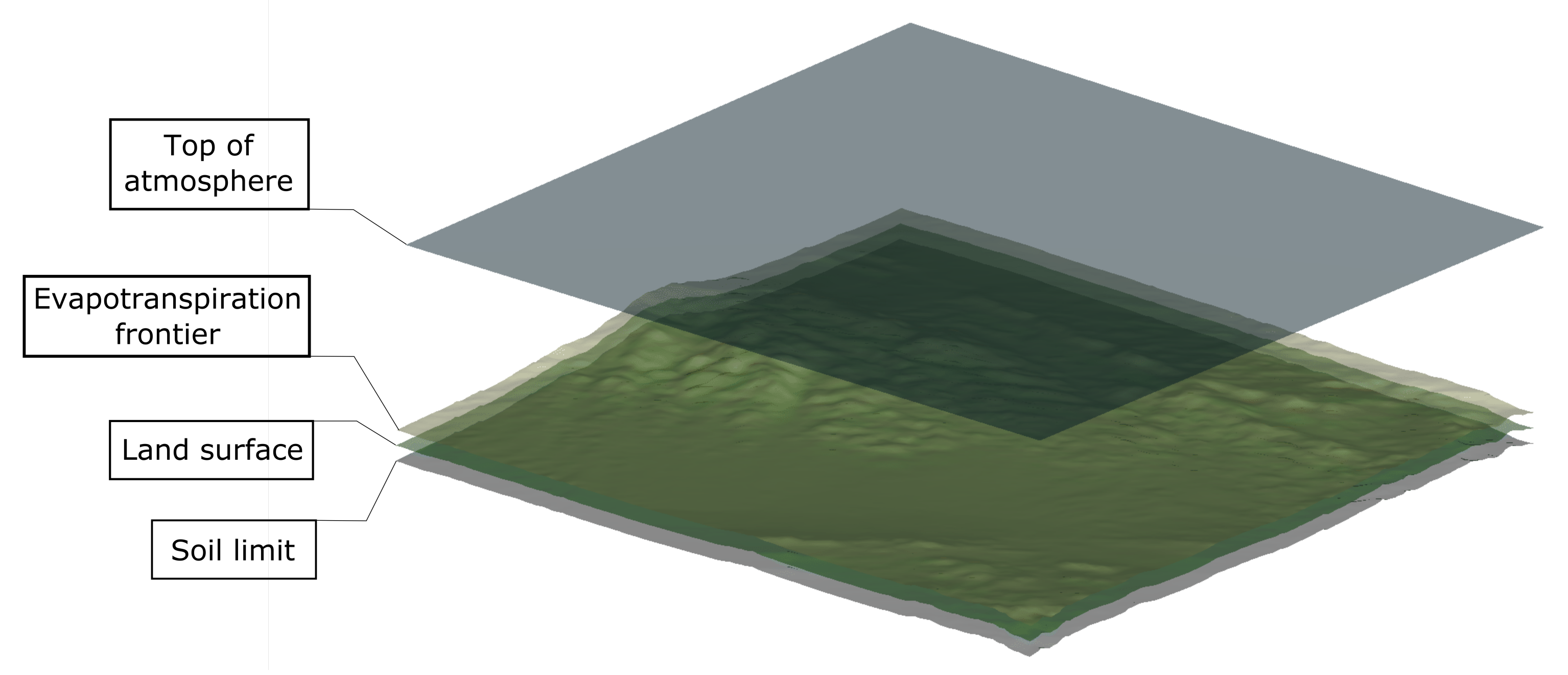
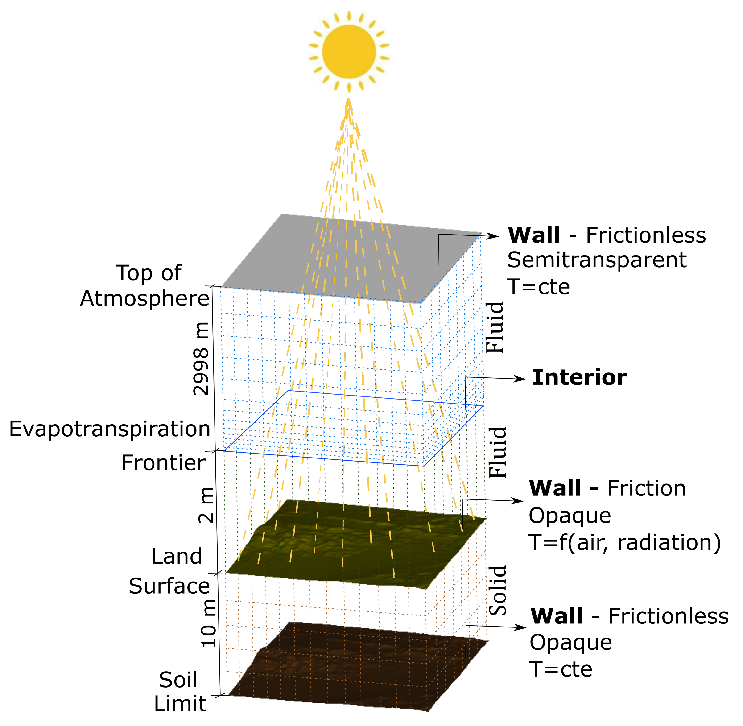
2. Geometric Model
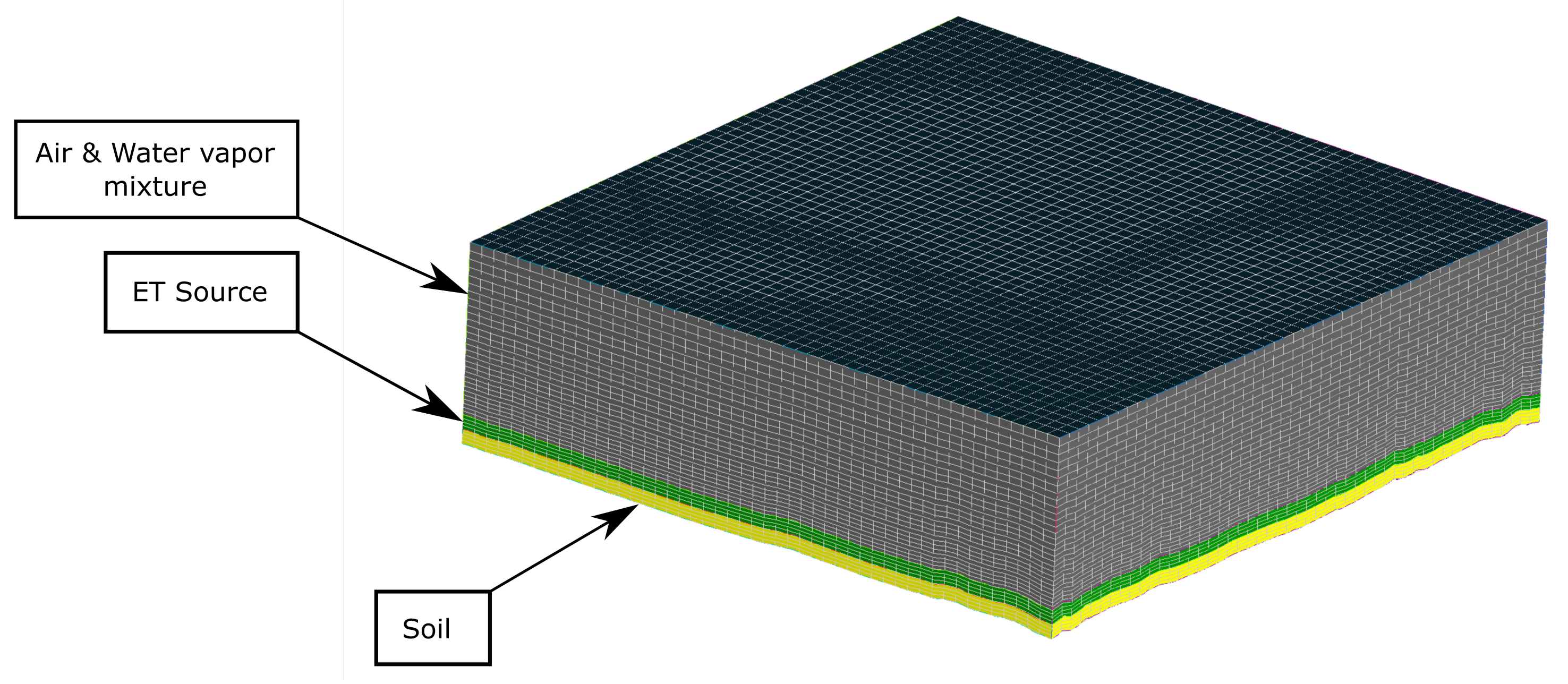
3. Numerical CFD Model
3.1. Theoretical Model
3.2. Simulation Methodology
3.3. Boundary Conditions
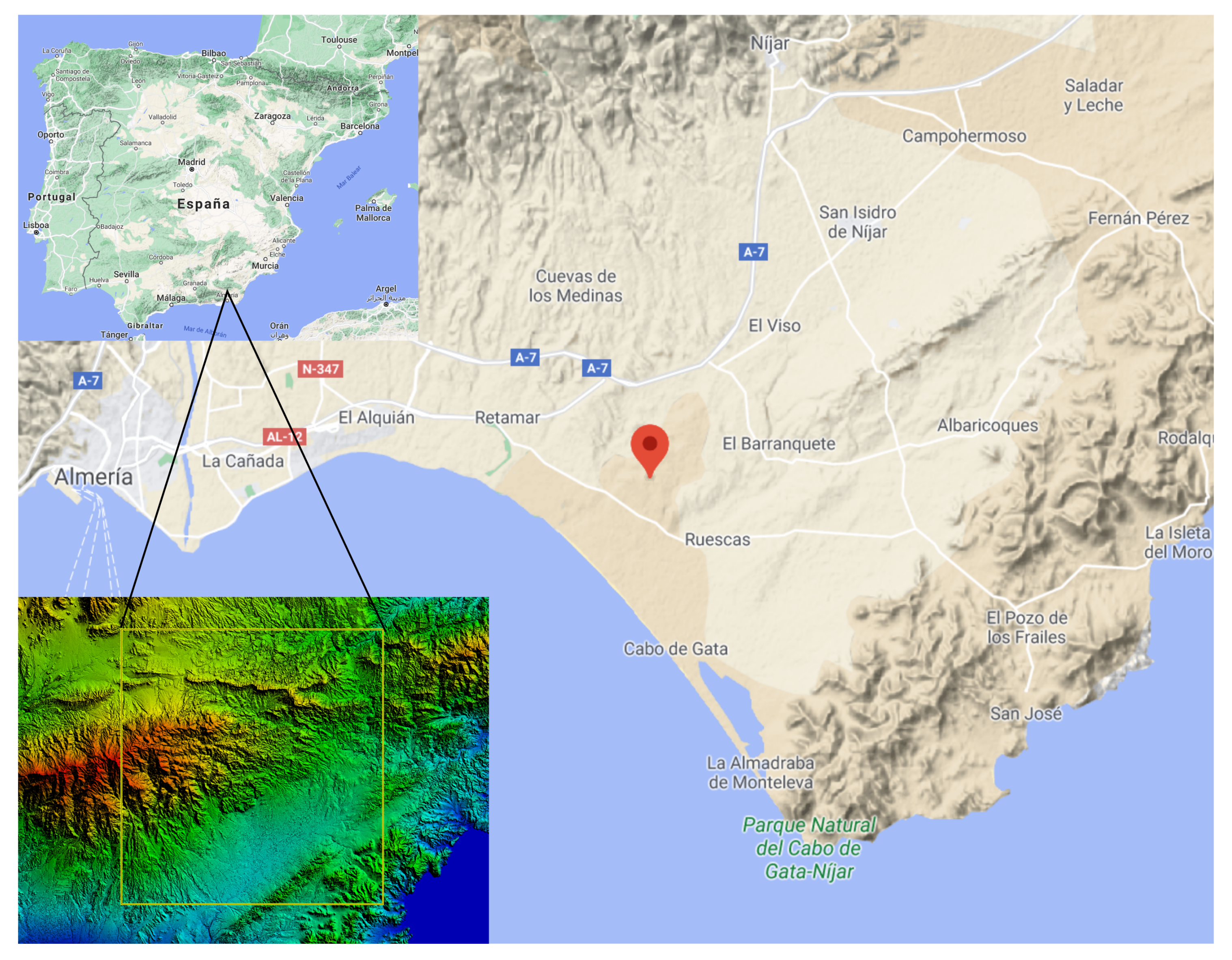
4. Example of Use: Cabo de Gata
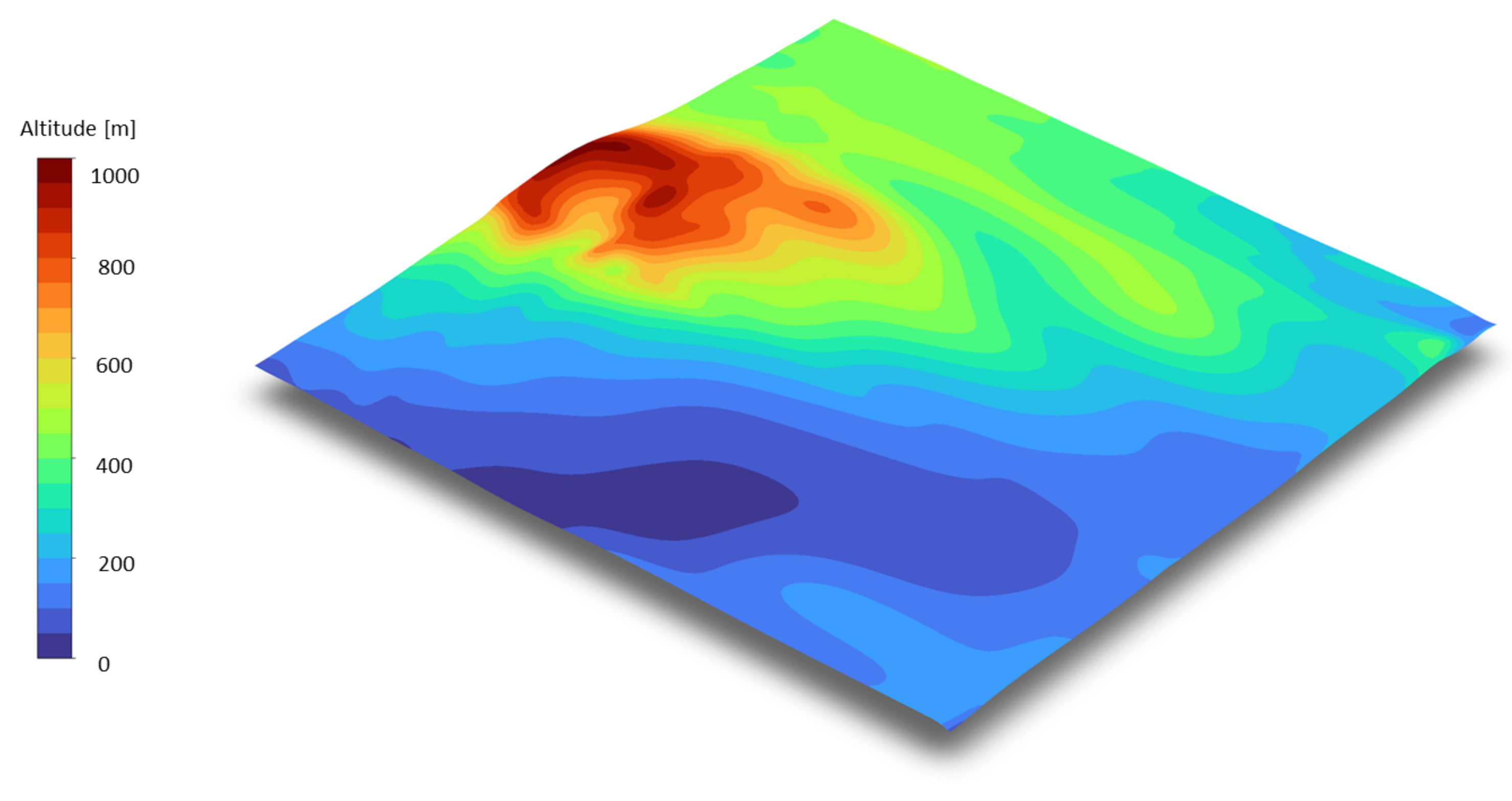
4.1. Study Area
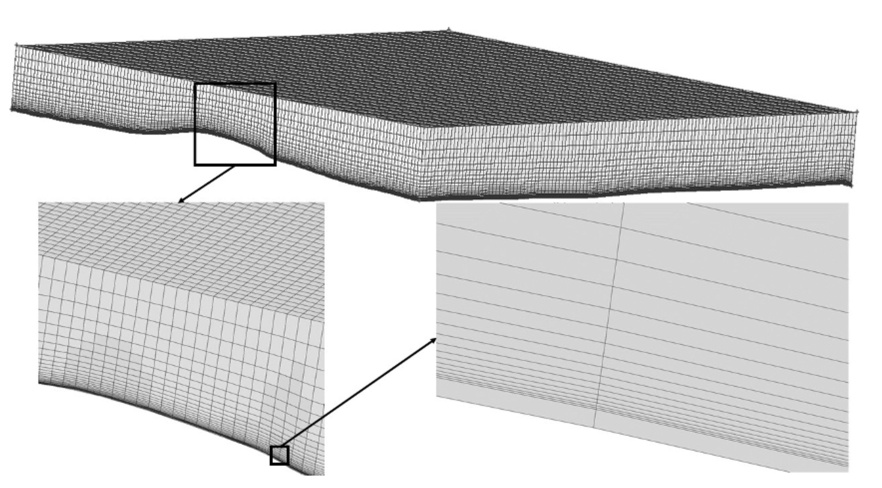
4.2. Geometric and Numerical Model
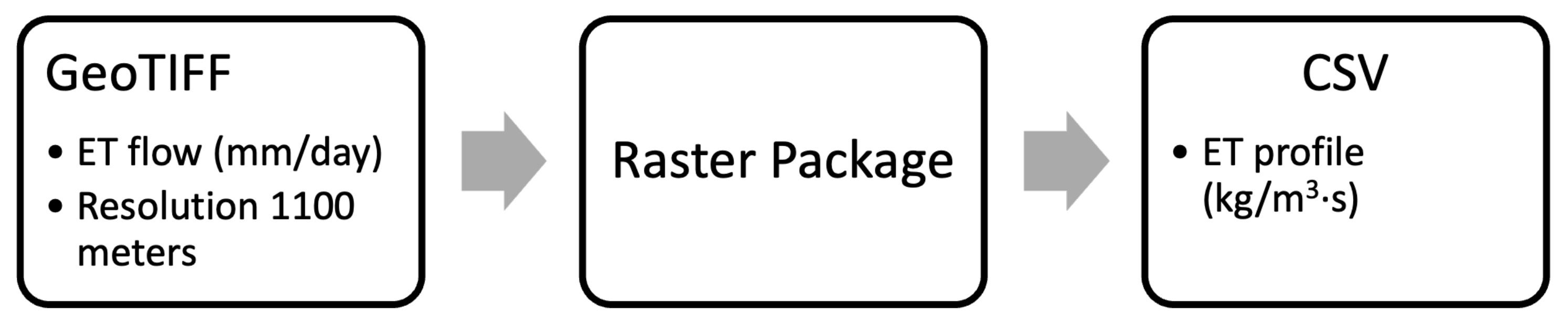
4.3. Input Data
4.4. Simulation Methodology
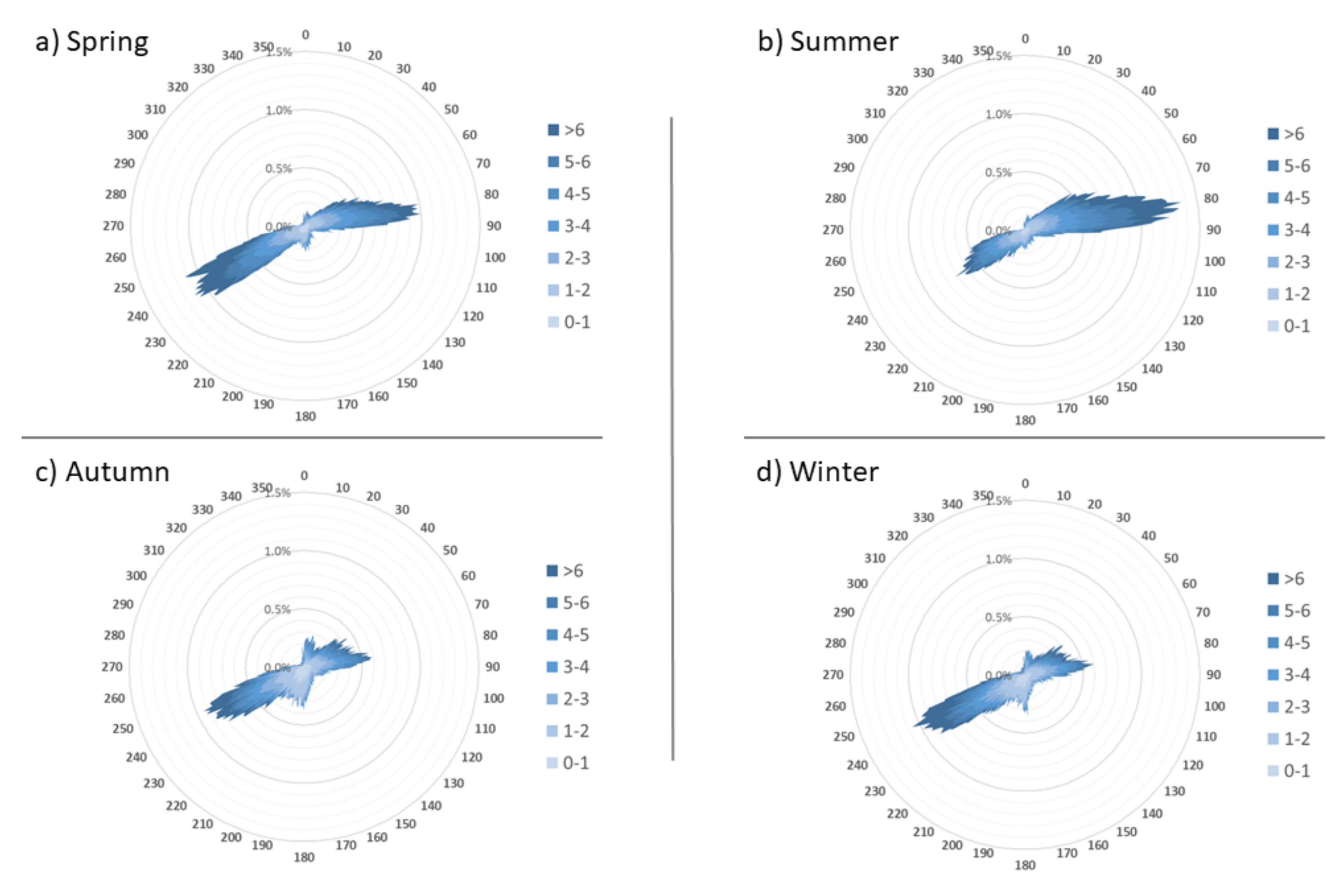
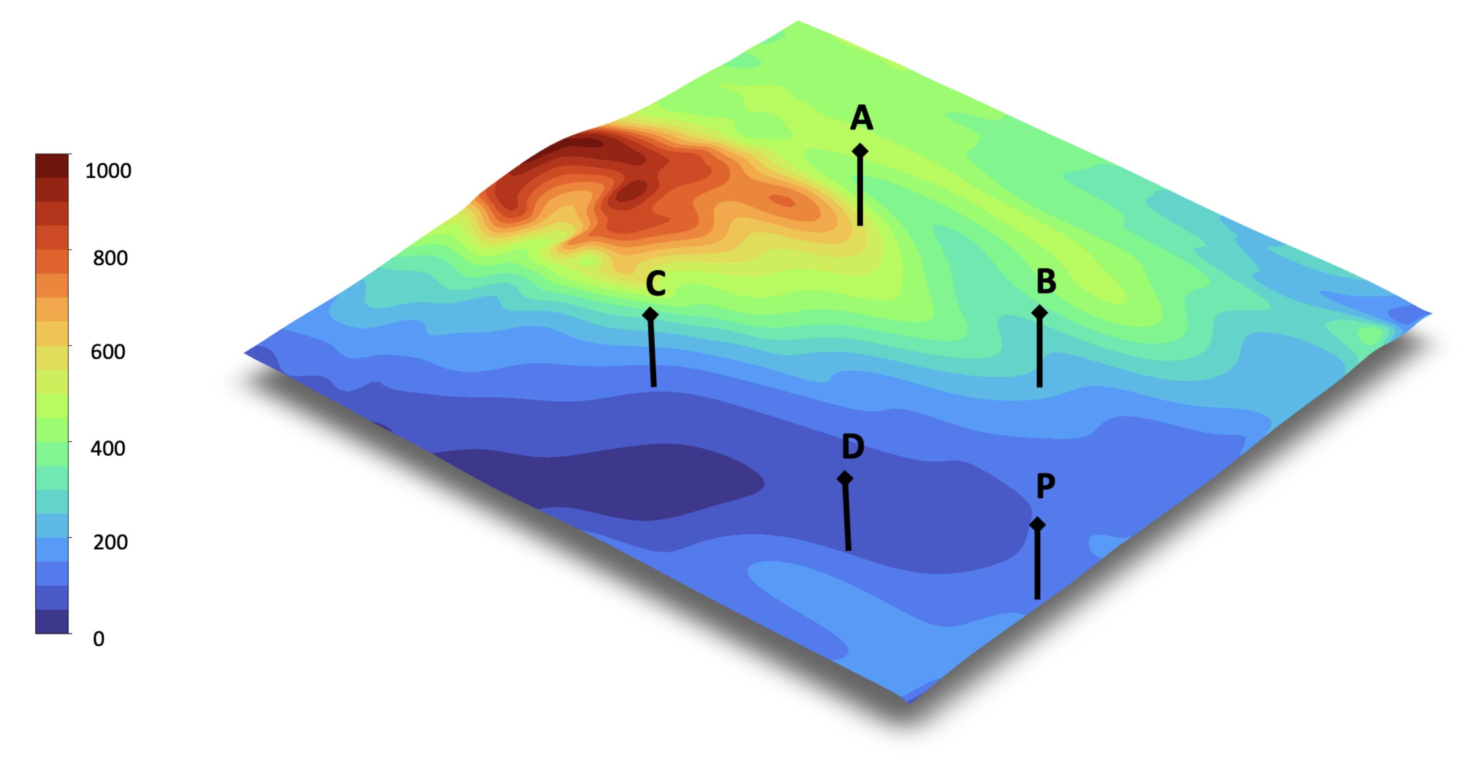
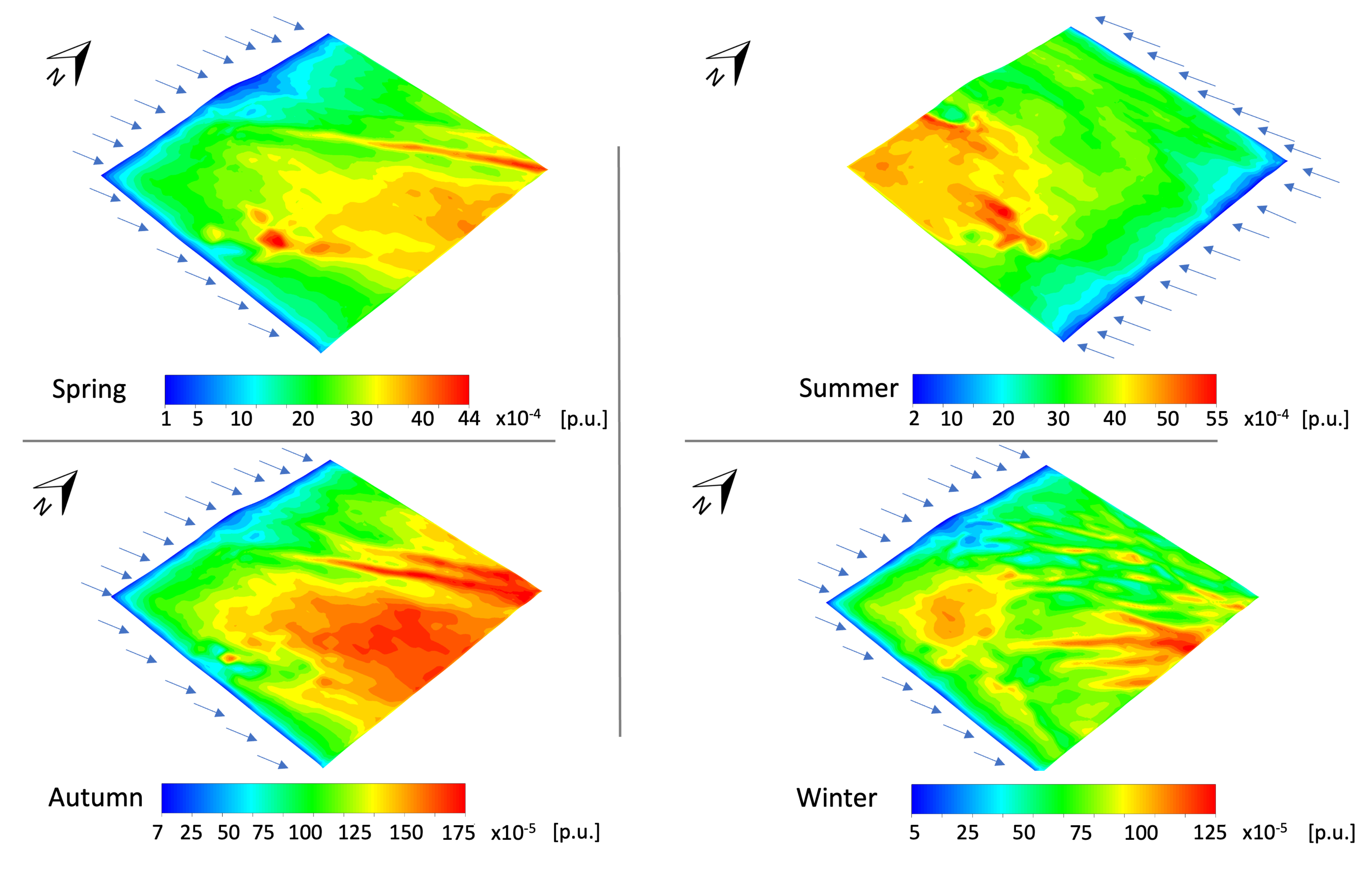
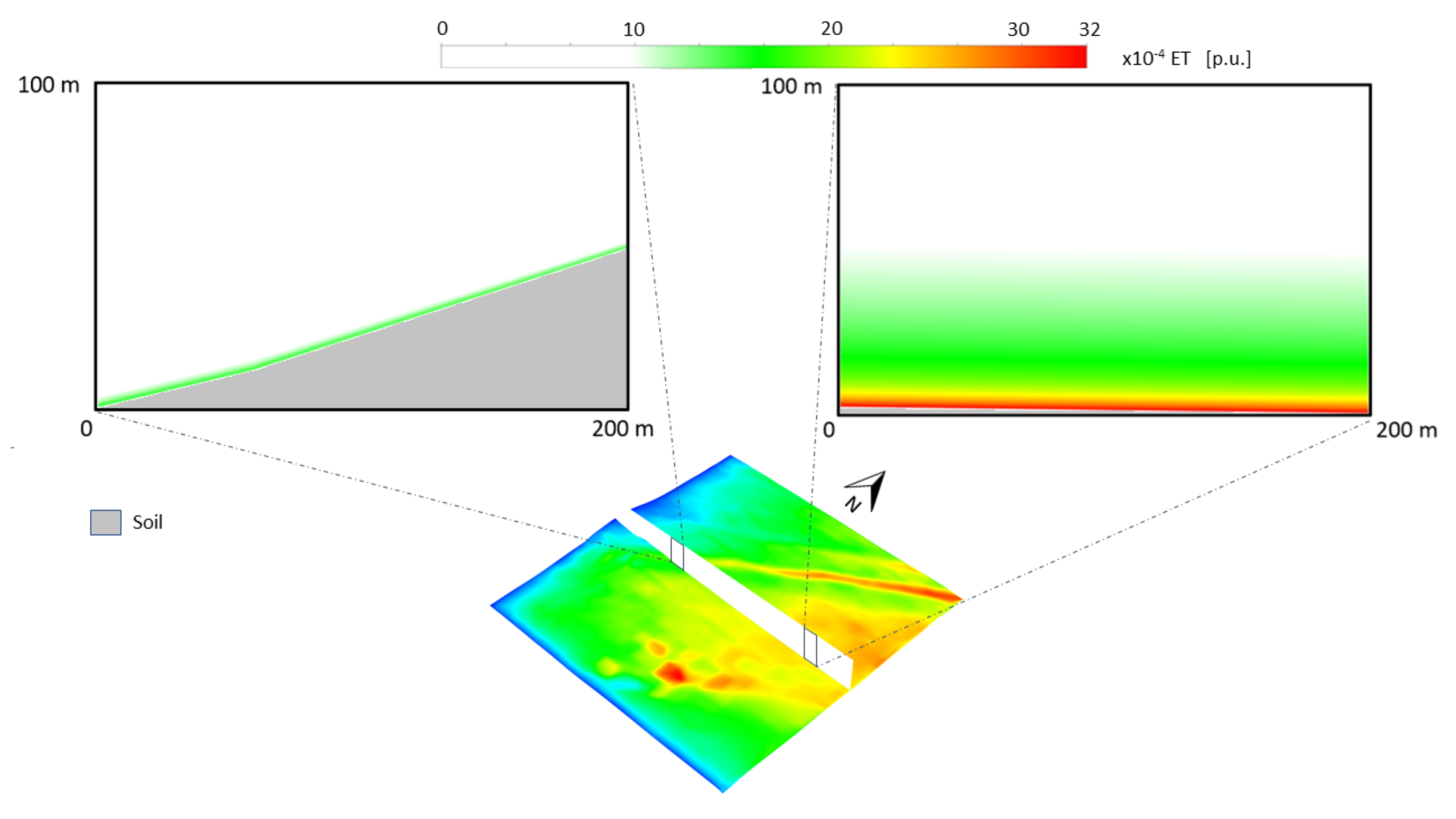
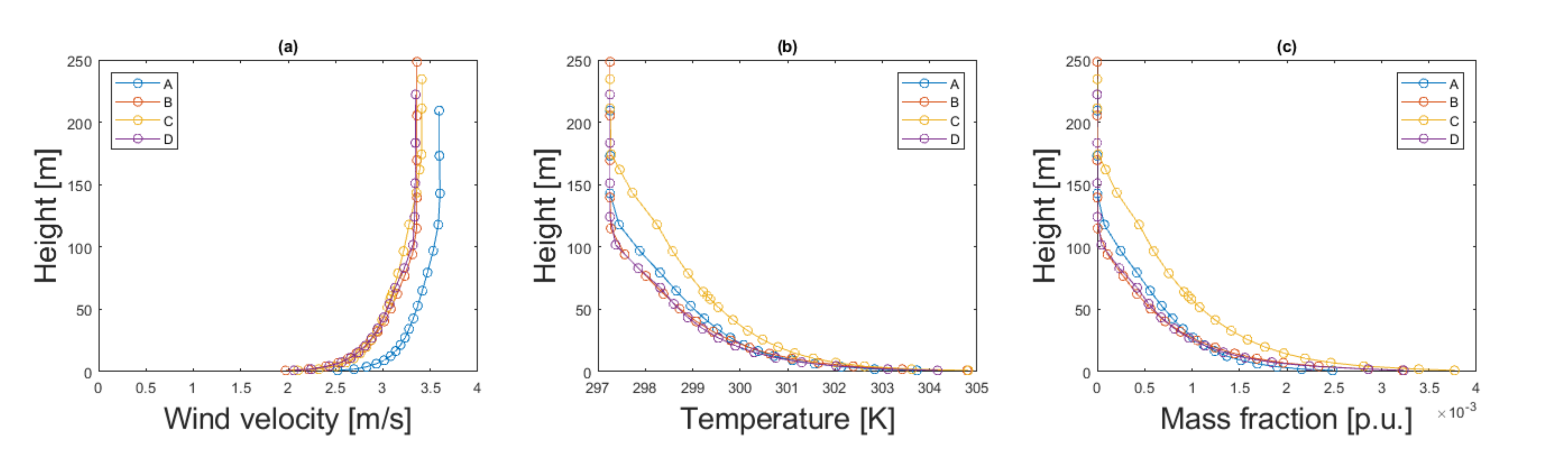
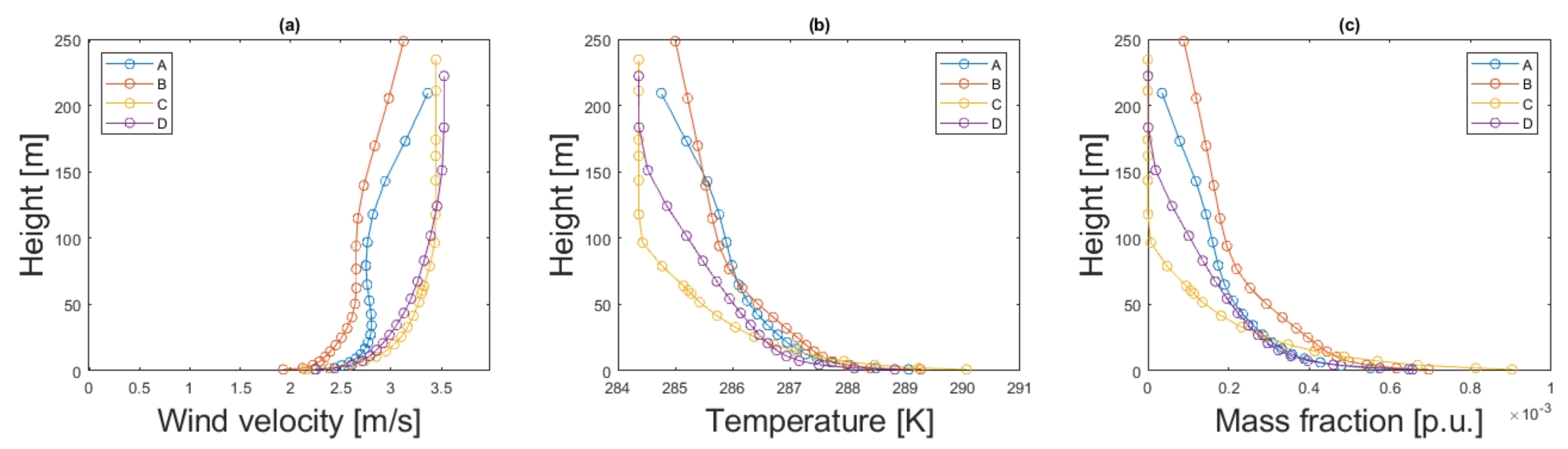
4.5. Results
5. Conclusions
Author Contributions
Funding
Institutional Review Board Statement
Informed Consent Statement
Data Availability Statement
Acknowledgments
Conflicts of Interest
References
- United Nations Framework Convention on Climate Change. Adoption of the Paris Agreement. In Proceedings of the Conference of the Parties on Its Twenty-First Session, Paris, France, 30 November–13 December 2015; p. 32.
- Cheng, X.; Mao, H.; Ni, J. Numerical prediction and CFD modeling of relative humidity and temperature for greenhouse-crops system. Nongye Jixie Xuebao Trans. Chin. Soc. Agric. Mach. 2011, 42, 157, 173–179. [Google Scholar]
- Roy, J.C.; Pouillard, J.B.; Boulard, T.; Fatnassi, H.; Grisey, A. Experimental and CFD results on the CO2distribution in a semi closed greenhouse. Acta Hortic. 2014, 1037, 993–1000. [Google Scholar] [CrossRef]
- Kichah, A.; Bournet, P.E.; Migeon, C.; Boulard, T. Measurement and CFD simulation of microclimate characteristics and transpiration of an Impatiens pot plant crop in a greenhouse. Biosyst. Eng. 2012, 112, 22–34. [Google Scholar] [CrossRef]
- Bouhoun Ali, H.; Bournet, P.E.; Danjou, V.; Morille, B.; Migeon, C. CFD simulations of the night-time condensation inside a closed glasshouse: Sensitivity analysis to outside external conditions, heating and glass properties. Biosyst. Eng. 2014, 127, 159–175. [Google Scholar] [CrossRef]
- Maher, D.; Hana, A. CFD investigation of temperature distribution, air flow pattern and thermal comfort in natural ventilation of building using solar chimney. World J. Eng. 2020, 17, 78–86. [Google Scholar] [CrossRef]
- Catalina, T.; Virgone, J.; Kuznik, F. Evaluation of thermal comfort using combined CFD and experimentation study in a test room equipped with a cooling ceiling. Build. Environ. 2009, 44, 1740–1750. [Google Scholar] [CrossRef]
- Albatayneh, A.; Alterman, D.; Page, A. Adaptation the Use of CFD Modelling for Building Thermal Simulation; ACM International Conference Proceeding Series; Association for Computing Machinery: New York, NY, USA, 2018; pp. 68–72. [Google Scholar] [CrossRef]
- Gkatsopoulos, P. A Methodology for Calculating Cooling from Vegetation Evapotranspiration for Use in Urban Space Microclimate Simulations. Procedia Environ. Sci. 2017, 38, 477–484. [Google Scholar] [CrossRef]
- Gromke, C.; Blocken, B.; Janssen, W.; Merema, B.; van Hooff, T.; Timmermans, H. CFD analysis of transpirational cooling by vegetation: Case study for specific meteorological conditions during a heat wave in Arnhem, Netherlands. Build. Environ. 2015, 83, 11–26. [Google Scholar] [CrossRef]
- Dimoudi, A.; Nikolopoulou, M. Vegetation in the urban environment: Microclimatic analysis and benefits. Energy Build. 2003, 35, 69–76. [Google Scholar] [CrossRef] [Green Version]
- Szucs, A.; Moreau, S.; Allard, F. Aspects of stadium design for warm climates. Build. Environ. 2009, 44, 1206–1214. [Google Scholar] [CrossRef]
- Vidal-López, P.; Martínez-Alvarez, V.; Gallego-Elvira, B.; Martín-Górriz, B. Determination of synthetic wind functions for estimating open water evaporation with Computational Fluid Dynamics. Hydrol. Process. 2012, 26, 3945–3952. [Google Scholar] [CrossRef]
- Ashie, Y.; Kono, T. Urban-scale CFD analysis in support of a climate-sensitive design for the Tokyo Bay area. Int. J. Climatol. 2011, 31, 174–188. [Google Scholar] [CrossRef]
- Helman, D.; Givati, A.; Lensky, I.M. Annual evapotranspiration retrieved from satellite vegetation indices for the eastern Mediterranean at 250 m spatial resolution. Atmos. Chem. Phys. 2015, 15, 12567–12579. [Google Scholar] [CrossRef] [Green Version]
- Helman, D.; Osem, Y.; Yakir, D.; Lensky, I.M. Relationships between climate, topography, water use and productivity in two key Mediterranean forest types with different water-use strategies. Agric. For. Meteorol. 2017, 232, 319–330. [Google Scholar] [CrossRef]
- Helman, D.; Lensky, I.M.; Yakir, D.; Osem, Y. Forests growing under dry conditions have higher hydrological resilience to drought than do more humid forests. Glob. Chang. Biol. 2017, 23, 2801–2817. [Google Scholar] [CrossRef]
- Helman, D.; Bonfil, D.J.; Lensky, I.M. Crop RS-Met: A biophysical evapotranspiration and root-zone soil water content model for crops based on proximal sensing and meteorological data. Agric. Water Manag. 2019, 211, 210–219. [Google Scholar] [CrossRef]
- Helman, D.; Lensky, I.M.; Bonfil, D.J. Early prediction of wheat grain yield production from root-zone soil water content at heading using Crop RS-Met. Field Crop. Res. 2019, 232, 11–23. [Google Scholar] [CrossRef]
- Dahm, C.N.; Cleverly, J.R.; Allred Coonrod, J.E.; Thibault, J.R.; McDonnell, D.E.; Gilroy, D.J. Evapotranspiration at the land/water interface in a semi-arid drainage basin. Freshw. Biol. 2002, 47, 831–843. [Google Scholar] [CrossRef]
- García, M.; Sandholt, I.; Ceccato, P.; Ridler, M.; Mougin, E.; Kergoat, L.; Morillas, L.; Timouk, F.; Fensholt, R.; Domingo, F. Actual evapotranspiration in drylands derived from in-situ and satellite data: Assessing biophysical constraints. Remote Sens. Environ. 2013, 131, 103–118. [Google Scholar] [CrossRef]
- Morillas, L.; Villagarcía, L.; Domingo, F.; Nieto, H.; Uclés, O.; García, M. Environmental factors affecting the accuracy of surface fluxes from a two-source model in Mediterranean drylands: Upscaling instantaneous to daytime estimates. Agric. For. Meteorol. 2014, 189–190, 140–158. [Google Scholar] [CrossRef]
- Raithby, G.D.; Chui, E.H. A Finite-Volume Method for Predicting a Radiant Heat Transfer in Enclosures with Participating Media. J. Heat Transf. 1990, 112, 415–423. [Google Scholar] [CrossRef]
- Launder, B.E.; Spalding, D.B. The numerical computation of turbulent flows. Comput. Methods Appl. Mech. Eng. 1974, 3, 269–289. [Google Scholar] [CrossRef]
- Zheng, S.; Zhao, L.; Li, Q. Numerical simulation of the impact of different vegetation species on the outdoor thermal environment. Urban For. Urban Green. 2016, 18, 138–150. [Google Scholar] [CrossRef]
- Launder, B.E.; Spalding, D.B. MAN—ANSYS Fluent User’ s Guide Release 15.0. Knowl. Creat. Diffus. Util. 2013, 15317, 724–746. [Google Scholar]
- Soutullo, S.; Sánchez, M.N.; Enríquez, R.; Jimenez, M.J.; Heras, M.R. Empirical estimation of the climatic representativeness in two different areas: Desert and Mediterranean climates. Energy Procedia 2017, 122, 829–834. [Google Scholar] [CrossRef]
- Flóvenz, O.; Hersir, G.P.; Sæmundsson, K.; Ármannsson, H.; Friethriksson, T. Geothermal energy exploration techniques. In Comprehensive Renewable Energy; Elsevier: Amsterdam, The Netherlands, 2012; Volume 7, pp. 51–95. [Google Scholar] [CrossRef]
- Hijmans, R. Package ’Raster’ Type Package Title Geographic Data Analysis and Modeling. 2021. Available online: https://cran.r-project.org/web/packages/raster/raster.pdf (accessed on 30 January 2022).


| Temperature | Soil Temperature | Humidity | Wind Speed | Wind Angle | Radiation | |
|---|---|---|---|---|---|---|
| °C | °C | % | m·s−1 | Azimut | W·m | |
| Spring | 17.45 | 17.15 | 63.61 | 3.42 | 240° | 537.77 |
| Summer | 24.26 | 23.96 | 64.66 | 3.32 | 80° | 545.25 |
| Autumn | 15.91 | 15.61 | 72.16 | 2.65 | 240° | 371.46 |
| Winter | 11.36 | 11.06 | 70.95 | 2.93 | 240° | 372.65 |
Publisher’s Note: MDPI stays neutral with regard to jurisdictional claims in published maps and institutional affiliations. |
© 2022 by the authors. Licensee MDPI, Basel, Switzerland. This article is an open access article distributed under the terms and conditions of the Creative Commons Attribution (CC BY) license (https://creativecommons.org/licenses/by/4.0/).
Share and Cite
Fernández-Pacheco, V.M.; Antuña-Yudego, E.; Carús-Candás, J.L.; Suárez-López, M.J.; Álvarez-Álvarez, E. An Evapotranspiration Evolution Model as a Function of Meteorological Variables: A CFD Model Approach. Sustainability 2022, 14, 3800. https://doi.org/10.3390/su14073800
Fernández-Pacheco VM, Antuña-Yudego E, Carús-Candás JL, Suárez-López MJ, Álvarez-Álvarez E. An Evapotranspiration Evolution Model as a Function of Meteorological Variables: A CFD Model Approach. Sustainability. 2022; 14(7):3800. https://doi.org/10.3390/su14073800
Chicago/Turabian StyleFernández-Pacheco, Víctor Manuel, Elena Antuña-Yudego, Juan Luis Carús-Candás, María José Suárez-López, and Eduardo Álvarez-Álvarez. 2022. "An Evapotranspiration Evolution Model as a Function of Meteorological Variables: A CFD Model Approach" Sustainability 14, no. 7: 3800. https://doi.org/10.3390/su14073800
APA StyleFernández-Pacheco, V. M., Antuña-Yudego, E., Carús-Candás, J. L., Suárez-López, M. J., & Álvarez-Álvarez, E. (2022). An Evapotranspiration Evolution Model as a Function of Meteorological Variables: A CFD Model Approach. Sustainability, 14(7), 3800. https://doi.org/10.3390/su14073800