Abstract
A well-thought-out strategy for shaping the transport of the future is a challenge for countries and integration groups. The answer to which modes of transport should become a priority in the context of incurred and planned investments should largely depend on their observed and forecasted environmental impact. This paper focuses on the scope and content of EU macro-regional strategies. The main objectives of the study were to identify common assumptions and differences between the Adriatic and Ionian Region and the Baltic Sea Region in terms of sustainable transport and provide a critical assessment of the EU Strategy for the Adriatic and Ionian Region (EUSAIR) and the EU Strategy for the Baltic Sea Region (EUSBSR) compliance with the assumptions of the White Paper on Transport, as well as the attempt to answer the question of which modes of transport should be prioritized by the analyzed macro-regions, making transport decarbonization one of their main goals. It is possible to state that the assumptions of both the strategies of the macro-regions seem to be partially consistent with the White Paper on Transport vision. However, the emphasis of the macro-regions on the development of maritime transport is somewhat omitted in the White Paper. Among the countries of both areas (EUSAIR, EUSBSR), estimates showed a statistically significant (p < 0.05) positive impact on the volume of loads transported by road transport. An increase in the volume loads by 1% resulted in an increase in air pollution by 0.446% (EUSAIR) and 0.728% (EUSBSR). The elasticity of air pollution, regarding loads’ road transport changes, was the highest compared to other transport modes in the studied areas. This proves the highest emissivity of road transport. In the EUSAIR countries, an increase by 1% of the volume of transport by railway resulted in a decrease in air pollution, with emissions of greenhouse gases decreasing by 0.063%. Considering the analyzed documentation, reports, strategies, and assumptions, it seems right to clearly emphasize the role of rail transport in the decarbonization of transport. According to the authors, mainly, this branch of transport can significantly reduce the emission of gases into the atmosphere and thus contribute to the so-called “green deal”. However, many activities must be undertaken for this to happen, not only investment ones. First of all, it is worth paying attention to the coherence of regional strategies with the European transport development plan contained in the White Paper.
1. Introduction
Transport is responsible for a quarter of Europe’s greenhouse gas (GHG) emissions. There is increasing public debate about the environmental impact of different transport modes and their potential impact on improving the cleanliness of the environment. One of the significant challenges facing the European Union (EU) is the reduction of greenhouse gas emissions, which justifies the actions taken in this area at the community level. An essential activity in this respect was the adoption of the European Strategy for Low-Emission Mobility. Its main priorities are:
- increasing the efficiency of the transport system;
- speeding up the deployment of low-emission alternative energy for transport;
- moving towards zero-emission vehicles [1].
The initiative of the EU in the indicated scope should be appreciated. Nevertheless, it seems extremely important to look critically at international institutions’ strategies, action plans, and integration groups associating individual countries and regions.
EU macro-regional strategies are a form of transnational cooperation whose primary goal is to solve critical problems across national borders. This type of cooperation, especially in broadly understood environmental protection, is nothing new. Many cooperative endeavors were initiated in large transnational areas covering multiple countries between the 1950s and the 1970s, and the EU has funded such cooperation since 1997 [2] as part of the so-called ‘Strand B’ of INTERREG. It should be noted that the main challenges faced by the initiators of this type of action are ensuring consistency with other guidelines, a high level of detail of planned activities, and ensuring the highest possible probability of achieving the assumed goals. An example of a vital document in this context is the White Paper on Transport, a comprehensive strategy for a competitive transport system. The compliance of the EU macro-regional strategies’ assumptions with such documents seems necessary to achieve the assumed development and environmental goals.
This paper focuses on the scope and content of EU macro-regional strategies. The strategies of two macro-regions were analyzed: the Baltic Sea Region (EUSBSR) and the Adriatic and Ionian Region (EUSAIR). These macro-regions were deliberately selected due to several factors, the most important of which are a similar population potential, access to the sea, similarly formulated main goals in macro-regional strategies, and a similar distribution of investments, with the dominance of expenditure on railways. After a short overview of the most critical assumptions of both strategies, common objectives focused around the pillar of connecting the region were identified. Therefore, the aims of this study include:
- identifying common assumptions and differences between the EUSAIR and the EUSBSR in terms of sustainable transport;
- critical assessment of EUSAIR and EUSBSR compliance with the assumptions of the White Paper on Transport;
- attempting to answer the question of which modes of transport should be prioritized by the analyzed macro-regions, making environmental protection one of their main goals.
The paper presents the results of the analysis of selected legal acts in terms of the diagnosis of their consistency level. The analysis of statistical data characterizing the level of greenhouse gas emissions in transport, the volume and structure of transport in the EUSAIR and EUSBSR countries, and the amount of investment in individual modes of transport was performed. Moreover, an attempt was made to diagnose the linear relationships between expenditure on priority programs of the CEF (Connecting Europe Facility) instrument, expenditure on individual modes of transport, and the amount of transport for the modes mentioned above.
The new approach presented in the article includes aspects concerning, among other things:
- -
- analysis and evaluation of the coherence of several policies, i.e., macro-regional strategies, White Paper on Transport, EU funds spending under CEF;
- -
- the allocation of EU CEF funds and the coherence of these investments with the strategies of macro-regions;
- -
- verification of the correlation of investments with CEF and the volume of transport in individual countries and macro-regions;
- -
- isolation of rail transport as the one with the most considerable invested resources and omitted in the strategies of macro-regions;
- -
- an indication of differences between the strategies of macro-regions and the White Paper on Transport;
- -
- identifying gaps in EU action in the context of transport decarbonization;
- -
- verification of policy assumptions with reality.
The paper’s novelty may constitute a significant contribution to the literature and may also be treated as a form of recommendation for regulatory institutions or bodies preparing regional development strategies. So far, no work has been completed on a document that is an analysis of the coherence of the macro-regions’ strategies and the White Paper on Transport.
The structure of the paper is as follows: state of the art and methodology (2), the general concept of macro-regions (3), technical aspects of transportation in the macro-regions and the TEN-T (Trans-European Transport Network) structure in them, as well as the volume and size of transport (4), conclusions (5).
2. State of the Art and Methodology
Various modes of transport in climate change are a relatively popular research issue. Scientific publications on environmental pollution by road transport play an important role here. Interesting conclusions can be drawn from the study in Ref. [3], whose authors analyzed the influencing factors of road transport carbon emissions from the perspective of the “human-vehicle-environment”. The investigation data of Chongqing Transportation Group, passenger transport emissions, were used to carry out a stepwise regression analysis. The results of the conducted research showed that the most significant impact on the level of greenhouse gas emissions in road passenger transport relates to factors such as the type of oil used, the driving mileage of the secondary trunk road, and the vehicle’s service life. On the other hand, the driving age, driving mileage of the main trunk road, and the highway are not the main influencing factors.
An interesting topic in the literature is the relationship between economic growth, energy consumption, and greenhouse gas emissions in road transport. In this context, an example of an interesting research initiative is in the study of Ref. [4]. The authors attempted to understand the vital, relevant factors influencing energy consumption and energy-related emissions in Thailand’s road passenger transport. The growth in emissions was lower than energy consumption by around 1.38 times between 2007 and 2017, which should be linked to biofuels promotion in Thailand. The same study also took up the interesting topic of reducing greenhouse gas (GHG) emissions due to the economic slowdown. Considerations on this topic have also recently been undertaken in the context of the slowdown caused by the global COVID-19 pandemic [5].
The significant share of road transport in total greenhouse gas emissions increases interest in this issue, leading to modeling attempts and developing future scenarios. In this context, it is worth paying attention to, inter alia, the study in Ref. [6], which attempted a detailed analysis of the GHG emissions in four European countries due to different types of road transport vehicles. The added value of the discussed study was the development of several recommendations in fuel efficiency policies, city traffic management, digital technologies, investments for low-emission mobility, and efficient pricing policies in transport. The study also provides interesting conclusions [7] and attempts to model road transport emissions in Germany in 2040. It highlights the importance of behavioral changes in passenger transport, especially in urban areas, which must be paralleled by technological measures to increase societal benefits. According to the modeling results concerning freight transport, the additional reduction in traffic emissions comes to 90% from technological measures, i.e., the electrification of long-distance trucking.
Research carried out in Great Britain shows the great importance of road transport in polluting the natural environment. According to the data presented in the study [8], although the highest levels of road pollution are localized, low levels of road pollution are generally ubiquitous. The authors of the study stated that, although roads occupy an estimated 0.8% of the area of Great Britain, their zone of influence covers 70% of the country’s area. Only about 6% of the area can escape any impact of road transport pollutants.
The literature on the subject also includes studies dealing with the issue of the impact of air transport on the environment. One of the most recent is the work of Calderon-Tellez and Herrera [9], in which the authors attempted to assess the impact of air transport on the environment, taking into account the changes caused by the COVID-19 pandemic. The simulations showed how difficult it is to reconcile the public interest related to the need to move with attempts to reduce the number of air traffic connections to improve the cleanliness of the environment.
It is also worth paying attention to studies on the specific competition between air and rail transport, especially high-speed, regarding their potential impact on the environment. At this point, it is worth referring to the study by D’Alfonso et al. [10], in which the authors indicated some negative environmental consequences of competition between these modes of transport, stressing, among other things, that railways can be competitive to air transport only when using high speeds, which, however, increases their emissivity.
High-speed rail and environmental pollution are relatively popular research topics. For example, in a study [11], attention was focused on the impact of high-speed rail accessibility on haze pollution in China. The impact of high-speed rail on air pollution in China was also discussed in Ref. [12]. According to the estimation results, carbon monoxide, one of the primary sources of pollution from cars, was reduced by 0.047 mg/m3 (4.3% of the mean) in the vicinity of highways where high-speed lines were built compared to areas not affected by the HSR. The topic of the beneficial impact of railways on the condition of the natural environment was also discussed in other studies [13,14]. It is also worth referring to the publication [15] that deals with the economic and environmental impact of the new Mediterranean Rail Corridor in Andalusia. The authors of the publication emphasized how positive the economic impact of this infrastructure is and how the environmental benefits outweigh economic ones. The economic benefits from the development of rail transport were also emphasized in the study [16].
Studies dealing with maritime transport should not be omitted in considering the impact of various modes of transport on the environment. A study [17] is worth mentioning here that focused on the methodological aspects of modeling environmental pollution in maritime transport. Another study [18] also contributes to this knowledge, addressing for the first time the impact of maritime transport on the economy and the level of environmental pollution in France. It is worth emphasizing that the study results by the cited authors are rather critical towards maritime transport, indicating a low potential for creating new jobs and a high position of this industry in the ranking of those that pollute the natural environment the most. However, the authors’ awareness of the discussed study regarding certain methodological limitations should be appreciated. They are related to, among other things, long and global logistic supply chains of other industries, consuming intermediate services of transport that were not visible in the domestic input–output framework.
The impact of maritime transport on climate change has also been discussed in other studies [19,20,21,22]. The literature on the subject also includes studies on maritime transport in the context of environmental protection and the so-called green shipping [23,24,25,26,27].
As emphasized in the introduction, EU macro-regional strategies are a form of transnational cooperation whose primary goal is to solve critical problems, such as environmental protection, across national borders. Considering the research problem of this paper, it is worth referring here to the study [2] that deals with the role of environmental issues in the adoption processes of EU macro-regional strategies. Notably, the article referred to, among others, the EU strategy for the Baltic Sea Region and Adriatic and Ionian Region. One of the leading research inspirations is a rather critical assessment of macro-regional strategies in terms of their potential impact on the improvement of the natural environment, which the authors made of the discussed publication. The key research challenge in this context is to make, as comprehensively as possible, an assessment of the EU strategy for the selected macro-regions in terms of the environmental impact protection of various modes of transport.
The literature on the subject includes studies presenting the research results on the impact of specific modes of transport on the environment of the Adriatic and Ionian Region [28,29] and the Baltic Sea Region [30,31].
As mentioned earlier, one of the main challenges for EU macro-regional strategy makers is to ensure their compatibility with other programs and guidelines. In this context, a fundamental research issue seems to be the compliance of the EU macro-regional strategies with the objectives of the Trans-European Transport Network (TEN-T) and the White Paper on Transport. Of course, among the most recent scientific studies, there is no shortage of publications assessing the overall concept of the TEN-T [32,33,34,35,36], analytical studies on specific corridors and selected countries [37,38], as well as studies assessing environmental and safety impacts of the TEN-T [39]. The literature on the subject also includes studies on sustainable transport and scientific papers analyzing the main goals and assumptions of the White Paper on Transport [40,41]. However, comparing the EU strategies of selected macro-regions and the assumptions of the TEN-T and White Paper on Transport seem to remain somewhat out of research interests, which prompts the authors of this study to attempt to fill this knowledge gap.
As for the research methods used in the article, refer to the analysis typical of policy and strategy evaluation. In this case, they are:
- -
- a method of analysis and criticism of the literature: its essence consists of adapting a new problem to the existing knowledge. It is done by analyzing and criticizing the literature on the subject. It is about showing the similarities, differences, relationships, dependencies, and features necessary in scientific theories, in hypotheses and assumptions, in ideas of action, and views on the world;
- -
- statistical method: the research consists of concluding the prominent features of sets of statistical elements. It is mainly about two types of problems that require statistical analysis: searching for means or deviations in an ordered number of observations regarding a given variable feature and research leading directly to obtaining correlation coefficients, i.e., the interdependence of two or more studies on causal relationships phenomena (processes).
- -
- panel data regression models: econometric analysis aimed to assess the significance and influence direction of the volume of freight transport (broken down through transport on the amount of air pollution with greenhouse gases). To compare EUSAIR to EUSBSR area in terms of transport impact on greenhouse gas emissions, two-panel data models (NEUSAIR = 4, NEUSBSR = 8, T = 2005–2019) were constructed and estimated. The authors’ use of regression methods was inspired, inter alia, by the work of Castellano et al. [42].
3. General Concept of Macro-Regions: EUSAIR & EUSBSR
It is the EU that initiated creating strategies for macro-regions. They were requested by EU and non-EU Member States located in the same geographical area via the European Council. Its aim is to deal with everyday challenges and opportunities identified in each macro-region. As intergovernmental initiatives, the implementation relies on the commitment of the participating countries. There are four macro-regions and strategies adopted so far by the EU: the EU Strategy for the Baltic Sea Region (2009), the Danube Region (2010), the Adriatic and Ionian Region (2014), and the Alpine Region (2015). The four EU macro-regions encompass 27 countries (Figure 1) with more than 340 million people, while the European Commission plays a leading role in the strategic coordination of the strategy’s key delivery stages. It supports key actors and evaluates and reports on the macro-regional strategies to guarantee the EU dimension. To succeed, the EU macro-regional strategies need a balance between the leadership provided by the countries and regions involved and the role of the Commission.
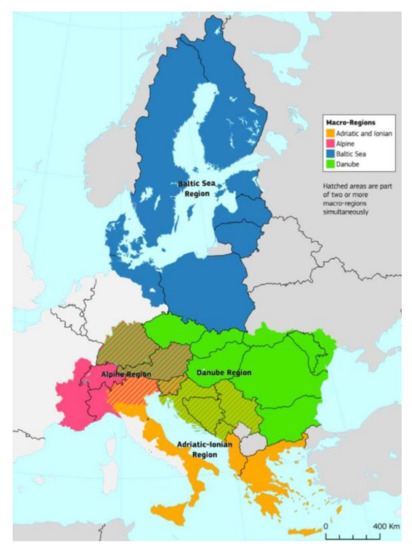
Figure 1.
EU macro-regions map (source: Ref. [43]).
The macro-regions’ strategies are each time accompanied by an Action Plan document. The Action Plan is one of the outputs of the Strategy approach. It aims to go from ‘words to actions’ by identifying the concrete priorities for a macro-region. Once an action or project is selected, it should be implemented by the countries and stakeholders concerned. The Action Plan structure is usually as follows:
- pillars;
- topics under each pillar;
- actions;
- projects (sometimes flagships that are joint transnational projects and processes that serve as a pilot example for a desired change).
While establishing actions and projects for macro-regions, the following criteria should be taken into account [44]:
- addressing identified priorities meeting well-substantiated needs;
- scope or impact should be transnational if it is not macro-regional;
- actions and plans should be realistic and credible;
- actions and plans should be built on existing initiatives;
- actions and plans should pay attention to the cross-cutting aspects;
- actions and plans should be coherent and mutually supportive.
3.1. Action Plan for Adriatic Ionian Region (EUSAIR)
From the point of view of this article, the focus should be at first paid to the Adriatic Ionian Region and its strategy known as EUSAIR. It consists of four EU countries: the eastern part of Italy, Greece, Slovenia, and Croatia, and four non-EU countries: Albania, Bosnia and Herzegovina, Montenegro, and Serbia, also called the “candidate countries”. The region itself represents around 70 million inhabitants, making up almost 14% of the EU population. The region is a functional area primarily defined by the Adriatic and Ionian Seas basin. Covering a crucial terrestrial surface area, it treats the marine, coastal, and terrestrial areas as interconnected systems. With intensified movements of goods, services, and peoples owing to Croatia’s accession to the EU and with the prospect of EU accession for other countries in the region, port hinterlands play a prominent role. Attention to land–sea linkages also highlights the impacts of unsustainable land-based activities on coastal areas and marine ecosystems. In the Action Plan for EUSAIR, the European Commission has meticulously described the pillars, topics, and actions planned for this region (examples in Table 1).

Table 1.
Action plan for EUSAIR.
Examples of projects implemented under the pillar Connecting the region and topic Maritime transport include, e.g., Ref. [44]:
- sharing strategic functions and harmonizing ports processes through a common Intelligent Transport System (ITS);
- certification of the ports on safety, sustainability, and computerization, as well as traffic monitoring and management;
- implementation of a system ensuring that data providers need to submit information only once, and that the information submitted is available for use in all relevant reporting and notification systems;
- establishing the clean shipping index that could help monitor emission and improve air quality in port cities;
- capacity-building activities (training, education programs, standardization, and interoperability) improving the application of international legal requirements;
- introducing the Traffic Separation Schemes (TSS) to predict the congested areas;
- developing ports, optimizing port interfaces, infrastructures, and procedures;
- implementation of Information and Communication Technology (ICT) and intelligent infrastructure services (e.g., tracking and monitoring) to improve the efficiency, reliability, and safety/security of the port operations and the delivery system;
- supporting multimodal port connectivity through the development of Short-Sea Shipping and the improvement of road and railway connections;
- green upgrading of ships, port machinery, and port activities (e.g., cranes, power supply from shore, fuel switching to LNG, retrofitting, etc.).
3.2. Action Plan for Baltic Sea Region (EUSBSR)
The second region considered in this paper is the Baltic Sea Region, and its strategy is known as EUSBSR. This region was the first to implement the macro-regional strategy in Europe (2009). It consists of eight EU countries: Estonia, Denmark, Finland, the northern part of Germany, Latvia, Lithuania, Poland, and Sweden, and cooperates with non-EU countries, such as Norway, Russia, Belarus, and Iceland. The region itself represents around 80 million inhabitants, making up almost 16% of the EU population. The EUSBSR is implemented in concrete joint projects and processes. Projects and processes named flagships of the EUSBSR demonstrate well the strategy’s progress. However, no new funding or institutions have been founded to support the implementation of the strategy. Instead, the EUSBSR, as all macro-regional Strategies, is based on the practical and more coordinated use of existing funding sources, and the promotion of synergies and complementarities. In the Action Plan for EUSBSR, the pillars (objectives) and topics (sub-objectives) were planned (Table 2).
Table 2.
Action plan for EUSBSR.
What is essential in this macro-region is that the actions were planned not only for individual pillars but also to implement selected areas of the EUSBSR policy. EUSBSR chosen Policy Areas (PA) division and actions corresponding to them and referring to EUSBSR pillars are presented in Table 3.
Table 3.
Division of EUSBSR Policy Areas (PA) and corresponding actions.
Some of the flagship projects under the Connect the region pillar and PA Transport are listed below [46]:
- EMMA-Enhancing freight mobility and logistics by strengthening inland waterway and river-sea transport, total budget: 4.4 mln Euro, implementation dates: March 2016–February 2019;
- TENTacle-Capitalising on TEN-T core transport network corridors for prosperity, growth, and cohesion, total budget: 3.8 mln Euro, implementation dates: May 2016–April 2019;
- NSB CoRe-North Sea Baltic connector of regions, total budget: 3.3 mln Euro, implementation dates: May 2016–April 2019;
- ScandriaR 2Act-Sustainable & multimodal transport in the Scandinavian Adriatic Corridor, total budget: 3.6 mln Euro, implementation dates: May 2016–April 2019;
- COMBINE-Strengthening Combined Transport in the Baltic Sea Region, total budget: 3.4 mln Euro, implementation dates: January 2019–June 2021.
3.3. Common Objectives for Macro-Regions in EUSAIR & EUSBSR
One can see that a critical element merging two macro-regions is transportation, not only by including the same pillar in both strategies (Connecting the region) but also through multi-faceted development of maritime aspects, including marine governance and services, clearing water in the sea, caring of rich and healthy wildlife, as well as safe shipping, developing a marine environment, and making the most of sea regions as frontrunners in tourism. The similarity of the regions is also expressed in their geographical sea surroundings or the population living in the countries and the targets distinguished in the strategies under the development of transportation in the pillar Connecting the region. However, analyzing the objectives in detail, it can be seen that the EUSAIR focuses on setting specific indicators, the achievement of which guarantees the successful implementation of the strategy’s objectives. Meanwhile, in the EUSBSR, there are rather general lines of action striving to develop the macro-region transportation network (Table 4).
Table 4.
Targets by 2020 in pillar Connecting the region.
Nevertheless, the assumptions of both the strategies of the macro-regions seem to be partially consistent with the White Paper on Transport vision, although the emphasis of the macro-regions on the development of maritime transport, which is somewhat omitted in the White Paper, draws attention. To achieve the goal of “thirty percent of road freight over 300 km should shift to other modes such as rail or waterborne transport by 2030, and more than 50% by 2050, facilitated by efficient and green freight corridors (…)” [47], it is right to aim at more efficient use of rail, air, and maritime transport, mainly because these three branches are characterized by lower gas emission rates than road transport. The European Commission indicates that the primary goal for transport is supporting mobility while reaching the 60% emission reduction target [47]. Unfortunately, it does not specify how to do it, but it gives a tool to modify the European transport network, which results in its continuous development and, at the same time, connecting regions (the Trans-European Transportation Network (TEN-T)). The problem is the reduction of gas emissions. The key seems not to be in changing the mode of transport. Solutions should be sought in the available infrastructure, both in the infrastructure that already exists and the infrastructure in which production will not generate additional increased greenhouse gas emissions and costs charging the member states’ budget. In 2019, 28.7% of total EU-28 greenhouse gas emissions came from the transport sector. Even though international aviation was responsible for the most significant percentage increase in greenhouse gas emissions since 1990 (+101.5%) and was followed by international shipping (+42%), these two emit fewer greenhouse gases than road transport.
In 2017, road transport was responsible for almost 72% of the total greenhouse gas emissions from transport (Figure 2). Of these emissions, 44% were from passenger cars, 9% from light commercial vehicles, and 19% from heavy-duty vehicles [48].
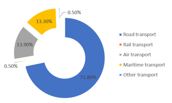
Figure 2.
Share of transport greenhouse gas emissions in 2017. Source: Ref. [48].
At the same time, the effect of the pandemic between 2020 and2021, which influenced the emission of gases from transport, cannot be ignored. According to scientists, the decrease in emissions was significant but not as large as estimated. According to a study [49], the most significant decrease in gas emissions was recorded in road transport, or, rather, land transport. Air transport was second in line. This was especially visible at the turn of March and April 2020, when most countries announced a simultaneous lockdown. Many airports have recorded significant drops in air traffic (in the summer season even at −33% in 2021 compared to 2019), which also translates into gas emissions.
Unfortunately, the change in total greenhouse gas emissions from transport between 1990 and 2017 in EU countries casts a shadow over the environmental performance of transport in general. Two of them with the best performance belong to the Baltic Sea Region (Sweden, Lithuania), but in the infamous tail of statistics lies Poland with almost the largest increase in gas emissions, by 206%, while the EU average is 28% (Figure 3).
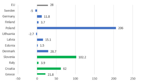
Figure 3.
Change in total greenhouse gas emissions from transport between 1990 and 2017 in % (blue—countries from EUSBSR; green—countries from EUSAIR). Source: Ref. [48].
In light of the presented statistics, it is hard not to doubt the possibility of achieving such divergent values of indicators as the 60% reduction in greenhouse gas emissions by 2050 suggested by the White Paper on Transport, while, in the last 30 years, in EU countries, gas emissions increased by an average of 30%. However, with this goal as the overarching one and, in addition to the targets set by macro-region strategies, one should look at the TEN-T network and the possibilities that this tool offers in terms of connecting regions taking into account environmental considerations.
4. Technical Aspects of Transportation in the EUSAIR & EUSBSR
Due to the information in Ref. [50], the main challenges for the transport sector in the EU include:
- creating a well-functioning Single European Transport Area,
- connecting Europe with modern, multimodal, and safe transport infrastructure networks,
- shifting towards low-emission mobility.
From a social perspective, affordability, reliability, and accessibility of transport are essential. Addressing these challenges will help pursue sustainable growth in the EU. That is why the Commission has started a couple of initiatives to develop the Single European Transport Area, such as:
- the 4th Railway Package;
- the Blue Belt initiatives for maritime transport;
- the proposed Single European Sky II;
- the EU Aviation Strategy;
- the NAIADES Programme for inland waterways.
In addition, to help EU countries develop the Trans-European Transport Network, the EU adopted a Regulation in 2013 providing guidelines for transport investment. The Regulation establishes a legally binding obligation for the EU countries to develop the so-called “Core” and “Comprehensive” TEN-T Networks and identifies projects of common interest and specifies the requirements to be complied with within the implementation of such projects. The TEN-T Core Network includes the most important connections, linking the most important nodes, while The TEN-T Comprehensive Network covers all European regions and will be completed by 2050. The Connecting Europe Facility (CEF) Regulation, adopted in 2013, allocated a seven-year budget (2014–2020) of EUR 30.4 billion, of which EUR 24 billion are for the transport sector [51]. On 2 May 2018, the Commission proposed a new long-term budget for the period of 2021 to 2027, where the focus remains on developing the Trans-European Network, with a particular priority on cross-border sections and missing links of the TEN-T Core Network.
4.1. Architecture of TEN-T
Nine TEN-T corridors pass through Europe. They connect the most critical transport points, such as seaports, airports, or transshipment points through rail, road, and inland waters networks. The corridors are as follows:
- Atlantic;
- Baltic–Adriatic;
- Mediterranean;
- North Sea–Baltic;
- North Sea–Mediterranean;
- Orient–East Mediterranean;
- Rhine–Alpine;
- Rhine–Danube;
- Scandinavian–Mediterranean.
Five of them: Baltic–Adriatic (dark blue), Mediterranean (green), Orient–East Mediterranean (brown), Rhine–Danube (light blue), and Scandinavian–Mediterranean (pink) pass through the Adriatic Ionian Region (Figure 4). Four of them: Baltic–Adriatic (dark blue), North Sea–Baltic (red), Orient–East Mediterranean (brown), and Scandinavian–Mediterranean (pink) pass through the Baltic Sea Region (Figure 5).
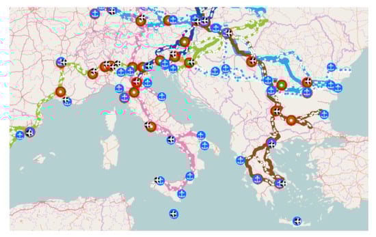
Figure 4.
TEN-T corridors in Adriatic Ionian Region. Source: Ref. [52].
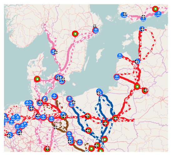
Figure 5.
TEN-T corridors in Baltic Sea Region. Source: Ref. [52].
The Baltic–Adriatic corridor has one of the most crucial road and railway axes in Central Europe. In this corridor, most funds are invested in rail transport. Moreover, in this branch, one can find the highest number of bottlenecks in project implementation. Road transport is the second most-subsidized mode of transport. Poland is mainly funded in this corridor [53].
The Mediterranean Corridor is the central east–west axis in the TEN-T Network. The corridor is 3000 km long and provides a multimodal link for ports of the Western Mediterranean with the center of the EU. It will let a modal shift from road to rail and connect some of the significant urban areas of the EU with high-speed trains. As in the previous corridor, most funds are also absorbed by rail transport, and this branch has the highest number of bottlenecks. The second branch in the order of subsidies is maritime transport. Among the macro-region countries analyzed, Italy receives the highest subsidy [54].
The North Sea–Baltic Corridor consists of 5947 km of railways, 4029 km of roads, and 2186 km of inland waterways and connects the ports of the eastern shore of the Baltic Sea with the ports of the North Sea. As in all of the six corridors passing through countries of the two analyzed macro-regions, in this one, rail is also funded chiefly. Similar to the Baltic–Adriatic Corridor, Poland achieved the highest amount of funds. Second, the most-funded branch is road transportation, especially intelligent transportation systems (ITS) [55].
The Orient–East Mediterranean Corridor connects the roads that pass through European countries in the north–south direction. The Work Plan of this corridor provides the implementation of 649 projects for EUR 89 billion. Rail transport accounts for the vast majority of the CEF fund. It is developed primarily in the southern part of the corridor (mainly Greece). In terms of investment, road transport is in second place. Here, it is worth paying attention to the fact that these are investments in motorways or express roads and alternative fuels (681 charging points are expected to be deployed) [56].
The Scandinavian–Mediterranean Corridor is interesting from the point of view of this article because it runs through the countries of both macro-regions and, at the same time, is the longest of all the TEN-T corridors. The CEF has granted 91 actions for a total investment worth EUR 6.4 billion. Once again, rail transport infrastructure receives the most funds (around EUR 2 billion). Maritime and road infrastructure will become greener because most actions focus on alternative fuel infrastructure [57].
The Rhine–Danube Corridor is interesting from the Croatian point of view. It links Central and South-Eastern Europe, but it passes only through Croatia from the macro-regional point. The Work Plan of this corridor includes, among all, a cross-border road bridge constructed between Croatia and Bosnia and Herzegovina on the Sava River. This can be treated as an example of successful cooperation because of the Rhine–Danube Core Network Corridor extension to the neighboring countries [58].
4.2. The Volume and Structure of Transport in EUSAIR & EUSBSR Countries
In order to summarize and understand investments in the area of transport in the TEN-T corridors, it is worth knowing the size and structure of transport in the countries of the macro-regions described. Rail transport will be analyzed first. Its importance in the development strategy of the macro-regions is exceptionally high. In the Work Plans of the individual TEN-T corridors, investments in rail transport are by far the largest. The question then arises: does the infrastructure and volume of rail transport in individual countries allow for the full use of this mode of transport? Firstly, in terms of infrastructure, rail transport is more developed in the Baltic Sea Region (EUSBSR). It is already visible in the analysis of the total length of railway lines in 2019 (Figure 6).
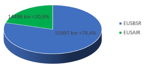
Figure 6.
The total length of railway lines in 2019 for macro-regions (where EUSBSR + EUSAIR = 100%). Source: (Total length of railway lines, https://ec.europa.eu/eurostat/databrowser/view/ttr00003/default/table?lang=en, accessed: 7 August 2021).
Secondly, the railway traffic is interesting, expressed by thousands of train kilometers. In the EUSBSR in 2019, this traffic was over three times higher than in EUSAIR. At the same time, even though Italy has a progressive movement individually, Germany is in the lead in the Baltic Sea Region, followed by Poland and then Sweden (Figure 7).
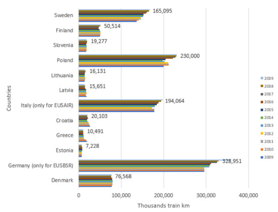
Figure 7.
Train movements in different countries in years 2009–2019. Source: (Train movements, https://ec.europa.eu/eurostat/databrowser/view/rail_tf_trainmv/default/table?lang=en, accessed: 7 August 2021).
The expenditures and individual investments of each country in railway infrastructure and rolling stock are also interesting. Although not all countries provide complete statistical information, the Baltic countries invest much more internal funds in rail transport than countries from the EUSAIR region. In case of investments in rolling stock, Poland invests the most prominent funds. It is a natural phenomenon related to the general development of rail transport in this country and rather the replacement of the several decades-old rolling stock with a new one and the implementation of high-speed railways, including the Pendolino. In turn, the largest expenditure on infrastructure was made in Sweden.
The situation is interesting in the case of maritime transport. Here, the assumptions of the EUSAIR Action Plan aimed at developing this particular mode of transport are not surprising. Maritime transport in both regions is characterized by handling of goods. Ultimately, the volume of the entire shipment in both macro-regions is comparable, and, in 2019, it accounted for 14.8% in the EUSBSR and 13.2% in the EUSAIR of all maritime transport in the EU countries (Figure 8).
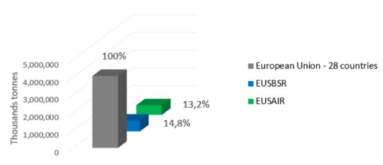
Figure 8.
The gross weight of goods handled in ports in EUSBSR & EUSAIR in comparison to EU in 2019. Source: (Gross weight of goods handled in all ports by direction-annual data, https://ec.europa.eu/eurostat/databrowser/view/mar_go_aa/default/table?lang=en, accessed: 7 August 2021).
As far as air transport is concerned, it should be emphasized that, despite the increase in gas emissions from this mode of transport in general, it still emits less of these gases together with maritime transport than the entire road transport. In the last decade, air transport recorded a significant increase in passengers handled. This was visible in Central Europe. For example, in Poland in 2011, more than 20 million passengers were handled, while, in 2019, there were more than twice as many, almost 47 million. The COVID-19 pandemic saw a dramatic drop to 14.5 million in 2020. The summary of the number of passengers handled in the countries of the macro-regions between 2017 and 2020 is presented in Figure 9.
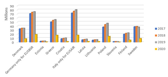
Figure 9.
Air passenger transport by reporting country in EUSBSR & EUSAIR 2017–2020. Source: (Air transport of passengers by country (yearly data), https://ec.europa.eu/eurostat/databrowser/view/ttr00012/default/table?lang=en, accessed: 22 August 2021).
Although Italy (even only for the EUSAIR region) is the leader in the carriage of passengers by air compared to other countries in 2019, the EUSBSR region countries carried more passengers in total. Germany was ranked second, followed by Greece. In total, however, as can be seen in Figure 10, passenger transport in the EUSBSR accounted for 21% of the total air transport in the EU, while, in the EUSAIR, it accounted for 13%.
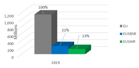
Figure 10.
Air passenger transport by regions EUSBSR & EUSAIR in 2019. Source: (Air transport of passengers by country (yearly data), https://ec.europa.eu/eurostat/databrowser/view/ttr00012/default/table?lang=en, accessed: 22 August 2021).
As for the infrastructure base, it is larger in the EUSBSR countries (Figure 11). However, this should be linked to the number of countries in this macro-region (8). In the EUSAIR region, the infrastructure is even more developed, but it is smaller due to the smaller number of countries (4) in total. Again, it is worth referring to the macro-region development strategy. In the EUSAIR, particular attention is paid to maritime transport. So far, however, due to the tourist nature of many areas of Italy or Greece, air transport has been the most preferred method of international transport.
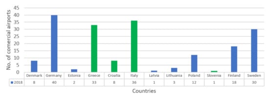
Figure 11.
Number of commercial airports in 2018 (blue—countries from EUSBSR; green—countries from EUSAIR). Source: (Number of commercial airports (with more than 15,000 passenger units per year), https://ec.europa.eu/eurostat/databrowser/view/avia_if_arp/default/table?lang=en, accessed: 22 August 2021).
Taking into account climate issues, mainly the fact that the level of gas emissions in maritime and aviation transport is similar (approximately 13% each), it is worth considering whether, instead of new investments in maritime infrastructure, it is better to use the current one, the existing aviation infrastructure, also in the field of freight transport and connecting the region in general.
As for road transport, to illustrate its size, in Figure 12, a comparison of the transport of goods (in thousands of tons) by various modes of transport in the countries of the macro-regions in 2019 is presented.
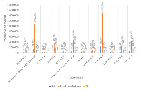
Figure 12.
Comparison of the transport of goods (in thousands of tons) by various modes of transport in the countries of the macro-regions in 2019. Source: (Goods transported, https://ec.europa.eu/eurostat/databrowser/view/rail_go_total/default/table?lang=en, accessed: 5 October 2021).
The last year before the coronavirus pandemic showed that the share of road transport in transporting goods was the highest in most macro-region countries. The exception was Estonia, where more goods were transported by sea. Some kind of diversification of transport can also be noticed in Latvia and Lithuania. However, road transport plays a key role. Of course, one can analyze the resources of road infrastructure, but, in light of the assumptions of the macro-region development strategies (EUSBSR & EUSAIR), it is necessary to consider which mode of transport in a given country and to what extent can replace the road one. For example, despite the well-developed infrastructure, the insignificant share of air transport is a wonder. Particularly noteworthy is rail transport, which has incurred enormous expenditure in recent years.
Moreover, the European Commission has declared 2021 the European Year of Rail as part of the EU’s efforts under the European Green Deal to achieve climate neutrality by 2050. In these modes of transport, there are also interesting cases of an increase in the share of the transport of goods during the pandemic (in 2020); i.e., Croatia recorded an increase in the transport of goods by rail in 2020 compared to previous years. In turn, Lithuania recorded such an increase in air transport.
4.3. Allocation of the CEF Funds
The Connecting Europe Facility (CEF) Regulation, adopted in 2013, allocated a seven-year budget (2014–2020) of EUR 30.4 billion, of which EUR 24 billion are for the transport sector [51]. On 2 May 2018, the Commission proposed a new long-term budget for the period of 2021 to 2027, where the focus remains on developing the Trans-European Network, with a particular priority on cross-border sections and missing links of the TEN-T Core Network. The allocation of CEF funds is a kind of exemplification of the actual needs and the direction of transport development. The division of the fund can be presented through the prism of the top five priority areas of planned investments and by type of transport. Below, in Table 5 and Table 6, the allocation of the fund (in millions of Euros) to the countries of the EUSBSR macro-region is shown. The lack of data in some table columns means that the budget was meager or no data were made available.
Table 5.
CEF transport top 5 priorities (mln Euro) in EUSBSR countries 2014–2020.
Table 6.
CEF transport per mode (mln Euro) in EUSBSR countries 2014–2020.
The largest allocation of CEF funds in the 2014–2020 financial perspective for the EUSBSR was recorded for the European Rail Traffic Management System. It is worth noting that almost 59% of these funds have been invested in Poland. The SESAR program turned out to be the second priority of CEF in terms of the amount of invested funds, with over 67% of them invested in Germany. Moreover, Poland’s participation in investments in the Intelligent Transport Services for road (ITS) program attracts attention. The analyzed financial perspective amounted to almost 98% of all funds spent on this priority.
The 2014 to 2020 CEF financial perspective for the EUSBSR can be characterized as a period of making high investments in rail transport with the share of almost 80% of CEF funds spent on all modes of transport. Considering over eight times greater expenditure on rail transport than on road transport and the aforementioned dominance of road transport in the context of the tonnage of transported goods, it requires reflection over the level of effectiveness of the implemented investments. Less than a 5% share of expenses on maritime transport also makes one think about the compliance of practical activities with the assumptions formulated in the EU Strategy for the Baltic Sea Region. Below, in Table 7 and Table 8, the allocation of the fund (in millions of Euros) to the countries of the EUSAIR macro-region is shown. As before, the amount of investment for five priority CEF programs and individual modes of transport has been presented in two separate tables.
Table 7.
CEF transport top 5 priorities (mln Euro) in EUSAIR countries 2014–2020.
Table 8.
CEF transport per mode (mln Euro) in EUSAIR countries 2014–2020.
The largest allocation of CEF funds in the 2014 to 2020 financial perspective for the EUSAIR was recorded for the Single European Sky-SESAR program. It is worth noting that almost 75% of these funds have been invested in Italy. ERTMS was next in terms of the size of investments. In this case, again, the most considerable amount of money was spent in Italy.
As in the case of the EUSBSR, also in the case of the EUSAIR, the analyzed financial perspective for 2014 to 2020 can be described as the period of major investments in rail transport. The issue of low expenses on maritime transport seems interesting again.
4.4. Correlation between the Size of the Investment and the Volume of Transport
An attempt was made to diagnose the linear relationships between the previously analyzed measures characterizing the scale of goods transport by various modes of transport based on CEF expenditure. For this purpose, the Pearson’s linear correlation coefficient was calculated using the formula below:
where:
- —ith values of observations from the population x;
- –ith values of observations from the population y.
For the analysis, the following factors were distinguished:
- —CEF expenditures on the rail;
- —CEF expenditures on European Rail Traffic Management System (ERTMS);
- —CEF expenditures on maritime;
- —CEF expenditure on Motorways of the Sea (MoS);
- —CEF expenditures on air transport;
- —CEF expenditures on Single European Sky ATM Research (SESAR);
- —CEF expenditures on road transport;
- —CEF expenditures on intelligent transportation systems (ITS);
- —CEF expenditures on new technologies;
- —transport of goods by rail in 2019 (in thousands of tons);
- —transport of goods by maritime in 2019 (in thousands of tons);
- —transport of goods by air transport in 2019 (in thousands of tons);
- —transport of goods by road transport in 2019 (in thousands of tons).
Values of these factors are presented in Appendix A.
Then, the Pearson’s linear correlation coefficient and the determination coefficient ( value in the relations presented in Table 9 were determined.
Table 9.
Pearson’s linear correlation coefficient and the determination coefficient for chosen relations.
Several interesting conclusions can be drawn from the presented statistical considerations:
- in the vast majority of observations, a strong or very strong correlation between the analyzed variables was diagnosed;
- the weakest correlation occurs in relation 4: the volume of goods transport in maritime transport has the lowest level of correlation with CEF expenditure on this mode of transport;
- at the same time, statistically, the volume of goods transport in maritime transport depends in 59% on the financial outlays made; the remaining 41% are other actions that should be taken to intensify the development of this transport. This conclusion is consistent with the EUSBSR and EUSAIR strategies, according to which macro-regions should take care of coastal tourism, sustainable development of fisheries, or ensuring the safety of shipping; see pillars: save the sea, blue growth. More effective activities in this area should increase the share of maritime transport in the transport of goods in the studied macro-regions.
4.5. Panel Data Model of Greenhouse Gas Emissions
Econometric analysis aimed to assess the significance and influence direction of the volume of freight transport (broken down by means of transport on the amount of air pollution with greenhouse gases. To compare EUSAIR to EUSBSR area in terms of transport impact on greenhouse gas emissions, two panel data models (NEUSAIR = 4, NEUSBSR = 8, T = 2005–2019) were constructed and estimated. A panel data regression differs from a regular time-series or cross-section regression in that it has a double subscript on its variables (2)
where i denotes the cross-section dimension, whereas t denotes the time-series [59] dimension, yit is a dependent variable, α is a scalar (constant term), β is K × 1, and xit is the i-th observation on K explanatory variables; denotes the error term.
From the point of view of econometric modeling, the most important feature is the possibility of avoiding bias of the estimator due to the omission of an important explanatory variable. It can lead to false, contradictory results. Models for panel data make it possible to estimate the individual effects of the factors impact (2), contributing to the differentiation of the observed units not included in the model, constant over time and/or (3) time effects, unchanged for all units, characteristic for individual years. There are two basic methods taking into account individual effects (individual or time). The fixed effect model (FEM) formulation assumes that differences across units (individuals or time) can be captured in the constant term. The fixed effect model takes (3) to be an unobservable, individual (or time)-specific constant term in the regression model [60].
The random effect model (REM) approach specifies that (4) is a group specific random element. The random effects model is appropriate for choosing N individuals randomly from a large population. In this case, N is usually large, and a fixed effects model would lead to an enormous loss of degrees of freedom.
where
denotes the unobservable individual (time)-specific effect and νit denotes the remainder disturbance.
Note that is time-invariant (or is individuals-invariant) and it accounts for any individual-specific effect (or time-specific effect) that is not included in the regression.
The following issue is estimating the indicated permanent effects (individual or time). The first model with intragroup effects, the so-called within model, uses deviations of a variable’s value from the group (individuals or time) average. The model is estimated without a constant using the Ordinary Last Squares (OLS). Estimated coefficients measure the effect of changes in the explanatory variable on the value of the dependent variable. The model does not take into account changes between groups. The second, between model, is computed on time (or individual) averages of the data, discards all the information due to intragroup variability but is consistent in some settings (e.g., nonstationarity) where the others are not, and is often preferred to estimate long-run relationships [59].
To choose the most appropriate estimator, the parameters and error terms hypotheses are tested using: (I) Testing for fixed effects (F-test). The null hypothesis is the same constant term applied across all individuals; (II) if the homogeneity assumption over the coefficients is established, the next step is to establish the presence of unobserved effects, comparing the null of spherical residuals with the alternative of individuals (or time units) specific effects in the error term (Breusch–Pagan test). (III) The choice between fixed and random effects specifications is based on Hausman test, comparing the two estimators under the null of no significant difference: if it is not rejected, the more efficient random effects estimator is chosen. In order to select the optimal model for inference, several models were estimated, taking into account the combinations of the above-mentioned methodological assumptions. The selection was then made based on the indicated statistical tests.
The first stage of constructing the theoretical form was selecting the functional form and indication of the dependent and explanatory variable. The dependent variable was assumed total national greenhouse gas emissions (from both ESD and ETS sectors) in tons per capita. This indicator included the so-called ‘Kyoto basket’ of greenhouse gases, that is, carbon dioxide (CO2), methane (CH4), nitrous oxide (N2O), and the so-called F-gases) from all sectors of the GHG emission inventories (including international aviation and indirect CO2) [61]. The explanatory variables were defined as the volumes of goods transported by road [62], rail [63], maritime [64], and air [65] transport in thousand tons. In order to take into account the economic importance of the transport modes, the volume of transported goods of each of them was divided by the GDP value of individual countries [66] (in Purchasing Power Standards, for EU-27, constant prices 2005 [67]). The power function was chosen as the functional form of the model. Estimates of explanatory variables parameters indicate the flexibility of changing the emission volume per capita to the change in the volume of loaded goods to GDP. After transforming the model equation into a linear form concerning the parameters (condition for the OLS estimator use), the theoretical model assumed the logarithmic form (5)
where:
denotes constant term,
, …, —estimated parameters,
—error term,
—total national greenhouse gas emissions in tons per capita in i-th country and t-th year;
—volumes of goods transported by road in thousand tons in terms of GDP i-th country and t-th year;
—volumes of goods transported by railway transport in thousand tons in terms of GDP i-th country and t-th year;
—gross weight of goods handled in all ports in thousand tons in terms of GDP i-th country and t-th year;
—volumes of freight and mail air transport in thousand tons in terms of GDP i-th country and t-th year.
One of the terms for using OLS is the lack of correlation between the explanatory variables. In order to verify this assumption, the Pearson linear correlation coefficients for the model variables were calculated (Table 10). It is necessary to point out a high relationship between the volume of cargo transported by rail and maritime transport (0.906). Despite the high correlation, it was decided to include the variable in the models. It is worth noting the occurrence of differences between EUSAIR and EUSBSR in the correlation of pollution and the tonnage of transported loads. In the group of EUSAIR countries, an increase in the tonnage of cargo transported by rail contributed only to reducing pollution. In the case of the EUSBSR countries, all types of transport, except air transport, showed such a relationship. Moreover, the correlations between the sizes of loads broken down by modes of transport indicate complementarity (maritime transport with road transport) and substitutability (air transport vs. road and railway transports).
Table 10.
Pearson’s linear correlation coefficients for EUSAIR and EUSBSR countries 2005–2019.
The next stage of the analysis was to estimate five variants panel data model: Pool (OLS), FEM (within-time), FEM (within-individual), FEM (between-time), REM (time). Before interpreting the results, the model with the best statistical properties was selected based on the tests (F-test, Breusch–Pagan test, Hausman test) (Table 11). The estimation results are presented in Table 12 and Table 13. Due to the comparability of the model estimation methods for the EUSAIR and EUSBSR, and high level of matching the models to empirical data (Adjusted R2), the Fixed Effect between the model for time units (FEM between-time) was selected. Interpretation of individual parameter estimation took into account the ceteris paribus assumption.
Table 11.
Results of panel data model tests.
Table 12.
Results of panel data models estimation for EUSAIR countries 2005–2019.
Table 13.
Results of panel data models estimation for EUSBSR countries 2005–2019.
The FEM (between-time) model estimation results (Table 12 and Table 13) show the following conclusions. Among the countries of both areas (EUSAIR, EUSBSR), the estimates showed a statistically significant (p < 0.05) positive impact on the volume of loads transported by road transport. An increase in volume loads by 1% resulted in an increase in air pollution by 0.446% (EUSAIR) and 0.728% (EUSBSR). In reference to loads’ road transport changes, the elasticity of air pollution was the highest compared to other modes of transport in the studied areas. This proves the highest emissivity of road transport.
5. Conclusions
The awareness of the role that transport plays in climate change makes it necessary to think about determining the directions that its individual modes should follow. In this context, it seems extremely important to look critically at international institutions’ strategies and action plans and integration groups associating individual countries and regions.
The article provides an in-depth review of the strategic documents of the Baltic Sea Region and Adriatic and Ionian Region in terms of their compliance with other EU strategic documents related to transport. An analysis and evaluation of official statistical data on the emissivity of individual modes of transport, the volume of transported goods, and the amount of expenditure incurred were performed. The main conclusions of the research carried out include:
- connecting the region is one of the main pillars of the strategic documents of the two analyzed EU macro-regions;
- the assumptions of both strategies of the macro-regions seem to be partially consistent with the White Paper on Transport vision, although the emphasis of macro-regions on the development of maritime transport, which is somewhat omitted in the White Paper, draws attention;
- the European Commission indicates that the primary goal for transport is growing transport and supporting mobility while reaching the 60% emission reduction target. Unfortunately, it does not specify how to achieve this;
- in light of the presented statistics, it is hard not to doubt the possibility of achieving such divergent values of indicators as the 60% reduction in greenhouse gas emissions by 2050, while, in the last 30 years, in EU countries, gas emissions increased by an average of 30%;
- the 2014–2020 CEF financial perspective for the EUSBSR and EUSAIR can be characterized as a period of making high investments in rail transport;
- considering over eight times greater expenditure on rail transport than on road transport in EUSBSR and over fifteen times greater in EUSAIR and the dominance of road transport in the context of the tonnage of transported goods, it requires reflection on the level of effectiveness of implemented investments;
- the volume of goods transport in maritime transport depends 59% on the financial outlays made; the remaining 41% are other actions that should be taken to intensify the development of this transport. Macro-regions should take care of the development of coastal tourism, sustainable development of fisheries, or ensuring shipping safety. More effective activities in this area should lead to an increase in the share of maritime transport in the transport of goods in the studied macro-regions;
- in the EUSAIR countries, an increase by 1% in the volume transport by railway resulted in a decrease in air pollution of greenhouse gases by 0.063%. Only in the case of the EUSAIR countries was this relationship significant (p < 0.05). In the case of the EUSAIR area containing the island countries, an increase in the volume of loads by 1% resulted in an increase in air pollution by 0.318%;
- in the EUSBSR countries, the elasticity of pollution growth to the size of air cargo amounted to −0.169%. In both analyzed areas, the impact of maritime transport turned out to be statistically insignificant.
The conclusions resulting from the analysis carried out in comparison with the recommendations of the European Commission presented in the White Paper Roadmap to a Single European Transport Area—Towards a competitive and resource efficient transport system indicate the following [47]:
- in point 24, the White Paper EC suggests that “Freight shipments over short and medium distances (below some 300 km) will to a considerable extent remain on trucks”—this is quite a controversial recommendation and seems to be correct only if the trucks are energy efficient, e.g., electric;
- point 26 of the White Paper coincides with the investments that were made (the largest ones for rail transport from the CEF fund); unfortunately, the level of use of railways by 2019 for the transport of goods does not indicate a significant increase compared to previous years, although there is a significant correlation between these factors;
- point 27 of the White Paper referring to seaports is consistent with the strategies of macro-regions, while the topic of inland waterways, for which limited funds in the CEF fund has been allocated, was rather cursory;
- point 29 of the White Paper refers to the proper use of maritime transport as a leader in long-haul transport, but the wording: “overall, the EU CO2 emissions from maritime transport should be cut by 40% (if feasible 50%) by 2050 compared to 2005 levels” deserves a reflection; the European Environment Agency in 2019 [48] reported that, firstly, over the last 20 years, CO2 emissions from maritime transport have already increased by 32%, and, secondly, that this emission will continue to increase (similar to air transport) and, until 2050, will increase by another 50 to 250% compared to 1990; at the same time, the European Parliament wants to take actions to make the maritime sector cleaner and more efficient in the transition to a climate-neutral Europe under the European Green Deal, e.g., phasing out heavy diesel fuels with compensation in the form of tax exemptions on alternative fuels or regulating access to EU ports for the most polluting ships, and technical improvements, such as vessel speed optimization, hydrodynamic innovation, new propulsion systems.
Considering the analyzed documentation, reports, strategies, and assumptions, it seems important to emphasize the role of rail transport in the decarbonization of transport. According to the authors, this branch of transport can significantly reduce the emission of gases into the atmosphere and thus contribute to the so-called “green deal”. However, many activities must be undertaken for this to happen, not only the investment ones. First of all, it is worth paying attention to the coherence of the regional strategies with the European transport development plan contained in the White Paper. Unfortunately, macro-regional strategies have a limited focus on rail transport and its role in the “connecting the region” pillar.
Author Contributions
Conceptualization, K.K.-P., M.P. and A.O.-K.; methodology, K.K.-P., M.P. and E.K.; validation, K.K.-P. and M.P.; formal analysis, K.K.-P., M.P., E.K. and A.O.-K.; investigation, K.K.-P., M.P. and A.O.-K.; resources, K.K.-P. and M.P.; data curation, K.K.-P. and M.P.; writing—original draft preparation, K.K.-P., M.P. and A.O.-K.; writing—review and editing, K.K.-P., M.P. and E.K.; visualization, K.K.-P.; funding acquisition, K.K.-P., M.P. and A.O.-K. All authors have read and agreed to the published version of the manuscript.
Funding
This research was partially funded by the Centre for Priority Research Area Artificial Intelligence and Robotics of Warsaw University of Technology within the Excellence Initiative: Research University (IDUB) Programme (Contract No. 1820/29/Z01/POB2/2021).
Institutional Review Board Statement
Not applicable.
Informed Consent Statement
Not applicable.
Data Availability Statement
The data presented in this study are openly available at https://ec.europa.eu/eurostat (accessed on 16 February 2022).
Conflicts of Interest
The authors declare no conflict of interest.
Appendix A
Table A1.
Values of observations from the population x and y.
Table A1.
Values of observations from the population x and y.
| Country | |||||||||||||
|---|---|---|---|---|---|---|---|---|---|---|---|---|---|
| Croatia | 266.1 | 0 | 98.1 | 0 | 25.8 | 25.8 | 28.7 | 13.5 | 6.9 | 14,449 | 20,580 | 11 | 81,125 |
| Greece | 509.9 | 0 | 31.9 | 31.3 | 22.5 | 22.5 | 7 | 0 | 7.4 | 1094 | 194,468 | 105 | 354,081 |
| Italy | 1193.4 | 103.1 | 106.8 | 0 | 143.7 | 143.7 | 73.5 | 41.2 | 56.6 | 47,148 | 254,037 | 511 | 489,442 |
| Slovenia | 278.2 | 6.4 | 11.3 | 0 | 4.5 | 0 | 37.1 | 8.8 | 15.5 | 21,902 | 22,114 | 11 | 91,775 |
| EUSAIR | 2247.6 | 109.5 | 248.1 | 31.3 | 196.5 | 192 | 146.3 | 63.5 | 86.4 | 84,593 | 491,199 | 638 | 1,016,423 |
| Estonia | 189 | 0 | 23.1 | 17.7 | 3.2 | 3.2 | 5.2 | 1.9 | 8.7 | 21,341 | 37,760 | 11 | 28,373 |
| Denmark | 719.5 | 12.8 | 23.3 | 21.8 | 32.5 | 32.5 | 49.2 | 0 | 45.1 | 8512 | 93,727 | 245 | 167,747 |
| Finland | 17.7 | 0 | 109.4 | 88.4 | 16.5 | 16.5 | 14.9 | 0 | 10.7 | 38,464 | 120,488 | 225 | 270,462 |
| Germany | 1765 | 103.4 | 23.2 | 0 | 261.7 | 261.2 | 158.1 | 0 | 105.3 | 121,373 | 98,178 | 1562 | 1,069,411 |
| Latvia | 259 | 1.1 | 0.9 | 0 | 2.6 | 2.6 | 9.4 | 1.1 | 8.3 | 41,490 | 59,046 | 26 | 73,755 |
| Lithuania | 342.9 | 0 | 13.2 | 13.2 | 9.6 | 9.6 | 23.4 | 0 | 0 | 55,209 | 52,244 | 17 | 100,802 |
| Poland | 3505.5 | 293 | 147.8 | 0 | 13.1 | 0 | 510.1 | 123 | 0 | 233,744 | 93,864 | 143 | 1,506,450 |
| Sweden | 152.5 | 88.9 | 73.5 | 60 | 63.3 | 63.6 | 46.1 | 0 | 36.6 | 72,896 | 170,557 | 148 | 449,362 |
| EUSBSR | 6951.1 | 499.2 | 414.4 | 201.1 | 402.5 | 389.2 | 816.4 | 126 | 214.7 | 593,029 | 725,864 | 2377 | 3,666,362 |
Source: own study.
References
- European Commission. A European Strategy for Low-Emission Mobility {COM(2016) 501 Final}; European Commission: Brussels, Belgium, 2016. [Google Scholar]
- Gløersen, E.; Balsiger, J.; Cugusi, B.; Debarbieux, B. The role of environmental issues in the adoption processes of European Union macro-regional strategies. Environ. Sci. Policy 2019, 97, 58–66. [Google Scholar] [CrossRef]
- Liu, Y.; Yuan, Y.; Guan, H.; Sun, X.; Huang, C. Technology and threshold: An empirical study of road passenger transport emissions. Res. Transp. Bus. Manag. 2021, 38, 100487. [Google Scholar] [CrossRef]
- Pita, P.; Winyuchakrit, P.; Limmeechokchai, B. Analysis of factors affecting energy consumption and CO2 emissions in Thailand’s road passenger transport. Heliyon 2020, 6, e05112. [Google Scholar] [CrossRef] [PubMed]
- Albayati, N.; Waisi, B.; Al-Furaiji, M.; Kadhom, M.; Alalwan, H. Effect of COVID-19 on air quality and pollution in different countries. J. Transp. Health 2021, 21, 101061. [Google Scholar] [CrossRef] [PubMed]
- Kazancoglu, Y.; Ozbiltekin-Pala, M.; Ozkan-Ozen, Y.D. Prediction and evaluation of greenhouse gas emissions for sustainable road transport within Europe. Sustain. Cities Soc. 2021, 70, 102924. [Google Scholar] [CrossRef]
- Matthias, V.; Bieser, J.; Mocanu, T.; Pregger, T.; Quante, M.; Ramacher, M.O.; Seum, S.; Winkler, C. Modelling road transport emissions in Germany—Current day situation and scenarios for 2040. Transp. Res. D Transp. Environ. 2020, 87, 102536. [Google Scholar] [CrossRef]
- Phillips, B.B.; Bullock, J.M.; Osborne, J.L.; Gaston, K.J. Spatial extent of road pollution: A national analysis. Sci. Total Environ. 2021, 773, 145589. [Google Scholar] [CrossRef]
- Calderon-Tellez, J.A.; Herrera, M.M. Appraising the impact of air transport on the environment: Lessons from the COVID-19 pandemic. Transp. Res. Interdiscip. Perspect. 2021, 10, 100351. [Google Scholar] [CrossRef]
- D’Alfonso, T.; Jiang, C.; Bracaglia, V. Would competition between air transport and high-speed rail benefit environment and social welfare? Transp. Res. B Methodol. 2015, 74, 118–137. [Google Scholar] [CrossRef]
- Zhang, F.; Wang, F.; Yao, S. High-speed rail accessibility and haze pollution in China: A spatial econometrics perspective. Transp. Res. D Transp. Environ. 2021, 94, 102802. [Google Scholar] [CrossRef]
- Guo, X.; Sun, W.; Yao, S.; Zheng, S. Does high-speed railway reduce air pollution along highways?—Evidence from China. Transp. Res. D Transp. Environ. 2020, 89, 102607. [Google Scholar] [CrossRef]
- Li, L.; Zhang, X. Reducing CO2 emissions through pricing, planning, and subsidizing rail freight. Transp. Res. D Transp. Environ. 2020, 87, 102483. [Google Scholar] [CrossRef]
- Lalive, R.; Luechinger, S.; Schmutzler, A. Does expanding regional train service reduce air pollution? J. Environ. Econ. Manag. 2018, 92, 744–764. [Google Scholar] [CrossRef]
- Cardenete, M.; López-Cabaco, R. Economic and environmental impact of the new Mediterranean Rail Corridor in Andalusia: A dynamic CGE approach. Transp. Policy 2021, 102, 25–34. [Google Scholar] [CrossRef]
- Troch, F.; Meersman, H.; Sys, C.; Van De Voorde, E.; Vanelslander, T. The added value of rail freight transport in Belgium. Res. Transp. Bus. Manag. 2021, 100625. [Google Scholar] [CrossRef]
- Georgakaki, A.; Coffey, R.A.; Lock, G.; Sorenson, S.C. Transport and Environment Database System (TRENDS): Maritime air pollutant emission modelling. Atmos. Environ. 2005, 39, 2357–2365. [Google Scholar] [CrossRef]
- Bagoulla, C.; Guillotreau, P. Maritime transport in the French economy and its impact on air pollution: An input-output analysis. Mar. Policy 2020, 116, 103818. [Google Scholar] [CrossRef]
- Wang, H.; Liu, D.; Dai, G. Review of maritime transportation air emission pollution and policy analysis. J. Ocean Univ. China 2009, 8, 283–290. [Google Scholar] [CrossRef]
- Nengye, L.; Maes, F. The European Union and the International Maritime Organization: EU’s external influence on the prevention of vessel-source pollution. J. Mar. L. Com. 2010, 41, 581. [Google Scholar]
- Taghvaee, S.M.; Omaraee, B.; Taghvaee, V.M. Maritime Transportation, Environmental Pollution, and Economic Growth in Iran: Using Dynamic Log Linear Model and Granger Causality Approach. Iran. Econ. Rev. 2017, 21, 185–210. [Google Scholar] [CrossRef]
- Al Fartoosi, F.M. The impact of maritime oil pollution in the marine environment: Case study of maritime oil pollution in the navigational channel of Shatt Al-Arab. Master’s Thesis, World Maritime University, Malmo, Sweden, 2013. [Google Scholar]
- Heij, C.; Bijwaard, G.; Knapp, S. Ship inspection strategies: Effects on maritime safety and environmental protection. Transp. Res. D Transp. Environ. 2011, 16, 42–48. [Google Scholar] [CrossRef]
- Lu, C.-S.; Liu, W.-H.; Wooldridge, C. Maritime environmental governance and green shipping. Marit. Policy Manag. 2014, 41, 131–133. [Google Scholar] [CrossRef]
- Lai, K.-H.; Lun, Y.H.; Wong, C.W.; Cheng, E. Green shipping practices in the shipping industry: Conceptualization, adoption, and implications. Resour. Conserv. Recycl. 2011, 55, 631–638. [Google Scholar] [CrossRef]
- Wan, Z.; Zhu, M.; Chen, S.; Sperling, D. Pollution: Three steps to a green shipping industry. Nature 2016, 530, 451–466. [Google Scholar] [CrossRef] [PubMed]
- Prokopenko, O.; Miskiewicz, R. Perception of ‘Green Shipping’ in the contemporary conditions. Entrep. Sustain. Issues 2020, 8, 269–284. [Google Scholar] [CrossRef]
- Niavis, S.; Papatheochari, T.; Kyratsoulis, T.; Coccossis, H. Revealing the potential of maritime transport for ‘Blue Economy’ in the Adriatic-Ionian Region. Case Stud. Transp. Policy 2017, 5, 380–388. [Google Scholar] [CrossRef]
- Merico, E.; Gambaro, A.; Argiriou, A.; Alebic-Juretic, A.; Barbaro, E.; Cesari, D.; Chasapidis, L.; Dimopoulos, S.; Dinoi, A.; Donateo, A.; et al. Atmospheric impact of ship traffic in four Adriatic-Ionian port-cities: Comparison and harmonization of different approaches. Transp. Res. D Transp. Environ. 2017, 50, 431–445. [Google Scholar] [CrossRef]
- Lindholm, M.; Behrends, S. Challenges in urban freight transport planning—A review in the Baltic Sea Region. J. Transp. Geogr. 2012, 22, 129–136. [Google Scholar] [CrossRef]
- Manzhynski, S.; Siniak, N.; Źróbek-Różańska, A.; Źróbek, S. Sustainability performance in the Baltic Sea Region. Land Use Policy 2016, 57, 489–498. [Google Scholar] [CrossRef]
- Goldmann, K.; Wessel, J. TEN-T corridors—Stairway to heaven or highway to hell? Transp. Res. Part A Policy Pract. 2020, 137, 240–258. [Google Scholar] [CrossRef]
- Öberg, M.; Nilsson, K.L.; Johansson, C.M. Complementary governance for sustainable development in transport: The European TEN-T Core network corridors. Case Stud. Transp. Policy 2018, 6, 674–682. [Google Scholar] [CrossRef]
- Öberg, M.; Nilsson, K.L.; Johansson, C. Major transport corridors: The concept of sustainability in EU documents. Transp. Res. Procedia 2017, 25, 3694–3702. [Google Scholar] [CrossRef]
- Aparicio, Á. The changing decision-making narratives in 25 years of TEN-T policies. Transp. Res. Procedia 2017, 25, 3715–3724. [Google Scholar] [CrossRef]
- Gutiérrez, J.; Condeço-Melhorado, A.; López, E.; Monzón, A. Evaluating the European added value of TEN-T projects: A methodological proposal based on spatial spillovers, accessibility and GIS. J. Transp. Geogr. 2011, 19, 840–850. [Google Scholar] [CrossRef]
- Otsuka, N.; Günther, F.C.; Tosoni, I.; Braun, C. Developing trans-European railway corridors: Lessons from the Rhine-Alpine Corridor. Case Stud. Transp. Policy 2017, 5, 527–536. [Google Scholar] [CrossRef]
- Van Weenen, R.L.; Burgess, A.; Francke, J. Study on the Implementation of the TEN-T Regulation—The Netherlands Case. Transp. Res. Procedia 2016, 14, 484–493. [Google Scholar] [CrossRef][Green Version]
- Heich, H.-J.; Jantunen, J.; Negrenti, E. The assessment of environmental and safety impacts of the trans-European transport network (TEN-T). Sci. Total Environ. 1999, 235, 391–393. [Google Scholar] [CrossRef]
- Trnka, M.; Ondrejka, R.; Danišovič, P.; Pitoňák, M. Support of Intermodal Transport in TRITIA Area. Transp. Res. Procedia 2021, 53, 234–243. [Google Scholar] [CrossRef]
- Schwedes, O.; Riedel, V.; Dziekan, K. Project planning vs. strategic planning: Promoting a different perspective for sustainable transport policy in European R&D projects. Case Stud. Transp. Policy 2017, 5, 31–37. [Google Scholar] [CrossRef]
- Castellano, R.; Musella, G.; Punzo, G. Exploring changes in the employment structure and wage inequality in Western Europe using the unconditional quantile regression. Empirica 2019, 46, 249–304. [Google Scholar] [CrossRef]
- EU Macro-Regional Strategies, Council of Europe. Available online: https://pjp-eu.coe.int/en/web/cultural-routes-and-regional-development/eu-macro-regions (accessed on 16 January 2020).
- European Commission. Action Plan Concerning the European Union Strategy for the Adriatic and Ionian Region {COM(2014) 357 Final}; European Commission: Brussels, Belgium, 2014. [Google Scholar]
- European Commission. European Union Strategy for the Baltic Sea Region ACTION PLAN {COM(2009) 248}; European Commission: Brussels, Belgium, 2015. [Google Scholar]
- Interreg Baltic Sea Region, Flagships of the EU Strategy for the Baltic Sea Region (EUSBSR). 2019. Available online: https://www.balticsea-region-strategy.eu/ (accessed on 25 January 2022).
- European Commission, Directorate-General for Mobility and Transport. White Paper on Transport: Roadmap to a Single European Transport Area: Towards a Competitive and Resource Efficient Transport System; European Commission: Brussels, Belgium, 2011. [Google Scholar] [CrossRef]
- European Environment Agency. Greenhouse Gas Emissions from Transport in Europe. Available online: https://www.eea.europa.eu/data-and-maps/indicators/transport-emissions-of-greenhouse-gases/transport-emissions-of-greenhouse-gases-12 (accessed on 6 August 2021).
- Le Quéré, C.; Jackson, R.B.; Jones, M.W.; Smith, A.; Abernethy, S.; Andrew, R.M.; De-Gol, A.J.; Willis, D.R.; Shan, Y.; Canadell, J.G.; et al. Temporary reduction in daily global CO2 emissions during the COVID-19 forced confinement. Nat. Clim. Chang. 2020, 10, 647–653. [Google Scholar] [CrossRef]
- European Commission. Mobility and Transport. Transport in the European Union. Current Trends and Issues; European Commission: Brussels, Belgium, 2019. [Google Scholar]
- Regulation (EU) No 1316/2013 of the European Parliament and of the Council of 11 December 2013 establishing the Connecting Europe Facility amended by Regulation 2015/1017 on the European Fund for Strategic Investments. Off. J. Eur. Un. 2013, 348, 129–170.
- TENtec Interactive Map Viewer. Available online: https://ec.europa.eu/transport/infrastructure/tentec/tentec-portal/map/maps.html (accessed on 5 April 2020).
- European Commission. CEF Support to Baltic-Adriatic Corridor; European Commission: Brussels, Belgium, 2020. [Google Scholar]
- European Commission. CEF Support to Mediterranean Corridor; European Commission: Brussels, Belgium, 2020. [Google Scholar]
- European Commission. CEF Support to North Sea-Baltic Corridor; European Commission: Brussels, Belgium, 2020. [Google Scholar]
- European Commission. CEF Support to Orient East-Mediterranean Corridor; European Commission: Brussels, Belgium, 2020. [Google Scholar]
- European Commission. CEF Support to Scandinavian-Mediterranean Corridor; European Commission: Brussels, Belgium, 2020. [Google Scholar]
- European Commission. CEF Support to Rhine-Danube Corridor; European Commission: Brussels, Belgium, 2020. [Google Scholar]
- Croissant, Y.; Giovanni, M. Panel Data Econometrics in R: The plm Package. J. Stat. Softw. 2008, 27. Available online: https://www.jstatsoft.org/article/download/v027i02/254 (accessed on 12 February 2020).
- Greene, W.H. Econometric Analysis, 5th ed.; Prentice Hall: Hoboken, NJ, USA, 2003. [Google Scholar]
- Eurostat Data Browser: Greenhouse Gas Emissions by Source Sector (Source: European Environment Agency), Tones Per Capita. Available online: https://ec.europa.eu/eurostat/databrowser/view/SDG_13_10__custom_2072644/default/table?lang=en (accessed on 10 February 2022).
- Eurostat Data Browser: Summary of Annual Road Freight Transport by Type of Operation and Type of Transport (1000 t, Mio Tkm, Mio Veh-km)]. Available online: https://ec.europa.eu/eurostat/databrowser/view/ROAD_GO_TA_TOTT__custom_2071920/default/table?lang=en (accessed on 10 February 2022).
- Eurostat Data Browser: Goods Transported by Railway Transport. Available online: https://ec.europa.eu/eurostat/databrowser/view/RAIL_GO_TOTAL__custom_2071685/default/table?lang=en (accessed on 10 February 2022).
- Eurostat Data Browser: Gross Weight of Goods Handled in All Ports by Direction—Annual Data. Available online: https://ec.europa.eu/eurostat/databrowser/view/MAR_GO_AA__custom_2071579/default/table?lang=en (accessed on 10 February 2022).
- Eurostat Data Browser: Overview of the Freight and Mail Air Transport by Country and Airports. Available online: https://ec.europa.eu/eurostat/databrowser/view/AVIA_GOOC__custom_2072325/default/table?lang=en (accessed on 10 February 2022).
- Eurostat Data Browser: GDP and Main Components (Output, Expenditure and Income). Available online: https://ec.europa.eu/eurostat/databrowser/view/NAMA_10_GDP__custom_2072803/default/table?lang=en (accessed on 10 February 2022).
- Eurostat Data Browser: GDP and Main Components (Output, Expenditure and Income), Price Index (Implicit Deflator), 2005 = 100. Available online: https://ec.europa.eu/eurostat/databrowser/view/NAMA_10_GDP__custom_2072840/default/table?lang=en (accessed on 10 February 2022).


Publisher’s Note: MDPI stays neutral with regard to jurisdictional claims in published maps and institutional affiliations. |
© 2022 by the authors. Licensee MDPI, Basel, Switzerland. This article is an open access article distributed under the terms and conditions of the Creative Commons Attribution (CC BY) license (https://creativecommons.org/licenses/by/4.0/).