How Does New Infrastructure Investment Affect Economic Growth Quality? Empirical Evidence from China

Abstract

The current phase of the technological revolution and the accelerated rate of industrial change have encouraged the structural transformation of global infrastructure investment. This study aims to identify and evaluate the impact of new infrastructure investment on economic growth quality. This paper explains the theoretical mechanisms in terms of their effects on technological innovation, industrial structure, and productivity, using the three-dimensional analysis framework of economic growth conditions, process, and results. We then carry out an empirical examination based on provincial panel data for China from 2004 to 2019. The findings demonstrate that new infrastructure investment can significantly improve economic growth quality, and this conclusion still seems valid after conducting endogeneity treatments and robustness tests. Further mechanism evaluations indicate that new infrastructure investments contribute to boosting economic growth quality in terms of the condition, process, and results of economic growth by promoting technological innovation, improving industrial structure, and enhancing production efficiency. Moreover, the magnitude and mechanism of the positive effects differ depending on the heterogeneity of the region examined. In terms of the nonlinear change characteristics, the significant dual-threshold effect reveals that the marginal effects of new infrastructure investment on economic growth quality tend to be incremental under the threshold condition. This study provides a theoretical and factual basis for governments to enforce new infrastructure investments in the digital economy era, and it also has some value as a reference regarding the economic sustainability of developing countries.

1. Introduction

The role of infrastructure investment in economic growth has been a central concern for economists. Early studies argued that traditional infrastructure investments, such as those into transportation, could contribute significantly to economic growth [1,2,3]. At the macro level, infrastructure investment can contribute to economic growth directly as an input factor, and indirectly by increasing the total factor productivity (TFP) through its scale and network effects [4,5,6,7]. At the micro level, infrastructure investment can help improve enterprises’ technical efficiency by reducing their operating and inventory cost [8,9].

At present, the new generation of general-purpose technologies and their related industrial developments are giving rise to a new round of technological innovation and industrial change, profoundly changing the organization of various industries and reshaping the landscape of international competition. With the continuous integration, overlapping iteration, and profound applicability of new general-purpose technologies, infrastructure construction is giving rise to digital transformation. The traditional form of infrastructure investment is slowly shifting in a new direction. Typically, the term “new infrastructure investment” refers to several vital areas of information infrastructure investment, such as 5G, industrial internet, Internet of Things, artificial intelligence, cloud computing, blockchain, and big data; it also includes investment in innovative infrastructure to support scientific research, technology development, and product development, as well as the transition towards digitalization and intelligence of traditional infrastructure [10]. Under the dual pressures of the increasing uncertainty of global economic development and the structural imbalance of supply and demand in the post-COVID-19 era, new infrastructure investments must balance the policy objectives of stimulating effective demand in the short term and increasing adequate supply in the long term. It becomes necessary to stimulate investment vitality and innovation potential, and to promote consumption and industrial upgrading.

The contributions of this paper are mainly as follows. At the theoretical level, taking the conditions, processes and results of economic growth as the entry point, this paper explains how new infrastructure investment affects economic growth quality. To fill the gap, we propose the research hypothesis that new infrastructure investment elevates economic growth quality by enhancing innovation capacity, improving industrial structure, and increasing production efficiency, but this effect appears to be regionally heterogeneous and is characterized by nonlinear change. At the empirical level, based on provincial panel data for China from 2004 to 2019, we intend to provide new evidence regarding the effects of new infrastructure investment on economic growth quality, evaluating the mechanism from the three perspectives of the driver of innovation in economic growth, the structural transition in the economic growth process, and the enhancement of efficiency in economic growth. We also conduct a heterogeneity analysis from the perspective of the regional characteristics, and examine nonlinear change from the stage perspective. Since large developing countries’ economic development models and structures are highly isomorphic [11], the findings of this paper have meaningful implications related to the economic sustainability of other developing countries, and especially those with emerging economies.

The novelty of this paper is as follows: firstly, in terms of academic thinking, we incorporate infrastructure investment into the analytical framework of economic growth quality impact factors. The economic impact of new infrastructure investment has been focused on in the context of the structural transformation of infrastructure investment. The boosting effect of new infrastructure investment on economic growth quality is assessed from both theoretical and empirical perspectives. Secondly, in terms of quantitative research methodology, to effectively deal with possible endogeneity problems such as omitted variables and reverse causality, we select historical data that meets the requirements of relevance and exclusivity as instrumental variables and adopts the instrumental variables method combined with the two-stage least squares (2SLS) estimation. In such a way, we can more rigorously identify causality and achieve consistent estimation results. Finally, in terms of academic views, the boosting effect of new infrastructure investment on the economic growth quality is believed to be comprehensive and systematic. It is reflected in the fact that new infrastructure investment can boost the economic growth quality through technological innovation effect, industrial structure effect, and productivity effect from the conditions, processes, and results of economic growth altogether. Thus, we gain new insights into how new infrastructure investment affects economic growth quality.

The remainder of this paper is organized as follows: Section 2 introduces the literature review. Section 3 describes the theoretical framework and presents the research hypotheses. Section 4 introduces the identification methodology, including the econometric model, variables, and data. Section 5 highlights and discusses the results of the empirical study, which included benchmark regression, endogeneity tests, robustness tests, and extended analyses, focusing on influence mechanisms, regional heterogeneity, and nonlinear characteristics. The last section contains the conclusions and policy implications.

2. Literature Review

“New infrastructure” is an infrastructure system that facilitates digital transformations, intelligent upgrades, and integrated innovation services [12]. An information infrastructure based on the evolution of a new generation of information technology is an integral part of the new infrastructure [13]. The benefits brought about by information infrastructure are not only limited to information technology investment itself, but can also generate positive externalities in many fields.

Theoretical studies at the enterprise level have shown that the construction of information infrastructure is accompanied by positive knowledge spillover effects, promoting the unconscious and inactive diffusion and penetration of knowledge among enterprises and accelerating the dissemination and utilization of knowledge, and this externality can increase the motivation of enterprises to invest in informatization, thus accordingly raising the level of enterprise informatization [14]. This increase can reduce the production costs and sales price of products, stimulate consumer demand, and thus promote the expansion of production scale and output [15]. In addition to this, it can make production technology more scientific and rational, and the production management process more convenient and efficient, thus improving production efficiency [16].

Another strand of the literature focuses on the macro level. A number of theoretical and empirical studies have shown that information and communication technology (ICT) infrastructure, broadband infrastructure, internet usage, and Internet of Things play significant roles in promoting economic growth [17,18,19,20]. Various panel data regressions have revealed the positive relationship between ICT capital and GDP growth in developing, emerging, and developed countries [21]. However, studies on the productivity effect of ICT investment have not reached consistent conclusions. Since Solow (1987) showed that the impact of computers on productivity was not statistically significant [22], several empirical studies have validated the “productivity paradox”, which states that large-scale ICT investment is not effective in improving efficiency [23,24]. Nevertheless, as ICT continues to develop and its integration with industrial development deepens, the role of ICT investment in enhancing labor productivity and TFP is being confirmed by many empirical studies [25]. Moreover, some analyses refer to an innovation effect, reporting a statistically significant positive effect of IT infrastructure on innovation performance [26], and an “inverted U” relation between technology infrastructure investment and technological innovation [27]. Digital economic innovation results in changes in the industrial structure and helps productivity improvement and cost reduction in the production sector [28].

Along with the rapid development of machine learning technology, scholars have begun to pay attention to the effects of artificial intelligence (AI), a new type of information infrastructure, on economic growth, employment, and industrial structural transformation. AI has the techno-economic characteristics of pervasiveness, substitution, synergy, and creativeness, enabling it to contribute to TFP in all sectors of the national economy by increasing factor contribution, improving input–output efficiency, and accelerating knowledge creation, thus contributing to macroeconomic growth [29,30].

There are two main approaches to portraying AI in the existing theoretical work. The first approach considers AI as a factor-expanding technology, represented by capital-expanding technology [31] and labor-expanding technology [32]. The relative substitutability of AI in areas of labor and capital depends on the capital and labor substitution elasticity. The second approach considers AI as a technology that enables automated production, and is thus more likely to be used to substitute labor [33]. Empirical study has been conducted to show the long-term productivity-augmenting and labor-reducing effects of implementing automation technologies in manufacturing companies [34]. In fact, only a small portion of labor is replaced by AI via automated production, since AI can also be used as an auxiliary tool to improve labor production efficiency, increasing the demand for specific skill-based labor that cannot be easily automated [35]. Hence, the impact of AI on industry employment represents more of a structural change, and it does not necessarily reduce overall labor demand [36].

Furthermore, the growth of the AI industry and the new business models and patterns it generates will promote the transformation and upgrading of the industrial structure [37]. AI does not have the same application prospects in different industries. For example, in the labor-intensive and capital-intensive manufacturing industries, the function of AI is to reduce labor and achieve low-cost customization; in technology-led and market-changing industries, the role of AI is to improve R&D efficiency and accurately predict and respond to the market [38].

A literature review has revealed that most theoretical and empirical studies focus on the impacts of different types of new infrastructure on economic activities, specifying three dimensions: macroeconomic, meso-industrial, and micro-enterprise. These cover the areas of economic growth, economic efficiency, and technological innovation at the macro level, the two key themes of industry employment and industrial upgrading at the industrial level, and the degree of informatization, the production scale, and the production efficiency at the micro level.

However, this approach has some shortcomings: firstly, the existing research has paid less attention to the impact of infrastructure investment on economic growth quality; secondly, most of the studies on new infrastructure, such as AI, employ only theoretical analyses and realistic summaries, and some of the empirical works do not pay enough attention to the endogeneity issue and lack sufficient empirical test; lastly, the existing studies focus more on information infrastructure, and there is little literature that directly studies the economic impact of new infrastructure investment as a whole. Accordingly, it is difficult to clarify the role and effects of new infrastructure investment in the area of high-quality economic growth, due to the lack of specific theoretical analyses and a rigorous process of causal identification. This provides room for academic exploration. Research on the impact of new infrastructure investment on economic growth quality can help us develop a new understanding of this important relationship.

3. Theoretical Framework and Research Hypothesis

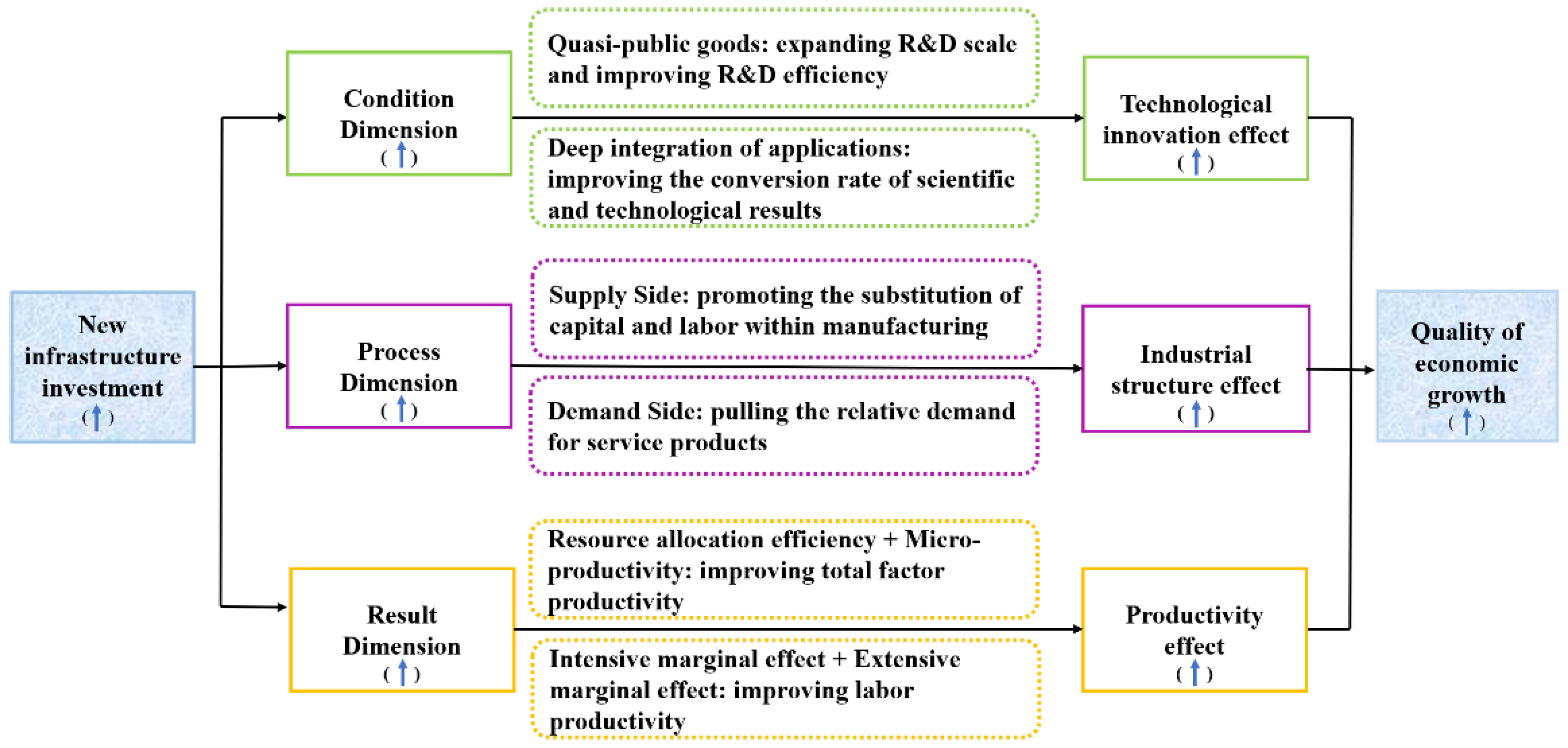
3.1. The Effect of New Infrastructure Investment on Economic Growth Quality

Economic growth refers to a unity of quantity and quality [39]. High-quality development refers to an advanced degree and optimal state of economic development. At the macroeconomic level, it relates to economic growth quality [40]. Early studies mainly considered economic growth quality when assessing the merits of economic growth, which can be addressed as the TFP in the context of economic growth efficiency [41]. Subsequent studies have taken a broader view of economic growth as covering different economic and social development aspects, incorporating issues such as income distribution, social welfare, resource consumption, and environmental pollution into the concept of growth quality [39,42]. The concept has been gradually enriched with the inclusion of process dimensions, such as structure, stability, and condition dimensions, including innovativeness and coordination [43,44,45]. Broadly speaking, the complex concept of economic growth quality involves normative value judgments about the condition, process, and results of economic growth. Therefore, in order to quantitatively expand economic growth to a particular stage, economic growth quality must be enhanced by improving the conditions, processes, and results at the same time.

New infrastructure represents an organic whole formed by the integrated application and linked operation of various new information technologies [10]. Traditional infrastructure such as transportation infrastructure can be defined as an underlying driver of many of the Sustainable Development Goals (SDGs) and a critical contributor that guarantees economic growth and socioeconomic benefits [46,47]. As new infrastructure involves supporting the transformation and upgrading of traditional infrastructure, the positive effect of new infrastructure on economic growth and regional sustainable development is consistent with transportation infrastructure [48]. With the demand for a digital economy and intelligent society, new infrastructure investment is essential for long-term sustainable development [10]. Compared with traditional infrastructure investment, new infrastructure investment has a more robust market orientation and higher economic and social benefits [13]. Comprehensively speaking, it has the characteristics of a high technology content and industry penetration rate, as well as substantial spillover and driving effects, generating a positive feedback mechanism with economic growth quality through its effects on technical innovation, industrial structure and productivity, in terms of the conditions, processes, and results of economic growth.

3.1.1. Economic Growth Condition: Technological Innovation Effect

Economic growth is reflected in the condition dimension as the essential ability to create national wealth by effectively exploiting various resources. High-quality economic growth requires the economic growth condition to be transformed from factor-driven to innovation-driven. New infrastructure investment stimulates innovation dynamics by expanding R&D scale, improving R&D efficiency, and promoting the conversion of scientific and technological innovation achievements.

On the one hand, technology infrastructure with quasi-public goods attributes formed by new infrastructure investment can effectively support the R&D of crucial core technologies, and provide guarantees of the innovation environment and innovation platform in order to strengthen the original innovation capacity and enhance the source supply of basic science [49]. This not only reduces R&D costs, improves R&D conditions, increases research equipment and knowledge-based human capital (thus contributing to the growth of R&D), but it also optimizes the allocation of R&D factors through positive externalities to enhance R&D efficiency, thus promoting the evolution of technological innovation from “technological imitation and integrated innovation” to “basic R&D and independent innovation”.

On the other hand, new infrastructure also refers to the infrastructure formed by applying new generation information technology to support the transformation and upgrading of economic and social infrastructure in the areas of transportation, energy, water conservation, education and medical care [10]. This provides plenty of application scenarios and grounds the broad market demand for intelligent and digital innovations conducive to improving the efficiency of scientific and technological achievements.

3.1.2. Economic Growth Process: Industrial Structure Effect

Economic growth manifests in the process dimension as the linkages and quantitative proportional relationships between elements within an economic system. High-quality economic development requires the economic growth process to allocate resources among industrial sectors rationally. New infrastructure investment promotes the substitution of capital-intensive industries for labor-intensive industries on the supply side, and boosts the demand of service industries relative to manufacturing industries on the demand side, which factors together empower the transformation and upgrading of industrial structure from both the supply and demand sides.

On the supply side, new infrastructure allows for autonomous manipulation, deep learning, the interconnection of everything, and human–machine interaction. These features give machines and equipment more powerful recognition, understanding, computation, and collaboration capabilities, making capital digital, intelligent and networked, as represented by capital-expanding technology that facilitates the substitution of capital for labor [31,33]. As a result, new infrastructure investment will significantly alter traditional production methods. This may substantially increase the marginal output of capital relative to labor, thus promoting the substitution of capital for labor within industries and increasing the output of capital-intensive industries, eventually enabling the transformation of industries from labor-intensive to capital-intensive and technology-intensive.

On the demand side, the construction and operation of new infrastructure requires R&D and the innovation of new information technologies in the relevant productive service industry [50]. For example, in terms of investment in the 5G industry, underlying technology R&D, the network operation service, the supply of core technology components, the information equipment manufacturing processes, and software application design are the main areas [51]; in investment in the artificial intelligence industry, automation, driverless operability, facial recognition, finance, education, and medical care are the main areas [38]. All of these rely on large investments in R&D and services. In short, new infrastructure investment represents a relatively higher share of production inputs in the service sector, contributing to higher employment and output in this sector by raising the relative demand for service sector products.

3.1.3. Economic Growth Result: Productivity Effect

Economic growth manifests in the result dimension as the effective conversion of various inputs into outputs and the sustainability of resources and the environment. High-quality economic growth refers to efficient and intensive growth. New infrastructure investments contribute to TFP growth by improving micro-production efficiency and resource-allocation efficiency, thus elevating labor productivity through intensive and extensive marginal effects, thereby enhancing economic growth efficiency.

The new generation of general-purpose technology facilitated by new infrastructure has the techno-economic characteristics of pervasiveness, substitution and synergy [52], all of which can enhance the fit between elements, reduce friction costs and improve production methods [53] via complementary investments in areas such as human capital and organizational management, the promotion of commercial model innovation, business procedure reshaping, and organizational structure changes, thus improving an enterprise’s micro-production efficiency. As the technological spillover effects of new infrastructures into other industries gradually unfold, industrial forms change, industrial boundaries become increasingly blurred, and industrial integration continues to deepen [12]. This disrupts the balance of resource allocation among and within industries, promoting the flow and transfer of production factors from industrial sectors with low productivity and low added value to those with high productivity and high added value, thereby improving resource allocation efficiency.

Consequently, new infrastructure investments improve the TFP of the entire industry, which directly enhances the labor productivity of each industrial sector; this manifests as the intensive marginal effect. This also indirectly affects the relative weights of industrial sectors with different degrees of labor productivity in the total labor productivity by promoting structural changes; this manifests as the extensive marginal effect [54].

3.2. Theoretical Hypothesis

Here, the effects of new infrastructure investment on economic growth quality can be deduced, as shown in Figure 1. Based on this deduction, this paper proposes the following theoretical hypotheses:

Hypothesis (H1).

New infrastructure investment contributes to the elevation of economic growth quality;

Hypothesis (H2).

New infrastructure investment elevates economic growth quality by enhancing innovation capacity, improving industrial structure, and increasing production efficiency.

Considering the different development bases, industrial supports, technology levels, undertaking capacities, and innovation capacities of each region, there are significant differences in the scale, operation effectiveness, and development potential of different kinds of new infrastructure investment [55]. A priori, the capital stock and investment efficiency of new infrastructure are distributed unevenly among regions. These objective regional differences may lead to differences in the effects of new infrastructure investment in various areas. In areas with greater economic strength, a stronger industrial base, high-quality enterprise clusters and business environments, abundant innovation resources and exhibiting technological advantages, the boosting effect of new infrastructure investment on economic growth quality can fully be utilized.

Furthermore, new infrastructure construction follows market rules and is influenced by macroeconomic policies; its role varies at different stages. In the initial phase, due to the small industry scale and the low completion and utilization rate, the effects of the technological innovation, industrial structure and productivity of new infrastructure investment will not have fully played out yet; thus, the degree of possible improvement in economic growth quality is limited. With the further expansion of the coverage and applicability of new infrastructures, the investment scale will continue to expand, and investment efficiency will steadily improve; its role in boosting economic growth quality thus gradually emerges. Neoclassical economic growth theory states that although infrastructure investment can promote economic growth and increase productivity, it is subject to the “law of diminishing marginal returns” due to the “crowding out effect” on private investment, as well as over-investment, the duplication of construction, and the waste of resources; as such, when there are limited resources, infrastructure investment is moderate [56]. In contrast, new infrastructure investment has the factor input characteristics of light materials and heavy technologies, and shows the characteristic trends of diminishing marginal costs and increasing marginal returns. With the continuous increase in new infrastructure investment, its marginal boosting effects on economic growth quality tend to strengthen.

Based on the above analysis, this paper proposes the following hypotheses:

Hypothesis (H3).

The impact of new infrastructure investments on economic growth quality appears to be regionally heterogeneous;

Hypothesis (H4).

The impact of new infrastructure investment on economic growth quality is characterized by nonlinear change.

4. Methodology and Data

4.1. Study Area

This paper chooses China as its subject because the transformation of China’s infrastructure investment has accelerated, driven by a series of policies [10]. The strength of traditional infrastructure investment (Traditional infrastructure investment is measured by the sum of fixed-asset investment in the “transportation, storage, and postal industry”, the “electricity, heat, gas and water production and supply industry”, and the “water, environment and public facilities management” industries.) has plummeted, with the growth rate dropping from about 15% per year in 2012–2017 to less than 5% per year in 2018–2019 [50]. New infrastructure investment is steadily rising, and has shown excellent growth potential. In 2019, the annual growth rate of fixed-asset investment in the internet and related service industries reached 16.7% [57]. New infrastructure investment in seven major areas (The seven areas include 5G base stations, ultra-high voltage, high-speed intercity railroads, urban rail transit, new energy vehicle charging piles, big data centers, artificial intelligence, and the industrial internet.) will reach CNY 10 trillion in 2025 [58]. It is worth noting that during previous high-speed economic growth phases, the expansion of traditional infrastructure investment made an enormous contribution to China’s rapid economic growth [4]. As economic growth slows down and shifts to a stage of high-quality development [59], can new infrastructure investment help improve the quality of China’s economic growth?

For such a purpose, this study has chosen 22 provinces, four autonomous regions, and four municipalities directly under the central government (excluding Taiwan and Tibet due to a lack of data), yielding a total of 30 provincial administrative regions as the research sample. China’s economic differentiation trends show regional imbalances between coastal and inland regions, given long-term influences such as geographic environment, economic policies, and factor endowments [60]. Based on the principle of combining economic development level and geographic location, the provinces were divided into three economic zones: eastern, central, and western regions [61]. To clearly show the geographical location of each sample province and the regional scope of each economic zone, the spatial distribution of eastern, central, and western regions is shown in Figure 2 using ArcGIS.

As shown in Figure 2, the eastern region contains 11 provinces that implemented the earliest coastal opening policies and which have become a center of growth that is driving the national economy. The central and western regions contain 20 inland provinces that maintain steady growth with the support of the regional development policy. In 2019, the eastern region accounted for about 11.1% of the national territory, 42% of the resident population, and 54% of the total GDP, and the per capita GDP here was higher than the national level. The central region accounted for about 17.5% of the national territory, 31% of the resident population, and 25% of the total GDP, while these ratios in the western region were 71.4%, 27%, and 21%, respectively. However, the GDP per capita in the central and western regions remains lower than the national level.

4.2. Econometric Methodology

Firstly, since the research sample in this paper is macro-level panel data, the fixed-effect model (FE) is chosen as the benchmark regression model to verify Hypothesis (H1) and identify the impact of new infrastructure investment on economic growth quality. The fixed-effect model has been widely used in panel data regression analysis [62]. As a general estimation strategy, it is assumed that individual regression equations have the same slope but can have different intercept terms [63]. Therefore, its advantage is that by introducing both individual heterogeneity and time heterogeneity into the model as dummy variables, the invisible individual differences and time differences are made visible [64]. Thus, the endogeneity of explanatory variables is eliminated to a certain extent and heterogeneity is better controlled. The benchmark regression model is set as follows:

$${\mathrm{grq}}_{it}={\alpha }_0+{\alpha }_1{\inf }_{it}+{{\displaystyle \sum }}_{p=1}^n{\theta }_p{X}_{it}+u_i+{\lambda }_t+{\epsilon }_{it}$$

(1)

where i stands for the province and t stands for the year; grq is the variable referring to economic growth quality; inf is the core explanatory variable referring to new infrastructure investment; $X_{it}$ is the set of control variables that include economic development level (gdp), urbanization level (urb), foreign investment dependence (fdi), transportation infrastructure level (tra), labor constraint (lab) and price level (pri); ${\epsilon }_{it}$ is the random error term; $u_i$ denotes province fixed effects. ${\lambda }_t$ is used to control time effects. If the coefficient ${\alpha }_1$ is positive and passes the significance test, this suggests that new infrastructure investment has the positive effect of promoting higher-quality economic growth.

Considering that the mean regression can only reflect the average marginal effect of new infrastructure investment on economic growth quality, this impact may differ under different conditional distributions. This article uses panel quantile regression to verify the impact of new infrastructure investment on economic growth quality at different quantile points to reflect a more comprehensive overview of the conditional distribution and exclude the influence of extreme values [65]. The specific model is set as follows:

$${\mathrm{grq}}_{it}=b_0+b_1\left(q\right){\inf }_{it}+{{\displaystyle \sum }}_{p=1}^n{\theta }_p{X}_{it}+u_i+{\lambda }_t+{\epsilon }_{it}$$

(2)

where the quantile points are divided into q = 0.25, 0.5, and 0.75, respectively.

Secondly, in testing Hypothesis (H2), we consider economic growth quality and three mediators as endogenous variables at the same time and construct the simultaneous equation model to verify the mediating effects of technological innovation, industrial structure and productivity. The underlying mechanisms behind relationships can be effectively explained by identifying mediating variables [66], which helps to understand how and why new infrastructure investment affect economic growth quality. Compared with the single equation, the structural equation can effectively identify the linkage between the disturbance terms of each equation and solve the endogeneity problem [67], so it is more suitable for testing the indirect transmission mechanism of new infrastructure investment on economic growth quality. The structural equation model is set as follows:

$$M_{it}=c_0+c_1{\inf }_{it}+{{\displaystyle \sum }}_{p=1}^n{\theta }_p{Z}_{it}+{\epsilon }_{it}$$

(3)

$${\mathrm{grq}}_{it}=d_0+d_1{M}_{it}+{{\displaystyle \sum }}_{p=1}^n{\theta }_p{X}_{it}+{\epsilon }_{it}$$

(4)

where $M_{it}$ represents the three mediators of technological innovation (tei), industrial structure (str), and productivity (ifp), respectively; the set of control variables $X_{it}$ is the same as those in Equation (1); the set of control variables $Z_{it}$ includes urbanization level (urb), foreign capital dependence (fdi), foreign trade dependence (dft), financial size (fin), human capital (huc), and government expenditure size (ges).

Thirdly, to test Hypothesis (H3) and determine the regional heterogeneity of the impact effect, the total sample is divided into two subsamples (inland region: Shanxi, Anhui, Jiangxi, Henan, Hubei, Hunan, Heilongjiang, Jilin, Inner Mongolia, Guangxi, Sichuan, Guizhou, Yunnan, Shaanxi, Gansu, Qinghai, Ningxia, Xinjiang. coastal region: Beijing, Tianjin, Hebei, Liaoning, Shanghai, Jiangsu, Zhejiang, Fujian, Shandong, Guangdong, and Hainan), comprising the inland and the coastal region. The econometric model is consistent with that shown in Equation (1).

Lastly, to test Hypothesis (H4) and analyze the nonlinear characteristics of the impact effect, drawing on Hansen (1999) [68], a panel threshold model is constructed by introducing new infrastructure investment (inf) as a threshold variable in the benchmark model:

$$\begin{array}{l}{\mathrm{grq}}_{it}={\pi }_0+{\pi }_1{\inf }_{it}\times I \left({\inf }_{it}\le {\phi }_1\right)+{\pi }_2{\inf }_{it}\times I\left({\phi }_1<{\inf }_{it}\le {\phi }_2\right)+\cdots +{\pi }_n{\inf }_{it}\times I({\phi }_{n-1}<{\inf }_{it}\le {\phi }_n)\\ \hspace{1em}\hspace{1em}\hspace{1em}\hspace{1em}\hspace{1em}\hspace{1em}\hspace{1em}+{\pi }_{n+1}{\inf }_{it}\times I\left({\inf }_{it}>{\phi }_n\right)+{{\displaystyle \sum }}_{p=1}^n{\theta }_p{X}_{it}+u_i+{\lambda }_t+{\epsilon }_{it}\end{array}$$

(5)

4.3. Variables Specification

4.3.1. Explained Variable: Economic Growth Quality (grq)

Economic growth has both quantitative and qualitative requirements [39]. The quantity of economic growth describes economic growth in terms of changes in the quantity of the entire economy, while the economic growth quality reflects economic growth in terms of its intrinsic nature [45]. Therefore, we believe that the economic growth quality refers to the intrinsic nature and law of economic growth, and the extent to which a series of inherent characteristics of economic growth meet the specific requirements of economic development. Specifically, it is the degree to which the material and service products that are grown by the economic activities meet the needs of the society to expand and reproduce and the needs of the people to continuously improve their lives. The judgment of the intrinsic nature and laws of economic growth should be examined in terms of not only its dynamic process, issue of consequences and prospects, but also its initial conditions. Thus, it requires discussion in three dimensions: condition, process, and result.

The economic growth quality is expressed in the condition dimension as the basic conditions and ability of an economy to effectively develop and utilize various resources to create wealth in the long term. High-quality economic growth is based on a high-quality national economy, which is centrally reflected in the accumulation of human and physical capital, the improvement of institutions, and the production, diffusion, and application of knowledge.

The economic growth quality is expressed in the process dimension as the structural changes caused by the changes in the linkage and proportional relations among the factors within the economic system. The structural changes in the economy bring about the flow of production factors from low-yielding to high-yielding sectors, and the resulting structural benefits provide a continuous impetus for high-quality economic growth. The optimization of industrial, consumption, and investment structure, and the increase in the scale of financial development and foreign trade during the process of economic growth can effectively adjust the economic structure and thus promote the transformation of economic growth.

The economic growth quality is expressed in the outcome dimension as the efficiency of transforming various inputs into outputs and the sustainability of resources and the environment. It is mainly related to the welfare changes and distribution of results of economic growth, as well as the cost of resource utilization and ecological environment. Good outcomes and prospects are the anchor point of high-quality economic growth. Furthermore, improving the efficiency of economic growth, reducing resource consumption and environmental pollution can significantly increase the net benefits of economic growth.

In summary, according to the above theoretical connotation of economic growth quality, the compound concept of economic growth quality is a comprehensive reflection of a series of factors. The measurement of economic growth quality needs to be measured and reflected by the comprehensive evaluation indexes composed of multiple aspects and indicators, which can measure and reflect the basic state of economic growth conditions, the fluctuation of the economic growth process, and the cost of economic growth results. Therefore, we have constructed a system of indicators for evaluating the economic growth quality, including 24 basic indicators, at the levels of the condition, process, and result of economic growth.

In the condition dimension of economic growth, to measure the basic conditions and capability level of national wealth creation, the basic indicators are selected from the perspective of factor endowment conditions and innovation capability. Factor endowment conditions involve the evaluation of human capital endowment, physical capital endowment, and institutional endowment level, while innovation capability involves the evaluation of innovation input level and innovation output level. Furthermore, the innovation input level includes the dimensions of R&D personnel input and capital input, and the innovation output level includes the dimensions of invention patent output and technology achievement output.

In the process dimension of economic growth, to measure the structure of economic growth, according to the System of National Accounts (SNA) and considering the typical dualistic economic structure of developing countries, the economic structure is divided into the industrial structure, investment-consumption structure, dualistic economic structure, financial structure, and balance of payments structure for measurement. More specifically, the industrial structure involves the evaluation of rationalization and advancement of the industrial structure. Investment and consumption structure involves the evaluation of both investment structure and consumption structure. The dual economy structure involves the evaluation of the allocation of output and labor between the agricultural and non-agricultural sectors. The financial structure involves the evaluation of the scale of financial development. The balance of payments structure involves the evaluation of the dependence on foreign trade.

In the outcome dimension of economic growth, to measure the input-output efficiency, welfare improvement, and resource and environmental cost of economic growth, the basic indicators are selected from growth efficiency, growth welfare and growth cost, respectively. Economic growth efficiency involves the evaluation of labor productivity, capital productivity, and total factor productivity. Economic growth welfare involves the evaluation from the aspects of health, income distribution, and employment. The cost of economic growth involves the evaluation of resource consumption and environmental pollution levels.

The entropy method is used to comprehensively assess economic growth quality. By calculating the entropy values and weights of all the indicators, the economic growth quality index is synthesized to quantify the economic growth quality. The indicators in each dimension are empowered with the same method to measure the condition index, process index, and result index. The evaluation system of economic growth quality is shown in

Table A1. Evaluation system of economic growth quality.

Dimension	Subindex	Basic Indicator	Proxy Variables	Attribute
Economic growth condition	Innovation capabilities	Innovation input	The ratio of expenditure on R&D to GDP.	+
			Full-time equivalent of R&D personnel.	+
		Innovation output	Number of invention patents granted.	+
			The ratio of technology market turnover to GDP.	+
	Element endowment	Human capital	Average years of education of schooling.	+
		Factor endowment structure	Capital stock per labor.	+
		Degree of marketization	Marketability index (the marketization index consists of five aspects: government–market relationship, the development of a non-state economy, the development of product markets, the development of factor markets, the development of market intermediary organizations, and the rule of law environment. The related data are derived from China Marketability Index Database).	+
Economic growth process	Industry structure	Rationalization of industrial structure	Thiel index of structural deviations (the formula for measuring industrial structure rationalization is $T{L}_{it}=\sum _{i=1}^n(\frac{Q_{it}}{Q_t})\ln [(\frac{Q_{it}}{L_{it}})/(\frac{Q_t}{L_t})]$, where TL denotes the Thiel index of structural deviation, and the smaller the value, the more rational the industrial structure. i denotes the industrial sector; n denotes the total number of industries; Q represents the industrial output; L represents the number of industrial employees).	-
		Advancement in industrial structure	Advanced index of industrial structure (the formula for measuring industrial structure advancement is $G{J}_{it}=\sum _{i=1}^n(Q_{it}/Q_t)\times \left(L{P}_{it}/L{P}_{if}\right)$, where GJ denotes the advanced index of industrial structure, and the higher the value, the more advanced the industrial structure. The meanings of i, n, and Q are the same as in Note 4; LP represents the labor productivity, and $L{P}_{if}$ represents the labor productivity at the completion of industrialization).	+
	Investment and consumption structure	Investment structure	The proportion of manufacturing fixed-asset investment in total fixed-asset investment	Moderate
		Consumption structure	The Engel coefficient of urban households	Moderate
	Dualistic economic structure	Dual comparative coefficient	The ratio of comparative labor productivity (comparative labor productivity is equal to the ratio of the share of industry output to the share of employment) in agriculture to comparative labor productivity in non-agricultural industries.	+
		Dual contrast index	Absolute value of the difference between the share of non-agricultural output and the share of employment.	-
	Financial development	Scale of financial development	The ratio of deposit and loan balances of financial institutions to GDP.	+
	Foreign trade	Foreign trade dependence	The ratio of gross imports and exports to GDP.	+
Economic growth result	Growth efficiency	Labor productivity	The ratio of GDP to the number of employees.	+
		Capital productivity	The ratio of GDP to capital stock.	+
		TFP	TFP growth rate.	+
	Growth benefit	Resident health	population mortality rate.	-
		Income distribution	The ratio of per capita disposable income of urban residents to per capita net income of rural residents.	-
		Employment opportunities	Urban registered unemployment rate.	-
	Growth cost	Resource consumption	Energy consumption per unit of GDP.	-
		Environmental pollution	Emissions of air pollutants per unit of output.	-
			Solid waste emissions per unit of output.	-

, and the calculation process of economic growth quality is shown in Appendix A.2.

The average values of the economic growth quality index and each dimension index of each province during the sampling period are shown in Figure 3. China’s economic growth quality shows significant regional characteristics. The provinces with higher economic growth quality are concentrated in the eastern region, with the Yangtze River Delta and the Pearl River Delta taking the lead, and more specifically with Beijing, Shanghai, Jiangsu, Guangdong, and Zhejiang at the forefront. Meanwhile, the economic growth quality in the central and western regions is generally lower, with a significant gap between it and the eastern coastal region; in particular, the shortcomings in economic growth quality are most pronounced in Yunnan, Gansu, Guizhou, Ningxia and Qinghai in the northwest.

4.3.2. Core Explanatory Variable: New Infrastructure Investment (Inf)

The level of new infrastructure investment is measured by the intensity of this investment, and the capital stock of new infrastructure is used for the robustness test. New infrastructure is divided into information infrastructure, convergence infrastructure and innovation infrastructure [69]. More specifically, information infrastructure includes communication network infrastructure, such as 5G, Internet of Things, the industrial internet, and satellite internet; new technology infrastructure such as artificial intelligence, cloud computing, and blockchain; arithmetic infrastructure such as data centers and intelligent computing centers. Convergence infrastructure mainly involves intelligent transportation and energy infrastructure. Innovation infrastructure involves major science and technology infrastructure, science and education infrastructure, and industrial technology innovation infrastructure.

Although the construction of new infrastructure is still in the embryonic stage, fixed-asset investments in the industry to which said infrastructure belongs represent the most established form of capital input [13]. Therefore, according to the sectors to which the various types of new infrastructure belong, the sum of urban fixed-asset investments in the internet and related services industry (the data on urban fixed-asset investment in the internet and related services industry by region, from 2004 to 2011, are not available in the official statistical yearbook. As such, the average proportion of urban fixed-asset investment in the internet and related services industry in each province from 2012 to 2019 is used as the allocation ratio, which is multiplied by the level of national urban fixed-asset investment in the internet and related services industry from 2004 to 2011 to estimate the provincial urban fixed-asset investment in the internet and related services industry from 2004 to 2011), the software and information technology services industry (China’s national industry classification standards were adjusted in 2012, and according to these, the pre-adjustment computer services and software industries are basically equivalent to the modified software and information technology service industry), and the scientific research and technology services industry is taken as the total new infrastructure investment. The intensity of new infrastructure investment equals the ratio of total new infrastructure investment to GDP. Based on this, the capital stock of new infrastructure is measured using the perpetual inventory method, in which the depreciation rate is 9% [70], and the fixed-asset price index (based on the 2003 level) is used to deflate the newly increased urban fixed-asset investment (The rate of fixed-asset delivery utilization in each industry is multiplied by the urban fixed-asset investment to estimate the newly increased urban fixed-asset investment).

4.3.3. Control Variables

Economic development level (gdp) is expressed by the logarithm of GDP per capita at a constant price, using 2003 as the base period.

Urbanization level (urb) is expressed by the proportion of the urban population within the total population.

Foreign investment dependency (fdi) is expressed by the proportion of foreign investment in the actual funds utilized for fixed-asset investment in the society as a whole.

Transportation infrastructure level (tra) is expressed by the logarithm of road mileage.

Labor constraint (lab) is expressed by the children and elderly dependency ratio in the population.

Foreign trade dependency (dft) is expressed by the ratio of gross imports and exports to GDP.

Financial scale (fin) is expressed by the ratio of the deposit and loan balances of the financial institutions to the GDP.

Human capital (huc) is expressed by the average years of schooling. Average years of schooling = the proportion of the population with elementary school education × 6 + the proportion of the population with junior high school education × 9 + the proportion of the population with senior high school education × 12 + the proportion of the population with a college education or above × 16.

Government expenditure scale (ges) is expressed by the ratio of fiscal expenditure to GDP.

4.3.4. Mediating Variables

Technological innovation (tei) is represented by the regional innovation capacity index, which is derived from the China Regional Innovation Capacity Monitoring Report. This measures regional innovation capacity in terms of innovation environment, innovation resources, enterprise innovation, innovation output, and innovation performance.

Industrial structure (str) is represented by the industrial structure hierarchy coefficient, calculated by the formula ${\mathrm{str}}_{it}=\sum _{i=1}^3{y}_{it}\times i$, where $y_i$ is the proportion of the industry output value to GDP. The larger the industrial structure hierarchy coefficient, the more optimized the industrial structure.

Productivity (ifp) is represented by the contribution of total factor productivity growth to economic growth, which is equal to the proportion of the total factor productivity growth rate to the economic growth rate. The total factor productivity growth rate is estimated via stochastic frontier analysis based on the transcendental logarithmic production function. The output is the real GDP, with 2003 taken as the base period. The labor input is the number of employees. Capital input is the capital stock estimated by the perpetual inventory method, in which the depreciation rate is 10.96%. Since the official data have not yet been published on the 2018–2019 gross capital formation by province, the regional total of social fixed-asset investment is used instead in order to calculate the capital stock for 2018–2019. The total factor productivity growth rate from 2004 to 2017 is re-measured by excluding the 2018–2019 data from the robustness test.

4.3.5. Data Sources and Description

The data adopted in this study refer to 30 provinces of China during the period 2004–2019, excluding Tibet, Hong Kong, Macao, and Taiwan, and Chongqing is examined together with Sichuan to maintain consistency and accuracy in the data. All data were collected from the China Statistical Yearbook, China Statistical Yearbook of Fixed Asset Investment, China Statistical Yearbook of Science and Technology, China Statistical Yearbook of Environment, China Financial Yearbook, China Statistical Yearbook of Cities, China Regional Innovation Capacity Monitoring Report, as well as provincial statistical yearbooks and the China Marketability Index Database. The descriptive statistics of the variables are shown in

Table 1. Descriptive statistics of variables.

Variables	Observations	Average Value	Standard Deviation	Minimum Value	Maximum Value
grq	464	0.0345	0.0040	0.0260	0.0469
inf	464	0.0071	0.0067	0.0005	0.0451
gdp	464	10.1161	0.6534	8.3158	11.6717
urb	464	0.5303	0.1476	0.1583	0.8960
fdi	464	0.0162	0.0215	0.0001	0.1518
tra	464	11.5055	0.9053	8.9625	13.2027
lab	464	0.3632	0.0694	0.1930	0.5760
pri	464	0.0274	0.0179	−0.0235	0.1009
dft	464	0.3579	0.4381	0.0020	2.0344
fin	464	1.2967	0.8540	0.5372	13.3605
huc	464	8.8330	1.0166	6.3778	12.6811
ges	464	0.2188	0.0984	0.0792	0.6284
tei	464	0.0345	0.0173	0.0076	0.1386
str	464	2.0035	0.2502	1.3878	2.7979
ifp	464	0.3046	0.1209	−0.8577	0.8477

.

5. Empirical Results and Discussion

5.1. Benchmark Estimated Results

The results of the Hausman test show that the fixed-effects model is better than the random-effects model. On this basis, the Wald test for between-group heteroscedasticity, the Wald test for within-group autocorrelation, and the Pesaran test for between-group contemporaneous correlation have been conducted within the fixed-effects model, and the test results show that the original hypotheses of “homoscedasticity, no first-order within-group autocorrelation, and no contemporaneous correlation” can be strongly rejected at the 1% level of significance. To effectively deal with the heteroscedasticity, serial correlation, and cross-sectional correlation problems, this paper uses a fixed-effect model (FE) together with the method proposed by Driscoll and Kraay (1998) to obtain the “heteroscedasticity–serial correlation–sectional correlation” robust standard error [71]. Since the feasible generalized least square (FGLS) can also be used to solve the heteroscedasticity, serial correlation, and cross-sectional correlation problems to a certain extent, the comprehensive FGLS has been used for estimation [72], and to avoid losing more degrees of freedom, the time trend term has been used instead of the time dummy variable to control for the time effect. The results of the benchmark regression are shown in

Table 2. Results of the benchmark regression.

Variables	Regression of Mean		Regression of Quantile
	FE	FGLS	25% Quantile	50% Quantile	75% Quantile
inf	0.0118 **	0.0108 ***	0.0193 ***	0.0209 ***	0.0279 ***
	(2.55)	(4.23)	(11.97)	(5.56)	(157.81)
gdp	0.0043 ***	0.0043 ***	0.0046 ***	0.0051 ***	0.0048 ***
	(11.26)	(25.37)	(31.04)	(172.12)	(881.87)
urb	0.0068 ***	0.0061 ***	0.0203 ***	0.0155 ***	0.0180 ***
	(6.49)	(6.74)	(39.84)	(112.28)	(387.57)
fdi	0.0072 ***	0.0061 ***	0.0019 ***	0.0121 ***	0.0143 ***
	(3.54)	(4.88)	(2.856)	(18.71)	(133.86)
tra	0.0006 ***	0.0005 ***	0.0019 ***	0.0013 ***	0.0005 ***
	(5.97)	(7.35)	(93.75)	(74.17)	(560.89)
lab	−0.0047 ***	−0.0027 ***	0.0134 ***	−0.0162 ***	−0.0208 ***
	(−2.84)	(−4.34)	(39.16)	(−35.23)	(−424.67)
pri	−0.0075	−0.0046 ***	−0.0364 ***	−0.0098 **	0.0077 ***
	(−1.18)	(−2.78)	(−21.43)	(−2.48)	(23.76)
cons	−0.0207 ***	−0.0196 ***
	(−5.26)	(−13.11)
Time Effects	Yes	Yes	Yes	Yes	Yes
Province Fixed Effect	Yes	Yes	Yes	Yes	Yes
F-Statistic	132.48 ***
Within-R2	0.3985
${\chi }^2$-Statistic		11,459.41 ***
Observations	464	464	464	464	464

Note **, ***, respectively, represent significance at the 10%, 5%, and 1% levels; the t value is shown in brackets for the FE regression, while the z value is shown in brackets for the FGLS and quantile regression.

.

The first column of Table 2 shows the estimation results of the two-way fixed-effect model. The estimated coefficient of new infrastructure investment is positive and passes the 5% significance test, controlling for the time and area fixed effect as well as the control variables. The economic growth quality index increases by 0.012% for every 1% increase in new infrastructure investment intensity, other things being equal. The FGLS estimation results in the second column of Table 2 show that the estimated coefficient of new infrastructure investment is 0.011, and is significant at the 1% level, which is slightly lower than the estimated coefficient of the fixed-effect model. The last three columns in Table 2 show the results of the panel quantile regression, where the estimated coefficients of new infrastructure investment are significantly positive at the 25%, 50%, and 75% quantile points. This positive impact tends to increase with increasing quartiles, indicating that new infrastructure investment plays a more significant role in regions with greater economic growth quality. Among the control variables, the coefficients of gdp, urb, fdi, and tra are shown to be significantly positive in the mean regression, the coefficient of pri is significantly negative, and the coefficient of lab is significantly negative under FGLS estimation, but is insignificantly so under FE estimation. This means that the increases in economic development level, urbanization level, foreign capital dependency, and transportation condition significantly contributed to economic growth quality. This conclusion is also consistent with the findings of existing relevant empirical studies [34,73]. On the contrary, the increases in price level and labor constraint have significant inhibitory effects on economic growth quality. In summary, the results of the benchmark regression verify Hypothesis (H1), which states that new infrastructure investment can significantly improve economic growth quality. It has been shown that infrastructure investment has a significant enhancing effect on the quality of economic growth [74], and the findings of the empirical study in this paper further point out that the boosting effect of new infrastructure investment on the quality of economic growth is also significant.

5.2. Endogeneity Problem and Treatment

Alleviating the endogeneity problem is an important issue in economics research that cannot be ignored. From the subject of concern in this paper, on one hand, the rapid improvement of economic growth quality cannot be separated from the rapid development of new infrastructure. At the same time, the development of new infrastructure cannot be separated from the improvement of economic growth quality, so there is a certain causal endogeneity between investment in new infrastructure and economic growth quality. On the other hand, there are many factors affecting economic growth quality, and the control variables involved in the current econometric model make it difficult to prevent the creation of omitted variables. Considering the possible reverse causality between new infrastructure investment and economic growth quality, as well as omitted variables, this paper adopts the instrumental variable method to mitigate endogeneity and identifies the causal effects of the impact of new infrastructure investment on economic growth quality. A reasonable instrumental variable needs to satisfy the relevance requirement and the exclusivity requirement. We choose the instrumental variables of new infrastructure investment on the basis of these two requirements.

On the one hand, from the perspective of the development history of new infrastructure, it has been developed based on the popularization of Internet technology. Meanwhile, from the perspective of the development history of Internet access technology, the Internet came into the public view from the telephone line dial-up access (PSTN), followed by ISDN, ADSL access to the current fiber-optic broadband access technology. Therefore, the development of Internet technology should start from the popularization of fixed-line telephones. As a result, we believe that regions with historically high fixed-line penetration rates are most likely to become the regions with high Internet penetration rates, which in turn may be the regions with faster new infrastructure development processes and higher investment scales. In this sense, the selection of the historical number of fixed telephones as an instrumental variable for new infrastructure investment satisfies the relevance requirement.

On the other hand, the historical impact of fixed telephone quantity on economic growth quality is disappearing, as opposed to the accelerated evolution of Internet technology and changes in information technology. For the time being, it is difficult for fixed telephone penetration to affect economic growth quality. In this sense, after controlling for other variables, the selection of historically fixed telephone quantity as an instrumental variable satisfies the exclusivity requirement to a certain extent.

Since China was officially connected to the global Internet in 1994, based on the logic above, this paper selects the number of fixed telephones per 100 people in 1994 as a proxy indicator for the historical fixed telephone penetration rate. Since the sample of this study is a balanced panel data, using only the number of fixed telephones per 100 people in 1994 as an instrumental variable will be difficult to measure because of the application of the fixed-effects model. For this reason, the original cross-sectional indicator is extended to a panel indicator by assigning a time trend to the number of fixed telephone calls per 100 people in 1994, drawing on the setup method of Nunn and Qian (2014) [72]. This paper constructs an interaction term between the number of fixed telephones per 100 people in 1994 and the number of Internet broadband access subscribers (million) in the previous year as an instrumental variable for new infrastructure investment and performs a regression analysis using two-stage least squares.

Table 3. Results of the instrumental variable regression.

Explained Variables		inf	grq
2SLS		Phase I	Phase II
te_in		0.00005 *** (3.19)
inf			0.1454 ** (2.12)
Control Variables		Yes	Yes
F-Statistic		65.15 ***	6.36 ***
Observations		464	464
Unidentifiable test	Anderson Canon LM Statistic (${\chi }^2$-Statistic)	10.1 ***
	Cragg–Donald Wald Test (${\chi }^2$-Statistic)	10.34 ***
Weak identification test	Cragg–Donald Wald Test (F-Statistic)	10.17 ***
Over-identification test	Sargan Statistic (p-value)	0.00 ***
Weak instrumental variable test	Anderson–Rubin Wald Test (F-Statistic)	7.21 ***
	Anderson–Rubin Wald Test (${\chi }^2$-Statistic)	7.32 ***
	Stock–Wright LM Statistic (${\chi }^2$-Statistic)	7.2 ***

Note: **, ***, respectively, represent significance at the 10%, 5%, and 1% levels, and the t value is shown in brackets.

reports the effects of the two-stage least squares (2SLS) regression of new infrastructure investment on economic growth quality. According to the results of the first-stage regression, the instrumental variable (te_in) and new infrastructure investment are significantly positively correlated. The instrumental variable passes the weak instrumental variable test, enabling us to reject the original hypotheses of non-identifiability, weak identification, and over-identification, thus indicating that the instrumental variables selected are reasonable. The results of the second-stage regression show that the estimated coefficient of new infrastructure investment is significantly positive at the 5% level, which is consistent with the sign and significance of the estimated coefficient of the benchmark regression. This also suggests that the findings of the benchmark regression are robust. In other articles that use instrumental variables to mitigate the endogeneity between infrastructure investment and the quality of economic growth, a significant causal relationship between infrastructure investment and the improvement in the quality of economic growth is similarly obtained after 2sls regression using instrumental variables [74].

5.3. Robustness Check

To ensure the reliability of the above findings, this paper conducts robustness tests by replacing the explained and core explanatory variables. Furthermore, the logarithm of new infrastructure capital stock is used as the core explanatory variable. On the other hand, the economic growth quality evaluation system is adjusted by replacing and extending the fundamental indicators to re-measure the economic growth quality index. With reference to previous studies [44], the investment and consumption structures are measured via the proportions of gross capital formation and final consumption to GDP, respectively; the income distribution is measured by the Gini coefficient, and the indicator of wastewater emissions per output unit is added at the growth cost level. The sample period for the robustness test is altered to 2004–2017 due to data availability. The results of the robustness test are shown in

Table 4. Results of the robustness test.

Variables	Regression of Mean		Regression of Quantile
	FE	FGLS	25% Quantile	50% Quantile	75% Quantile
inf	0.0005 ***	0.0003 ***	0.0014 ***	0.0018 ***	0.0020 ***
	(5.40)	(3.60)	(87.66)	(109.70)	(49.23)
gdp	0.0026 ***	0.0043 ***	0.0010 ***	0.0005 ***	0.0007 ***
	(4.29)	(25.37)	(16.08)	(3.181)	(3.86)
urb	0.0041 ***	0.0024 ***	0.0131 ***	0.0154 ***	0.0113 ***
	(5.47)	(7.01)	(49.83)	(15.91)	(13.73)
fdi	0.0069 ***	0.0061 ***	0.0094 ***	0.0282 ***	0.0401 ***
	(3.55)	(4.88)	(4.10)	(27.00)	(46.53)
tra	0.0001	0.0023 ***	0.0001 ***	0.0006 ***	0.0008 ***
	(1.38)	(4.33)	(2.65)	(12.23)	(24.74)
lab	−0.0062 ***	−0.0027 ***	0.0139 ***	−0.0111 ***	−0.0089 ***
	(−4.87)	(−4.34)	(27.91)	(−21.35)	(−16.58)
pri	−0.0075	−0.0043 ***	−0.0144 ***	−0.0079	0.0012
	(−1.18)	(−2.59)	(−3.35)	(−1.22)	(0.76)
cons	−0.0028	0.0162 ***	(-)	(-)	(-)
	(−0.464)	(4.26)
Time Effect	Yes	Yes	Yes	Yes	Yes
Province Fixed Effect	Yes	Yes	Yes	Yes	Yes
F-Statistic	95.36 ***	(-)	(-)	(-)	(-)
Within-R2	0.3240	(-)	(-)	(-)	(-)
${\chi }^2$-Statistic	(-)	3876.45 ***	(-)	(-)	(-)
Observations	406	406	406	406	406

Note ***, respectively, represent significance at the 10%, 5%, and 1% levels, and the t value is shown in brackets for FE regression, while the z value is shown in brackets of the FGLS and quantile regression.

. The sign and significance of the estimated coefficient of the core explanatory variable remain consistent with the findings of the previous study, and the control variables are essentially unchanged, indicating that the benchmark regression conclusions remain robust.

5.4. Extended Analysis

5.4.1. Influencing Mechanism Test

To gain insight into the intrinsic linkage between new infrastructure investment and economic growth quality, the mechanism by which new infrastructure investment affects economic growth quality is analyzed by subdimension and sub-effect estimation.

The explained variables are replaced with the condition index, process index, and result index of economic growth quality, and the FGLS method is used for subdimension estimation. As shown in

Table 5. Results of the subdimension regression.

Variables	Condition Dimension	Process Dimension	Result Dimension
inf	0.0842 ***	0.0272 ***	0.0105 **
	(13.03)	(8.91)	(2.31)
gdp	0.0122 ***	0.0008 ***	0.0031 ***
	(13.65)	(2.96)	(8.79)
urb	0.0108 ***	0.0018 ***	0.0027 ***
	(7.26)	(5.16)	(10.29)
fdi	0.0009	0.0095 ***	0.0077 ***
	(0.29)	(4.96)	(5.25)
tra	0.0011 ***	0.0003 ***	0.0026 ***
	(5.14)	(5.65)	(5.42)
lab	−0.002 *	−0.0010 ***	−0.0019 ***
	(−1.73)	(−4.84)	(−5.39)
pri	−0.0006	−0.0012 ***	−0.0038 ***
	(−0.43)	(−5.43)	(−3.11)
cons	−0.0473 ***	0.0277 ***	0.0049 **
	(−5.53)	(8.41)	(2.09)
Time Effect	Yes	Yes	Yes
Province Fixed Effect	Yes	Yes	Yes
${\chi }^2$-Statistic	2920.85 ***	6462.95 ***	7650.25 ***
Observations	464	464	464

Note: *, **, *** respectively represent significance at the 10%, 5%, and 1% levels, and the z value is shown in brackets.

, the estimated coefficients of new infrastructure investment in the condition index, the process index, and the result index of economic growth are 0.084, 0.027, and 0.010, respectively. These are all significant at (at least) the 5% level. This indicates that new infrastructure investment can promote economic growth quality via the conditions, processes, and results of the economic growth; notably, the elevating effect on the economic growth condition dimension is the most prominent.

With reference to Equations (3) and (4), the three-stage least squares (3SLS) method is used for sub-effect estimation. As shown in

Table 6. Results of the sub-effect regression.

Variables	Technological Innovation Effect		Industrial Structure Effect		Productivity Effect
	tei	$\mathbf{g}\mathbf{r}{\mathbf{q}}_{\mathit{i}\mathit{t}}$	str	$\mathbf{g}\mathbf{r}{\mathbf{q}}_{\mathit{i}\mathit{t}}$	ifp	$\mathbf{g}\mathbf{r}{\mathbf{q}}_{\mathit{i}\mathit{t}}$
inf	0.1420 *** (2.27)	(-)	0.8835 * (1.7)	(-)	1.3887 *** (2.77)	(-)
tei	(-)	0.2128 *** (19.23)	(-)	(-)	(-)	(-)
str	(-)	(-)	(-)	0.0418 *** (9.55)	(-)	(-)
ifp	(-)	(-)	(-)	(-)	(-)	0.0410 *** (10.46)
cons	0.0049 ***	0.0122 ***	1.1167 ***	−0.284 ***	0.4616 ***	0.0065 *
	(1.06)	(4.72)	(25.82)	(−5.34)	(11.82)	(1.76)
Control Variables	Yes	Yes	Yes	Yes	Yes	Yes
${\chi }^2$-Statistic	1111.02 ***	1279.19 ***	3232.37 ***	510.89 ***	127.23 ***	545.13 ***
Observations	464	464	464	464	464	464

Note: *, ***, respectively, represent significance at the 10%, 5%, and 1% levels, and the z value is shown in brackets.

, the estimated coefficients of new infrastructure investment in relation to technological innovation, industrial structure, and productivity are positive and significant, at the 10% level at least. The estimated coefficients of technological innovation, industrial structure, and productivity in relation to economic growth quality are positive and pass the 1% significance test. This suggests that the mediating mechanisms of technological innovation, industrial structure, and productivity are significant. An increase in the intensity of investment in new infrastructure can significantly improve technological innovation, promote the upgrading of industrial structure, enhance economic growth intensification, and consequently boost economic growth quality by releasing the innovation, structural, and efficiency dividends.

The above empirical results further verify Hypothesis (H2), which states that new infrastructure investment significantly contributes to economic growth quality via the conditions, processes and results of said growth, by exerting effects on technological innovation, industrial structure, and productivity. The mechanism between infrastructure investment and economic growth has been confirmed in several empirical studies, and the industrial structure effect, technological innovation effect and productivity effect verified in this paper are consistent with the findings of these studies [75,76].

5.4.2. Regional Heterogeneity Test

The FGLS estimation results of the subregional regression are shown in

Table 7. Results of the subregional regression.

Variables	Coastal Region	Inland Region
inf	0.0258 ***	0.0062 ***
	(6.16)	(3. 16)
gdp	0.0037 ***	0.0014 ***
	(10.11)	(6.45)
urb	0.0048 ***	0.0007 **
	(6.93)	(2.55)
fdi	0.0066 ***	0.0074 ***
	(4.61)	(4.54)
tra	3.82 × 10−6	−0.0004 ***
	(0.026)	(−11.34)
lab	−0.0041 ***	−0.0023 ***
	(−6.20)	(−10.69)
pri	−0.0054 ***	0.0034 ***
	(−3.40)	(9. 82)
cons	0.0025	0.0230 ***
	(0.73)	(12.60)
Time Effect	Yes	Yes
Province Fixed Effect	Yes	Yes
${\chi }^2$-Statistic	2847.46 ***	6042.60 ***
Observations	176	288

Note: **, ***, respectively, represent significance at the 10%, 5%, and 1% levels, and the z value is shown in brackets.

. The effects of new infrastructure investment on economic growth quality in coastal and inland regions are positive and significant at the 1% level. Further comparisons reveal that the estimated coefficient of new infrastructure investment is higher in coastal regions than in inland regions. In other words, the magnitude of the positive effect decreases in the coastal to inland direction, implying that new infrastructure investment has somewhat exacerbated the “Matthew effect” on economic growth quality between coastal and inland regions. The heterogeneity of impact effects has been confirmed in many studies on different topics [77], especially some empirical studies have also identified the existence of significant regional heterogeneity in the economic effects of infrastructure investment [77,78], which supports the above findings of this paper.

The results of the subregional mechanism test are shown in

Table 8. Results of the subregional mechanism test.

Coastal Region	Technological Innovation Effect		Industrial Structure Effect		Productivity Effect
	tei	$\mathbf{g}\mathbf{r}{\mathbf{q}}_{\mathit{i}\mathit{t}}$	str	$\mathbf{g}\mathbf{r}{\mathbf{q}}_{\mathit{i}\mathit{t}}$	ifp	$\mathbf{g}\mathbf{r}{\mathbf{q}}_{\mathit{i}\mathit{t}}$
inf	0. 3378 ** (2.22)	(-)	0.3058 (0.33)	(-)	4.2572 *** (3.01)	(-)
tei	(-)	0.1192 *** (15.12)	(-)	(-)	(-)	(-)
str	(-)	(-)	(-)	0.0215 *** (10.89)	(-)	(-)
ifp	(-)	(-)	(-)	(-)	(-)	0.0127 * (1.92)
cons	−0.0132	0.0292 ***	0.7814 ***	0.0122 ***	0.4616 ***	0.0065 ***
	(−1.18)	(8.84)	(11.36)	(2.64)	(11.82)	(1.76)
Control Variables	Yes	Yes	Yes	Yes	Yes	Yes
${\chi }^2$-Statistic	470.28 ***	954.75 ***	2420.25 ***	563.85 ***	80.62 ***	120.69 ***
Observations	176	176	176	176	176	176
Inland Region	Technological Innovation Effect		Industrial Structure Effect		Productivity Effect
	tei	$\mathbf{g}\mathbf{r}{\mathbf{q}}_{\mathit{i}\mathit{t}}$	str	$\mathbf{g}\mathbf{r}{\mathbf{q}}_{\mathit{i}\mathit{t}}$	ifp	$\mathbf{g}\mathbf{r}{\mathbf{q}}_{\mathit{i}\mathit{t}}$
inf	0.1426 *** (4.13)	(-)	1.5895 ** (2. 54)	(-)	2.2743 *** (3.68)	(-)
tei	(-)	0.5253 *** (12.04)	(-)	(-)	(-)	(-)
str	(-)	(-)	(-)	0.0542 *** (6.74)	(-)	(-)
ifp	(-)	(-)	(-)	(-)	(-)	0.0331 *** (11.67)
cons	0.0342 ***	−0.0061 *	1.2327 ***	−0.0495 ***	0.4794 ***	0.0009
	(9.06)	(−1.76)	(20.19)	(−5.27)	(7.57)	(0.22)
Control Variables	Yes	Yes	Yes	Yes	Yes	Yes
${\chi }^2$-Statistic	156.38 ***	295.15 ***	657.02 ***	119.70 ***	159.48 ***	377.81 ***
Observations	288	288	288	288	288	288

Note: *, **, ***, respectively represent significance at the 10%, 5%, and 1% levels, and the z value is shown in brackets.

. The mediating mechanisms of technological innovation and productivity are significant in coastal and inland regions. The mediating mechanism of the industrial structure is significant in inland regions, but not in coastal regions. This indicates that new infrastructure investment can improve coastal and inland regions’ economic growth quality by enhancing their technological innovation capacity and production efficiency. Still, the mechanism by which economic growth quality is promoted in coastal regions through industrial structure improvements is not fully clear. For coastal regions with more advanced and rational industrial structures, it may be difficult to promote industrial upgrades through new infrastructure investment.

The above empirical results further verify Hypothesis (H3), which states that there is significant regional heterogeneity in the impact of new infrastructure investments on economic growth quality. The positive effect is reinforced in coastal regions. Meanwhile, the influence mechanism is more consistent in inland regions.

5.4.3. Nonlinear Feature Test

The panel threshold model is used to analyze the nonlinear effects of new infrastructure investments on economic growth quality. The threshold value and the number of thresholds are estimated using the conditional least squares method, and all possible thresholds are iterated. The threshold value that minimizes the sum of squared residuals is selected as the threshold estimate using the lattice search method. The significance level of the threshold effect is tested using the bootstrap method. The results of the threshold effect test are shown in

Table 9. Results of the threshold effect test.

Threshold Variables	Models	Threshold Estimates and Confidence Intervals		Bootstrap Test of Threshold Effect
		Threshold Estimates	95% Confidence Interval	F-Value	p-Value	Bootstrap Times
inf	Single threshold	0.0035	(0.003, 0.004)	23.612 ***	0.003	300
	Dual-threshold	0.0029	(0.002, 0.015)	7.844 **	0.037	300
	Three-fold threshold	0.0127	(0.002, 0.016)	2.161	0.213	300

Note: **, ***, respectively, represent significance at the 10%, 5%, and 1% levels.

. The single threshold of new infrastructure investment is significant at the 1% level, and the dual-threshold is significant at the 5% level. That said, a dual-threshold effect is present; the threshold estimates are 0.0029 and 0.0035. The sample is divided into different intervals based on the dual-threshold estimates, and these are estimated using the fixed-effect model and FGLS, respectively.

According to

Table 10. Results of the threshold model.

Variables	FE	FGLS
$\inf \le {\mathsf{\phi }}_1$	−0.1158 ***	−0.0927 ***
	(−5.75)	(−8.09)
${\mathsf{\phi }}_1<\inf \le {\mathsf{\phi }}_2$	0.1052 ***	0.0547 ***
	(3.21)	(4.44)
$\inf >{\mathsf{\phi }}_2$	0.1251 ***	0.1027 ***
	(5.44)	(9.75)
gdp	0.0041 ***	0.0031 ***
	(10.12)	(11.78)
urb	0.0067 ***	0.0027 ***
	(5.80)	(4.19)
fdi	0.0074 ***	0.0098 ***
	(3.073)	(11.02)
tra	0.0004 ***	0.0003 ***
	(3.23)	(5.31)
lab	−0.0047 ***	−0.0001
	(−2.97)	(−0.36)
pri	−0.0069	−0.0011 **
	(−1.15)	(−2.11)
cons	0.0137 ***	0.0129 *
	(0.0686)	(0.0073)
Time Effect	Yes	Yes
Province Fixed Effect	Yes	Yes
F-Statistic	116.68 ***	(-)
Within-R2	0.4171	(-)
${\chi }^2$-Statistic	(-)	8224.97 ***
Observations	464	464

Note: *, **, ***, respectively, represent significance at the 10%, 5%, and 1% levels, and the t value is shown in brackets for FE regression, while the z value is shown in brackets for FGLS regression.

, all the estimated coefficients of new infrastructure investment under the dual-threshold model are significant. Nonetheless, when the intensity of the new infrastructure investment is lower than the first threshold of 0.0029, this has a negative effect on economic growth quality, which indicates that new infrastructure investment inhibits the improvement in economic growth quality up until the point at which the first threshold is reached; this may be because the enabling effect of new infrastructure investment on economic growth quality is smaller than the “crowding out effect” on private investment in other industries. When the investment intensity of new infrastructure reaches the first threshold, a boosting effect gradually emerges, and this is further strengthened after crossing the second threshold of 0.0035. Similarly, the nonlinear effects of traditional infrastructure investment on economic growth have been revealed by several studies [79,80], indicating that the economic effects of infrastructure investment vary at different stages, which supports the above findings of this paper to some extent.

The above results verify Hypothesis (H4), which states that the impact of new infrastructure investment on economic growth quality has significant nonlinear characteristics. Economic growth quality can only be enhanced when new infrastructure investment reaches a specific scale, and the marginal effect of this influence tends to be incremental when the threshold condition has not been reached. In 2019, all the sample provinces except Heilongjiang were within a range that exceeded the second threshold estimate. The continued expansion of new infrastructure investment can significantly contribute to improving China’s economic growth quality.

6. Conclusions and Policy Implications

Infrastructure that provides essential social production and life services is necessary in order for society to survive and develop. Early studies reached a general consensus on the positive and contribution of traditional infrastructure investment to economic growth. Strengthening public infrastructure investment has also become a primary aim of many countries, especially those with developing economies, in order to promote economic growth. The world is entering a period of rapid development of the digital economy, an area where traditional infrastructure investment has shifted to new infrastructure investment based on new information technology. Most studies have focused on the impact of information infrastructures, such as communication networks and artificial intelligence, on macroeconomics [17,18,19,20], meso-industries [37,38], and micro-enterprises [14,15,16]. Still, few studies have directly discussed the economic impact of new infrastructure investment, and even fewer explore the relationship between new infrastructure investment and economic growth quality.

Therefore, this study focuses on how new infrastructure investment affects economic growth quality in the context of the structural transformation of infrastructure investment. Our theoretical analysis finds that new infrastructure investment stimulates quality improvements in economic growth conditions, processes and results simultaneously by exerting effects on technical innovation, industrial structure, and productivity. Specifically, in the economic growth condition dimension, new infrastructure investment enhances technical innovation capacity by expanding the R&D scale, improving R&D efficiency, and promoting the transformation of scientific and technological innovation achievements. In the growth process dimension, new infrastructure investments encourage the substitution of capital for labor in the industry, and boost the demand for the service industry relative to the manufacturing industry, which simultaneously promotes the positive transformation of the industrial structure on both the supply and demand sides. In the economic growth result dimension, new infrastructure investments contribute to total factor productivity growth by improving micro-production efficiency and resource allocation efficiency, and thus promote labor productivity improvements through their intensive and extensive marginal effects.

Our empirical examination based on Chinese provincial panel data from 2004 to 2019 has found the following: Firstly, the results of the fixed effects model, the FGLS estimation, and panel quantile regression indicate the significant positive effect of new infrastructure investment on economic growth quality. The instrumental variable and robustness tests both suggest that this finding is valid. Secondly, new infrastructure investment contributes significantly to the conditions, processes and results of economic growth; meanwhile, the results of 3SLS estimation suggest that enhanced innovation capacity, improved industrial structure, and improved productivity are the main mechanism by which new infrastructure investment boosts economic growth quality. Thirdly, the elevating effects of new infrastructure investment on economic growth quality show regional heterogeneity between coastal and inland areas. The magnitude of the effect in coastal regions is higher than that in inland regions. In addition, the positive effect in inland regions operates through technological innovation, industrial restructuring, and improved productivity; on the other hand, the influence mechanism in coastal regions is mainly operated via technical innovation and productivity improvements. Lastly, new infrastructure investment has a nonlinear threshold effect on economic growth quality. This significant positive impact only arises when new infrastructure investment reaches a particular level; notably, the marginal effect of this influence tends to be incremental on the threshold condition.

The above research findings lay the theoretical and factual foundations for the government’s promotion of new infrastructure. China is in a critical period of development mode transformation, and it is not advisable for a country to transform too quickly into a consumption-based economy. By adjusting the investment structure, the Chinese economy’s high investment rate can continue to be a significant advantage in the stage of high-quality development. It is recommended that the government should consider the unique opportunity represented by the latest stage of technological revolution and industrial change, and optimize infrastructure investment structure by fully enacting the advantages of the national system. Accepting increased investment in new infrastructure will help in stabilizing and improving the quality of economic growth, forming a new and dynamic source of energy for economic sustainability through the multiple effects of technological innovation, industrial restructuring, and improved productivity.

Although this study has been performed in the context of China, it has some reference value for other developing countries as well. Similar to China, most emerging economies are still in the early stages of new infrastructure construction. A moderate advanced layout of new infrastructure investment will have a significant impact on sustainable economic growth in these countries.

The limitations of this paper mainly stem from the availability of data. Since the data on urban fixed-asset investments in the internet and related services industry, the software and information technology services industry, and the scientific research and technology services industry, which measure investment in new infrastructure, have a relatively serious lack of official statistics at the city level which cannot form balanced or unbalanced panel data for econometric analysis. Thus, the research sample that can be selected is limited to provincial panel data, which leads to a controlled sample size within a certain range. Consequently, the empirical findings obtained can only provide empirical evidence at the relatively macro-level of the region, but cannot be tested at the micro-level of the city. In future research, we aim to improve data collection, using worldwide data from developed, developing, and emerging economy to conduct an extended analysis. Based on this, we can discuss the differential impacts of new infrastructure investment on economic growth quality under a variety of heterogeneous conditions, such as population size, factor endowment structures, industrial divisions, and levels of human capital. Furthermore, considering the spillover characteristics of new infrastructure investment, we will introduce spatial dependence to test the spatial spillover effect. From the perspective of industry linkage, the industry spillover effect of new infrastructure investment on economic growth quality can be tested by measuring the industry complete correlation coefficient of new infrastructure on manufacturing or service industries using input–output tables.

References

1. Romer, P.M. Increasing Returns and Long-Run Growth. J. Polit. Econ. 1986, 94, 1002–1037. [Google Scholar] [CrossRef] [Green Version]
2. Aschauer, D.A. Is public expenditure productive? J. Monet. Econ. 1989, 23, 177–200. [Google Scholar] [CrossRef]
3. Barro, R. Government Spending in a Simple Model of Endogenous Growth. J. Polit. Econ. 1990, 98, S103–S125. [Google Scholar] [CrossRef] [Green Version]
4. Faber, B. Trade Integration, Market Size, and Industrialization: Evidence from China’s National Trunk Highway System. Rev. Econ. Stud. 2014, 81, 1046–1070. [Google Scholar] [CrossRef] [Green Version]
5. Farhadi, M. Transport infrastructure and long-run economic growth in OECD countries. Trans. Res. Part A Policy Pract. 2015, 74, 73–90. [Google Scholar] [CrossRef]
6. Hulten, C.R.; Bennathan, E.; Srinivasan, S. Infrastructure, Externalities, and Economic Development: A Study of the Indian Manufacturing Industry. World Bank Econ. Rev. 2006, 20, 291–308. [Google Scholar] [CrossRef]
7. Javid, M. Public and Private Infrastructure Investment and Economic Growth in Pakistan: An Aggregate and Disaggregate Analysis. Sustainability 2019, 11, 3359. [Google Scholar] [CrossRef] [Green Version]
8. Paul, J.P.; Paul, C.J.M. Public Infrastructure Investment, Interstate Spatial Spillovers, and Manufacturing Costs. Rev. Econ. Stat. 2004, 86, 551–560. [Google Scholar]
9. Shirley, C.; Winston, C. Firm inventory behavior and the returns from highway infrastructure investments. J. Urban Econ. 2004, 55, 398–415. [Google Scholar] [CrossRef]
10. Wu, J.; Zhang, Y.; Shi, Z. Crafting a Sustainable Next Generation Infrastructure: Evaluation of China’s New Infrastructure Construction Policies. Sustainability 2021, 13, 6245. [Google Scholar] [CrossRef]
11. Rougier, E.; Combarnous, F. Emerging capitalisms and institutional reforms in developing countries. In The Diversity of Emerging Capitalisms in Developing Countries; Rougier, E., Combarnous, F., Eds.; Palgrave Macmillan: Cham, Switzerland, 2017; pp. 413–435. [Google Scholar]
12. Guo, C.; Wang, J.; Liu, H. Studies on How New Infrastructure Empowers High-quality Development of China’s Economy. Beijing Univ. Technol. 2020, 20, 13–21. [Google Scholar]
13. Wensi, S. Effects of New Infrastructure Investment on Labor Productivity: Based on Producer Services Perspective. Nankai Econ. Stud. 2020, 6, 181–200. [Google Scholar]
14. Roller, L.-H.; Waverman, L. Telecommunications Infrastructure and Economic Development: A Simultaneous Approach Am. Econ. Rev. 2001, 91, 909–923. [Google Scholar] [CrossRef] [Green Version]
15. Mitra, A.; Sharma, C.; Veganzones-Varoudakis, M.-A. Infrastructure, information & communication technology and firms’ productive performance of the Indian manufacturing. J. Policy Model. 2016, 38, 353–371. [Google Scholar]
16. Duggal, V.G.; Saltzman, C.; Klein, L.R. Infrastructure and productivity: An extension to private infrastructure and it productivity. J. Econ. 2007, 140, 485–502. [Google Scholar] [CrossRef]
17. Choi, C.; Yi, M.H. The effect of the Internet on economic growth: Evidence from cross-country panel data. Econ. Lett. 2009, 105, 39–41. [Google Scholar] [CrossRef]
18. Czernich, N.; Falck, O.; Kretschmer, T.; Woessmann, L. Broadband Infrastructure and Economic Growth. Econ. J. 2011, 121, 505–532. [Google Scholar] [CrossRef]
19. Edquist, H.; Goodridge, P.; Haskel, J. The Internet of Things and economic growth in a panel of countries. Econ. Innov. New Technol. 2021, 30, 262–283. [Google Scholar] [CrossRef] [Green Version]
20. Toader, E.; Firtescu, B.N.; Roman, A.; Anton, S.G. Impact of Information and Communication Technology Infrastructure on Economic Growth: An Empirical Assessment for the EU Countries. Sustainability 2018, 10, 3750. [Google Scholar] [CrossRef] [Green Version]
21. Niebel, T. ICT and economic growth—Comparing developing, emerging and developed countries. World Dev. 2018, 104, 197–211. [Google Scholar] [CrossRef] [Green Version]
22. Solow, R.M. We d better watch out. New York Times Book Review, 12 July 1987; Volume 36, p. 36. [Google Scholar]
23. Brynjolfsson, E.; Hitt, L.M. Paradox Lost? Firm-Level Evidence on the Returns to Information Systems Spending. Manag. Sci. 1996, 42, 541–558. [Google Scholar] [CrossRef] [Green Version]
24. Lin, W.T.; Shao, B.B.M. The business value of information technology and inputs substitution: The productivity paradox revisited. Decis. Support Syst. 2006, 42, 493–507. [Google Scholar] [CrossRef]
25. Jorgenson, D.W.; Ho, M.S.; Stiroh, K.J. A retrospective look at the US productivity growth resurgence. J. Econ. Perspect. 2008, 22, 3–24. [Google Scholar] [CrossRef] [Green Version]
26. Jabbouri, N.I.; Siron, R.; Zahari, I.; Khalid, M. Impact of Information Technology Infrastructure on Innovation Performance: An Empirical Study on Private Universities In Iraq. Procedia Econ. Finance 2016, 39, 861–869. [Google Scholar] [CrossRef] [Green Version]
27. Pan, X.; Guo, S.; Li, M.; Song, J. The effect of technology infrastructure investment on technological innovation—A study based on spatial durbin model. Technovation 2021, 107, 102315. [Google Scholar] [CrossRef]
28. Yoo, I.; Yi, C.-G. Economic Innovation Caused by Digital Transformation and Impact on Social Systems. Sustainability 2022, 14, 2600. [Google Scholar] [CrossRef]
29. Fan, D.; Liu, K. The Relationship between Artificial Intelligence and China’s Sustainable Economic Growth: Focused on the Mediating Effects of Industrial Structural Change. Sustainability 2021, 13, 11542. [Google Scholar] [CrossRef]
30. Crafts, N. Artificial intelligence as a general-purpose technology: An historical perspective. Oxford Rev. Econ. Policy 2021, 37, 521–536. [Google Scholar] [CrossRef]
31. Graetz, G.; Michaels, G. Robots at Work. Rev. Econ. Stat. 2018, 100, 753–768. [Google Scholar] [CrossRef] [Green Version]
32. Bessen, J. Automation and jobs: When technology boosts employment. Econ. Policy 2020, 34, 589–626. [Google Scholar] [CrossRef]
33. Acemoglu, D.; Restrepo, P. The Race between Man and Machine: Implications of Technology for Growth, Factor Shares, and Employment. Am. Econ. Rev. 2018, 108, 1488–1542. [Google Scholar] [CrossRef] [Green Version]
34. Ballestar, M.T.; Camiña, E.; Díaz-Chao, Á.; Torrent-Sellens, J. Productivity and employment effects of digital complementarities. J. Innov. Knowledge 2021, 6, 177–190. [Google Scholar] [CrossRef]
35. Acemoglu, D.; Restrepo, P. Automation and New Tasks: How Technology Displaces and Reinstates Labor. J. Econ. Perspect. 2019, 33, 3–29. [Google Scholar] [CrossRef] [Green Version]
36. Agrawal, A.; Gans, J.S.; Goldfarb, A. Artificial Intelligence: The Ambiguous Labor Market Impact of Automating Prediction. J. Econ. Perspect. 2019, 33, 31–49. [Google Scholar] [CrossRef] [Green Version]
37. Lee, H.J.; Oh, H. A Study on the Deduction and Diffusion of Promising Artificial Intelligence Technology for Sustainable Industrial Development. Sustainability 2020, 12, 5609. [Google Scholar] [CrossRef]
38. Tencent Research Institute, ‘Artificial Intelligence + Manufacturing’ Industry Development Research Report. Available online: http://gjs.cssn.cn/kydt/kydt_kycg/201806/P020180626376132711069.pdf (accessed on 8 January 2022).
39. Barro, R. Quantity and Quality of Economic Growth. J. Econ. Chilena 2002, 5, 17–36. [Google Scholar]
40. Li, Z.D.; Yang, W.P.; Wang, C.J.; Zhang, Y.S.; Yuan, X.L. Guided High-Quality Development, Resources, and Environmental Forcing in China’s Green Development. Sustainability 2019, 11, 1936. [Google Scholar] [CrossRef] [Green Version]
41. Oh, D.H. A global Malmquist-Luenberger productivity index. J. Prod. Anal. 2010, 34, 183–197. [Google Scholar] [CrossRef]
42. Mlachila, M.; Tapsoba, R.; Tapsoba, S.J.A. A Quality of Growth Index for Developing Countries: A Proposal. Soc. Indic. Res. 2017, 134, 675–710. [Google Scholar] [CrossRef]
43. Kong, Q.; Peng, D.; Ni, Y.; Jiang, X.; Wang, Z. Trade openness and economic growth quality of China: Empirical analysis using ARDL model. Finance Res. Lett. 2021, 38, 101488. [Google Scholar] [CrossRef]
44. Lin, B.; Zhou, Y. Does energy efficiency make sense in China? Based on the perspective of economic growth quality. Sci. Total Environ. 2022, 804, 149895. [Google Scholar] [CrossRef] [PubMed]
45. Ru, S.F.; Liu, J.Q.; Wang, T.H.; Wei, G. Provincial Quality of Economic Growth: Measurements and Influencing Factors for China. Sustainability 2020, 12, 1354. [Google Scholar] [CrossRef] [Green Version]
46. Prus, P.; Sikora, M. The Impact of Transport Infrastructure on the Sustainable Development of the Region—Case Study. Agriculture 2021, 11, 279. [Google Scholar] [CrossRef]
47. Kaiser, N.; Barstow, C.K. Rural Transportation Infrastructure in Low- and Middle-Income Countries: A Review of Impacts, Implications, and Interventions. Sustainability 2022, 14, 2149. [Google Scholar] [CrossRef]
48. Raicu, S.; Costescu, D.; Popa, M.; Dragu, V. Dynamic Intercorrelations between Transport/Traffic Infrastructures and Territorial Systems: From Economic Growth to Sustainable Development. Sustainability 2021, 13, 11951. [Google Scholar] [CrossRef]
49. Elahi, S.; Kalantari, N.; Azar, A.; Hassanzadeh, M. Impact of common innovation infrastructures on the national innovative performance: Mediating role of knowledge and technology absorptive capacity. Innov. Org. Manag. 2016, 18, 536–560. [Google Scholar] [CrossRef]
50. Guo, K.; Pan, S.; Yan, S. New Infrastructure Investment and Structural Transformation. China Ind. Econ. 2020, 3, 63–80. [Google Scholar]
51. Yu, H.; Lee, H.; Jeon, H. What is 5G? Emerging 5G Mobile Services and Network Requirements. Sustainability 2017, 9, 1848. [Google Scholar] [CrossRef] [Green Version]
52. Bresnahan, T.F.; Trajtenberg, M. General purpose technologies ‘Engines of growth’? J. Econ. 1995, 65, 83–108. [Google Scholar] [CrossRef] [Green Version]
53. Bartel, A.; Ichniowski, C.; Shaw, K. How does information technology affect productivity? Plant level comparisons of product innovation, process improvement, and worker skills. Q. J. Econ. 2007, 122, 1721–1758. [Google Scholar] [CrossRef] [Green Version]
54. Tengqiao, G.K.W. Effects of Infrastructure Investment on Structural Change and Productivity Growth. J. World Econ. 2019, 42, 51–73. [Google Scholar]
55. CCID, White Paper on the Development Potential of “New Infrastructure” in China’s Provinces. Available online: https://www.ccidgroup.com/info/1096/21538.htm (accessed on 3 January 2022).
56. Égert, B.; Koźluk, T.; Sutherland, D. Infrastructure and Growth: Empirical Evidence. Available online: https://www.oecd-ilibrary.org/content/paper/225682848268 (accessed on 7 January 2022).
57. National Bureau of Statistics. China Statistics Yearbook. 2020. Available online: http://www.stats.gov.cn/tjsj/ndsj/2020/indexeh.htm (accessed on 1 March 2022).
58. CCID, White Paper on “New Infrastructure” Development. Available online: https://mp.weixin.qq.com/s/F7Uu9h09oAHIkZi7-MBmOA (accessed on 9 January 2022).
59. Zheng, J.; Mi, Z.; Coffman, D.M.; Milcheva, S.; Shan, Y.; Guan, D.; Wang, S. Regional development and carbon emissions in China. Energy Econ. 2019, 81, 25–36. [Google Scholar] [CrossRef]
60. Deng, X.; Liang, L.; Wu, F.; Wang, Z.; He, S. A review of the balance of regional development in China from the perspective of development geography. J. Geogr. Sci. 2022, 32, 3–22. [Google Scholar] [CrossRef]
61. National Bureau of Statistics. How Are the Economic Zones Divided? Available online: http://www.stats.gov.cn/ztjc/zthd/sjtjr/d12kfr/tjzsqzs/202109/t20210902_1821650.html (accessed on 2 March 2022).
62. Ma, C.; Liu, J.; Ren, Y.; Jiang, Y. The Impact of economic growth, FDI and energy intensity on China’s manufacturing industry’s CO2 emissions: An empirical study based on the fixed-effect panel quantile regression model. Energies 2019, 12, 4800. [Google Scholar] [CrossRef] [Green Version]
63. Balestra, P. Fixed effect models and fixed coefficient models. In The Econometrics of Panel Data; Mátyás, L., Sevestre, P., Eds.; Springer: Dordrech, The Netherlands, 1992; pp. 30–45. [Google Scholar]
64. Seetaram, N.; Petit, S. Panel data analysis. In Handbook of Research Methods in Tourism; Larry, D., Alison, G., Neelu, S., Eds.; Edward Elgar Publishing: Cheltenham, UK, 2012; pp. 127–145. [Google Scholar]
65. Canay, I.A. A simple approach to quantile regression for panel data. Econ. J. 2011, 14, 368–386. [Google Scholar] [CrossRef]
66. Lee, M.T.; Suh, I. Understanding the effects of Environment, Social, and Governance conduct on financial performance: Arguments for a process and integrated modelling approach. Sustain. Technol. Entrep. 2022, 1, 100004. [Google Scholar] [CrossRef]
67. Méndez-Picazo, M.-T.; Galindo-Martín, M.-A.; Castaño-Martínez, M.-S. Effects of sociocultural and economic factors on social entrepreneurship and sustainable development. J. Innov. Knowl. 2021, 6, 69–77. [Google Scholar] [CrossRef]
68. Hansen, B.E. Threshold effects in non-dynamic panels: Estimation, testing, and inference. J. Econ. 1999, 93, 345–368. [Google Scholar] [CrossRef] [Green Version]
69. National and Development and Reform Commission. What Are the Main Aspects of the New Infrastructure? Available online: https://www.ndrc.gov.cn/fggz/fgzy/shgqhy/202004/t20200427_1226808.html?code=&state=123 (accessed on 4 January 2022).
70. Ge, J. Infrastructure and Non-infrastructure Capital Stocks in China and Their Productivity: A New Estimate. Econ. Res. J. 2016, 51, 41–56. [Google Scholar]
71. Driscoll, J.; Kraay, A. Consistent Covariance Matrix Estimation With Spatially Dependent Panel Data. Rev. Econ. Stat. 1998, 80, 549–560. [Google Scholar] [CrossRef]
72. Rehman Khan, S.A.; Zhang, Y.; Anees, M.; Golpîra, H.; Lahmar, A.; Qianli, D. Green supply chain management, economic growth and environment: A GMM based evidence. J. Clean. Prod. 2018, 185, 588–599. [Google Scholar] [CrossRef]
73. Farooqi, M.R.; Rahman, A.; Ahmad, M.F. Energy Development as a Driver of Economic Growth: Evidence from Developing Nations. In Energy: Crises, Challenges and Solutions; Pardeep, S., Suruchi, S., Gaurav, K., Pooja, B., Eds.; John Wiley & Sons Ltd.: Hoboken, NJ, USA, 2021; pp. 91–107. [Google Scholar]
74. Zhou, J.; Raza, A.; Sui, H. Infrastructure investment and economic growth quality: Empirical analysis of China’s regional development. Appl. Econ. 2021, 53, 2615–2630. [Google Scholar] [CrossRef]
75. Evangelista, R.; Guerrieri, P.; Meliciani, V. The economic impact of digital technologies in Europe. Econ. Innov. New Technol. 2014, 23, 802–824. [Google Scholar] [CrossRef]
76. Wang, J.; Wang, W.; Ran, Q.; Irfan, M.; Ren, S.; Yang, X.; Wu, H.; Ahmad, M.; Research, P. Analysis of the mechanism of the impact of internet development on green economic growth: Evidence from 269 prefecture cities in China. Environ. Sci. Pollut. Re. 2022, 29, 9990–10004. [Google Scholar] [CrossRef]
77. Tranos, E. The causal effect of the internet infrastructure on the economic development of European city regions. Spatial Econ. Anal. 2012, 7, 319–337. [Google Scholar] [CrossRef]
78. Lin, S.; Dhakal, P.R.; Wu, Z. The Impact of High-Speed Railway on China’s Regional Economic Growth Based on the Perspective of Regional Heterogeneity of Quality of Place. Sustainability 2021, 13, 4820. [Google Scholar] [CrossRef]
79. Song, L.; van Geenhuizen, M. Port infrastructure investment and regional economic growth in China: Panel evidence in port regions and provinces. Transp. Policy 2014, 36, 173–183. [Google Scholar] [CrossRef]
80. Deng, T. Impacts of transport infrastructure on productivity and economic growth: Recent advances and research challenges. Transp. Rev. 2013, 33, 686–699. [Google Scholar] [CrossRef]
Figure 1. Theoretical diagram of the influence mechanism of new infrastructure investment on economic growth quality.
Sustainability 14 03511 g001
Figure 2. Spatial distribution of eastern, central, and western regions of China.
Sustainability 14 03511 g002
Figure 3. The average level of economic growth quality index and each dimension index during 2004–2019.
Sustainability 14 03511 g003