
Space Syntax in Analysing Bicycle Commuting Routes in Inner Metropolitan Adelaide


Abstract
:1. Introduction
2. Method
2.1. Space Syntax
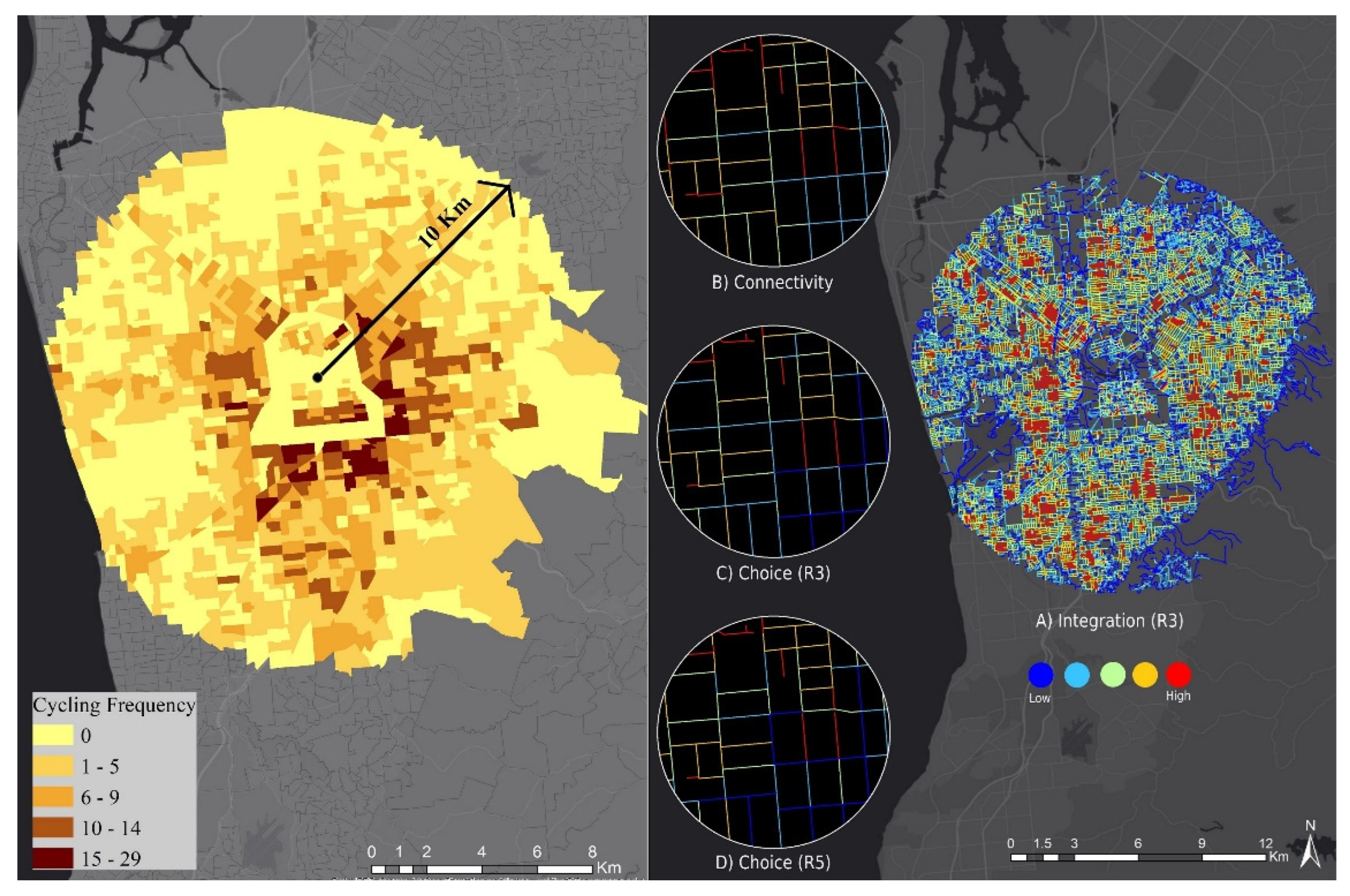
2.2. Study Area
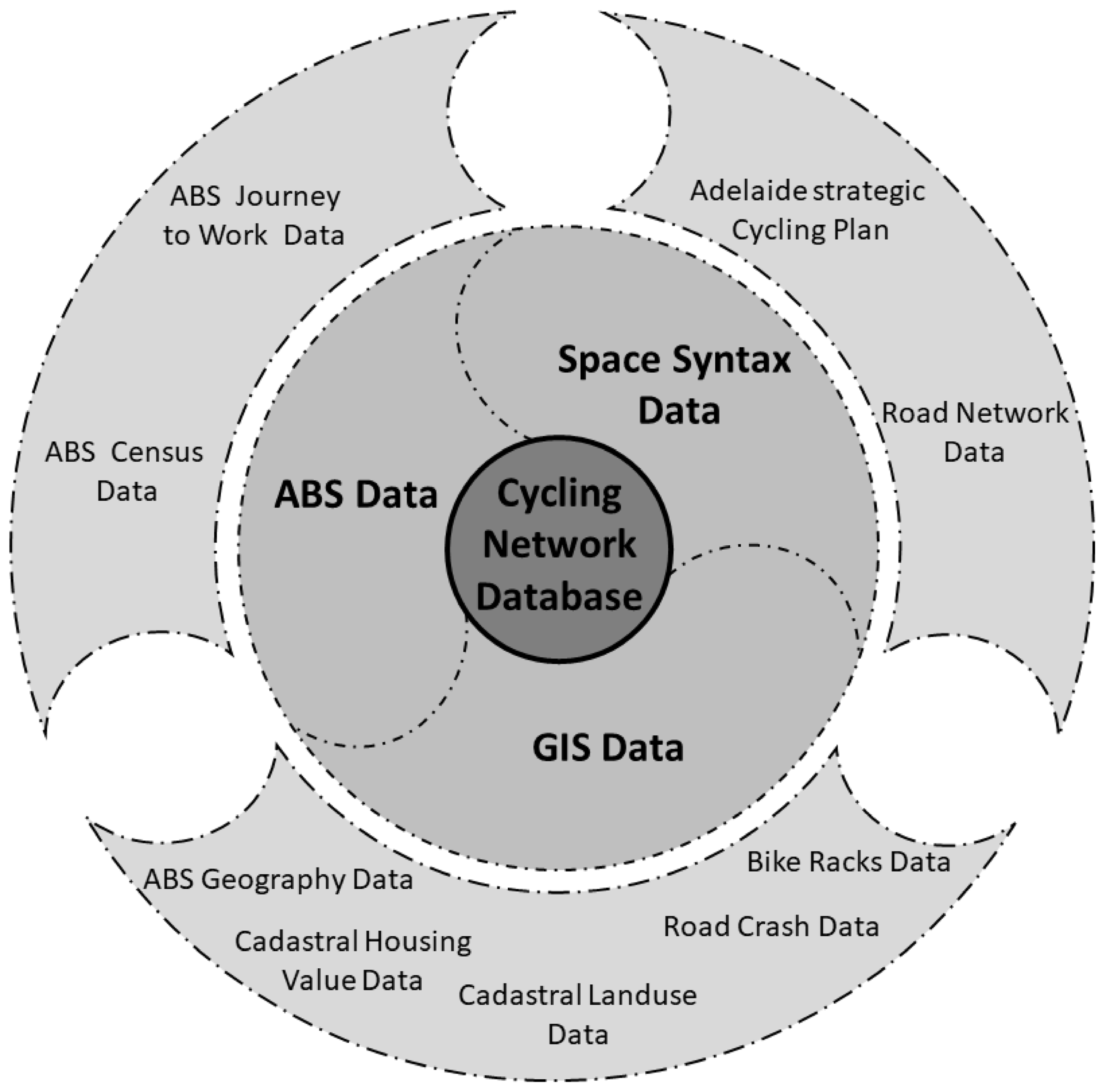
2.3. Data
3. Results
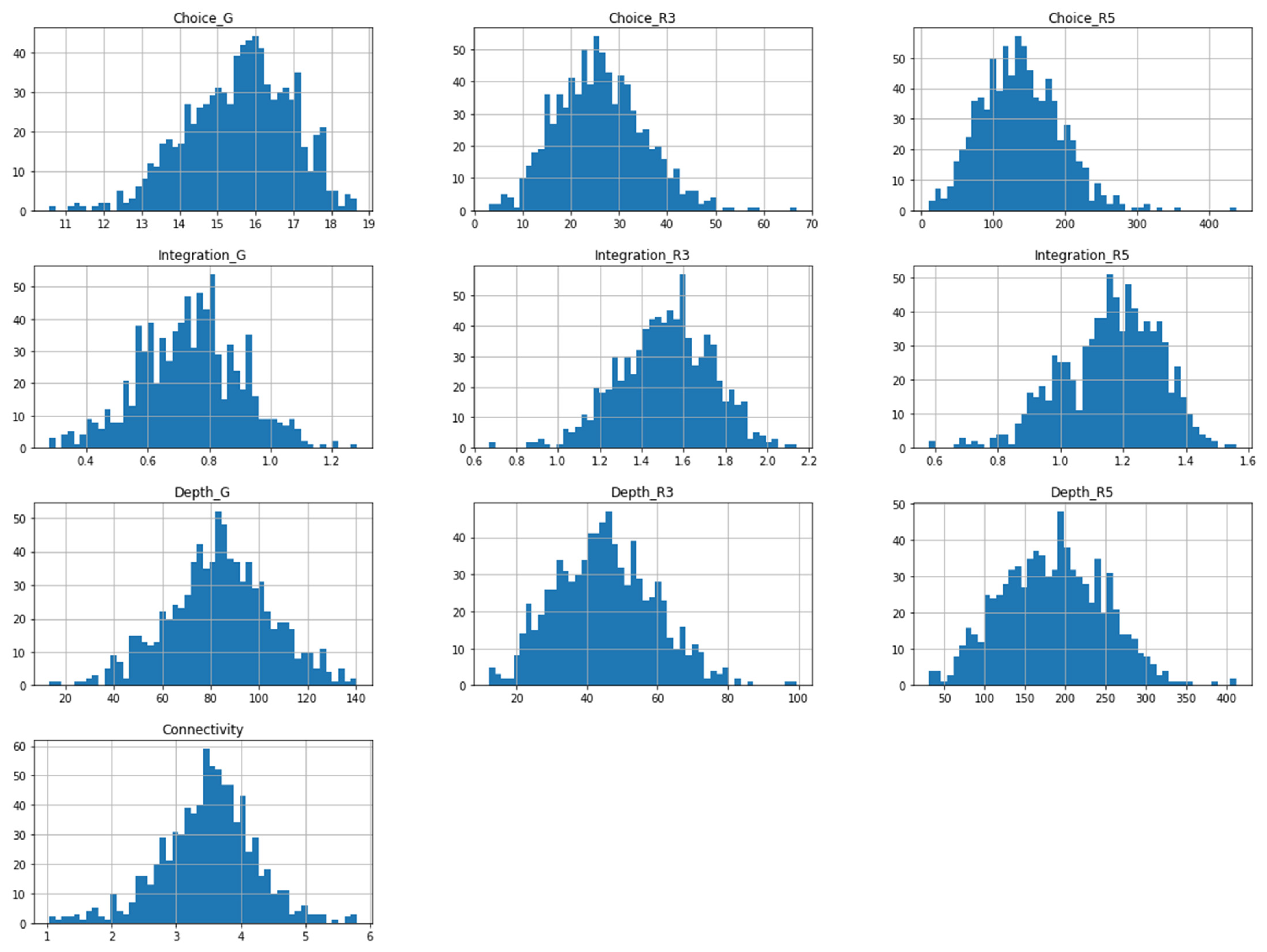
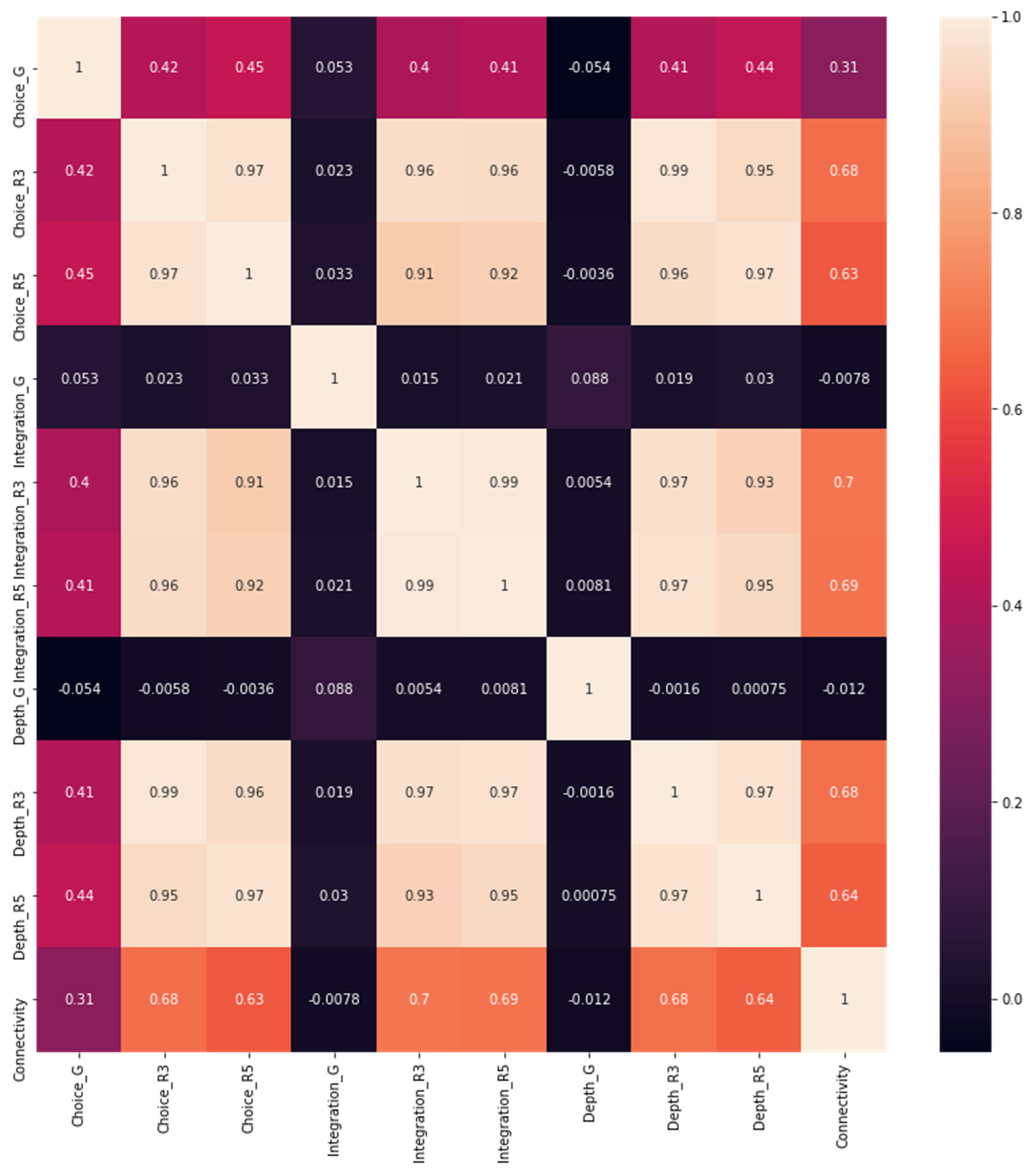
3.1. Correlation Analysis
3.2. Logarithmic-Transformed Regression
4. Discussion and Conclusions
Author Contributions
Funding
Institutional Review Board Statement
Informed Consent Statement
Data Availability Statement
Acknowledgments
Conflicts of Interest
References
- Law, S.F.; Karnilowicz, W. ‘In Our Country it’s Just Poor People who Ride a Bike’: Place, Displacement and Cycling in Australia. J. Community Appl. Soc. Psychol. 2015, 25, 296–309. [Google Scholar] [CrossRef]
- Pucher, J.; Buehler, R. City Cycling; MIT Press: Cambridge, MA, USA, 2012. [Google Scholar]
- Pucher, J.; Buehler, R. At the Frontiers of Cycling. Policy Innovations in the Netherlands, Denmark, and Germany. World Transp. Policy Pract. 2007, 13, 8–57. [Google Scholar]
- Dalton, N.S.; Peponis, J.; Conroy-Dalton, R. To tame a TIGER one has to know its nature: Extending weighted angular integration analysis to the descriptionof GIS road-centerline data for large scale urban analysis. In Proceedings of the 4th International Space Syntax Symposium, London, UK, 17–19 June 2003. [Google Scholar]
- Hillier, B.; Hanson, J. The Social Logic of Space; Cambridge University Press: Cambridge, UK, 1989. [Google Scholar]
- Atakara, C.; Allahmoradi, M. Investigating the Urban Spatial Growth by Using Space Syntax and GIS—A Case Study of Famagusta City. ISPRS Int. J. Geo-Inf. 2021, 10, 638. [Google Scholar] [CrossRef]
- Zhang, X.; Ren, A.; Chen, L.; Zheng, X. Measurement and spatial difference analysis on the accessibility of road networks in major cities of China. Sustainability 2019, 11, 4209. [Google Scholar] [CrossRef] [Green Version]
- Raford, N.; Chiaradia, A.; Gil, J. Space syntax: The role of urban form in cyclist route choice in Central London. In Proceedings of the TRB 2007 Annual Meeting Proceedings, Washington, DC, USA, 21–25 January 2007. [Google Scholar]
- Creutzig, F.; Javaid, A.; Soomauroo, Z.; Lohrey, S.; Milojevic-Dupont, N.; Ramakrishnan, A.; Sethi, M.; Liu, L.; Niamir, L.; Bren d’Amour, C. Fair street space allocation: Ethical principles and empirical insights. Transp. Rev. 2020, 40, 711–733. [Google Scholar] [CrossRef]
- Cooper, C.H. Using spatial network analysis to model pedal cycle flows, risk and mode choice. J. Transp. Geogr. 2017, 58, 157–165. [Google Scholar] [CrossRef]
- Pritchard, R.; Frøyen, Y.; Snizek, B. Bicycle level of service for route choice—A GIS evaluation of four existing indicators with empirical data. ISPRS Int. J. Geo-Inf. 2019, 8, 214. [Google Scholar] [CrossRef] [Green Version]
- Ashley, C.A.; Bannister, C. Cycling to Work from Wards in a Metropolitan Area. 1. Factors Influencing Cycling to Work. Traffic Eng. Control 1989, 30, 297–302. [Google Scholar]
- Strano, E.; Viana, M.; da Fontoura Costa, L.; Cardillo, A.; Porta, S.; Latora, V. Urban street networks, a comparative analysis of ten European cities. Environ. Plan. B Plan. Des. 2013, 40, 1071–1086. [Google Scholar] [CrossRef] [Green Version]
- Nelson, A.C.; Allen, D. If you build them, commuters will use them: Association between bicycle facilities and bicycle commuting. Transp. Res. Rec. 1997, 1578, 79–83. [Google Scholar] [CrossRef]
- Chen, C.-F.; Chen, P.-C. Estimating recreational cyclists’ preferences for bicycle routes–Evidence from Taiwan. Transp. Policy 2013, 26, 23–30. [Google Scholar] [CrossRef]
- Hunt, J.D.; Abraham, J.E. Influences on bicycle use. Transportation 2007, 34, 453–470. [Google Scholar] [CrossRef]
- Nikiforiadis, A.; Basbas, S. Can pedestrians and cyclists share the same space? The case of a city with low cycling levels and experience. Sustain. Cities Soc. 2019, 46, 101453. [Google Scholar] [CrossRef]
- Philips, I.; Clarke, G.; Watling, D. A fine grained hybrid spatial microsimulation technique for generating detailed synthetic individuals from multiple data sources: An application to walking and cycling. Int. J. Microsimul. 2017, 10, 167–200. [Google Scholar] [CrossRef]
- Campisi, T.; Acampa, G.; Marino, G.; Tesoriere, G. Cycling master plans in Italy: The I-BIM feasibility tool for cost and safety assessments. Sustainability 2020, 12, 4723. [Google Scholar] [CrossRef]
- Ratti, C. Space syntax: Some inconsistencies. Environ. Plan. B Plan. Des. 2004, 31, 487–499. [Google Scholar] [CrossRef]
- Nguyen, H.A.; Soltani, A.; Allan, A. Adelaide’s east end tramline: Effects on modal shift and carbon reduction. Travel Behav. Soc. 2018, 11, 21–30. [Google Scholar] [CrossRef]
- Soltani, A.; Allan, A.; Nguyen, H.A.; Berry, S. Bikesharing experience in the city of Adelaide: Insight from a preliminary study. Case Stud. Transp. Policy 2019, 7, 250–260. [Google Scholar] [CrossRef]
- Ogilvie, D.; Egan, M.; Hamilton, V.; Petticrew, M. Promoting walking and cycling as an alternative to using cars: Systematic review. BMJ 2004, 329, 763. [Google Scholar] [CrossRef] [Green Version]
- Rybarczyk, G.; Wu, C. Examining the impact of urban morphology on bicycle mode choice. Environ. Plan. B Plan. Des. 2014, 41, 272–288. [Google Scholar] [CrossRef]
- Lebendiger, Y.; Lerman, Y. Applying space syntax for surface rapid transit planning. Transp. Res. Part A Policy Pract. 2019, 128, 59–72. [Google Scholar] [CrossRef]
- Turner, A. From axial to road-centre lines: A new representation for space syntax and a new model of route choice for transport network analysis. Environ. Plan. B Plan. Des. 2007, 34, 539–555. [Google Scholar] [CrossRef] [Green Version]
- Kazerani, A. Characterization of the urban street network and its emerged phenomena. Master Thesis, University of Melbourne, Melbourne, Australia, 2010. [Google Scholar]
- Farahani, F.V.; Karwowski, W.; Lighthall, N.R. Application of graph theory for identifying connectivity patterns in human brain networks: A systematic review. Front. Neurosci. 2019, 13, 585. [Google Scholar] [CrossRef] [PubMed]
- van Nes, A.; Yamu, C. Space Syntax: A method to measure urban space related to social, economic and cognitive factors. In The Virtual and the Real in Planning and Urban Design; Routledge: London, UK, 2017; pp. 136–150. [Google Scholar]
- Javadpoor, M.; Soltani, A. The Effect of Individual and Socio-Economic Properties of Families and Street Configuration on the Walking of Elementary Students of Shiraz City. Phys. Sacial Plan. 2021, 8, 91–108. [Google Scholar] [CrossRef]
- Roosta, M.; Javadpoor, M.; Ebadi, M. A study on street network resilience in urban areas by urban network analysis: Comparative study of old, new and middle fabrics in shiraz. Int. J. Urban Sci. 2021, 18, 1–23. [Google Scholar] [CrossRef]
- Soltani, A.; Allan, A.; Pojani, D.; Khalaj, F.; Mehdizadeh, M. Users and non-users of bikesharing: How do they differ? Transp. Plan. Technol. 2022, 32, 39–58. [Google Scholar] [CrossRef]
- Australian Bureau of Statistics. 2016 Census QuickStats. 2016. Available online: https://www.abs.gov.au/websitedbs/D3310114.nsf/Home/2016%20QuickStats/ (accessed on 27 July 2021).
- South Austrilian Government Data Directly. Available online: https://data.sa.gov.au/ (accessed on 14 July 2021).
- SA, SAILIS. Available online: https://sailis.lssa.com.au/ (accessed on 25 July 2021).
- GitHub. DepthmapX-Multi-Platform Spatial Network Analyses Software. Available online: https://github.com/varoudis/depthmapX (accessed on 12 June 2021).
- Iacono, M.; Krizek, K.J.; El-Geneidy, A. Measuring non-motorized accessibility: Issues, alternatives, and execution. J. Transp. Geogr. 2010, 18, 133–140. [Google Scholar] [CrossRef] [Green Version]
- Australian Bureau of Statistics. Socio-Economic Indexes for Areas. Available online: https://www.abs.gov.au/websitedbs/censushome.nsf/home/seifa/ (accessed on 18 July 2021).
- Lovric, M. International Encyclopedia of Statistical Science; Springer Science & Business Media: Berlin, Germany, 2010. [Google Scholar]
- Leong, Y.-Y.; Yue, J.C. A modification to geographically weighted regression. Int. J. Health Geogr. 2017, 16, 11. [Google Scholar] [CrossRef] [Green Version]
- Soltani, A.; Pettit, C.J.; Heydari, M.; Aghaei, F. Housing price variations using spatio-temporal data mining techniques. J. Hous. Built Environ. 2021, 36, 199–1227. [Google Scholar] [CrossRef]
- Glen, S. “Welcome to Statistics How To!” from StatisticsHowTo.Com: Elementary Statistics for the Rest of Us! Available online: https://www.statisticshowto.com/ (accessed on 31 October 2021).
- Eldeeb, G.; Mohamed, M.; Páez, A. Built for active travel? Investigating the contextual effects of the built environment on transportation mode choice. J. Transp. Geogr. 2021, 96, 103158. [Google Scholar] [CrossRef]
- Handy, S.L.; Xing, Y. Factors correlated with bicycle commuting: A study in six small US cities. Int. J. Sustain. Transp. 2011, 5, 91–110. [Google Scholar] [CrossRef]
- Liu, J.H.; Shi, W. Impact of bike facilities on residential property prices. Transp. Res. Rec. 2017, 2662, 50–58. [Google Scholar] [CrossRef] [Green Version]
- Krizek, K.J. Two approaches to valuing some of bicycle facilities’ presumed benefits: Propose a session for the 2007 national planning conference in the city of brotherly love. J. Am. Plan. Assoc. 2006, 72, 309–320. [Google Scholar] [CrossRef]
- Schiff, N. Bike Lanes and Housing Prices, Commerce 407: Real Estate Economics. Research Report. City of Vancouver. 2020. Available online: https://www.nathanschiff.com/webdocs/c407_Winner_2013_Micu_etal.pdf (accessed on 25 July 2021).
- Flanagan, E.; Lachapelle, U.; El-Geneidy, A. Riding tandem: Does cycling infrastructure investment mirror gentrification and privilege in Portland, OR and Chicago, IL? Res. Transp. Econ. 2016, 60, 14–24. [Google Scholar] [CrossRef]
- Sener, I.N.; Eluru, N.; Bhat, C.R. Who are bicyclists? Why and how much are they bicycling? Transp. Res. Rec. 2009, 2134, 63–72. [Google Scholar] [CrossRef] [Green Version]
- Koohsari, M.J.; Oka, K.; Owen, N.; Sugiyama, T. Natural movement: A space syntax theory linking urban form and function with walking for transport. Health Place 2019, 58, 102072. [Google Scholar] [CrossRef]
- Ozbil, A.; Argin, G.; Yesiltepe, D. Pedestrian route choice by elementary school students: The role of street network configuration and pedestrian quality attributes in walking to school. Int. J. Des. Creat. Innov. 2016, 4, 67–84. [Google Scholar] [CrossRef]
- Schepers, P.; Lovegrove, G.; Helbich, M. Urban Form and Road Safety: Public and Active Transport Enable High Levels of Road Safety. In Integrating Human Health into Urban and Transport Planning: A Framework; Nieuwenhuijsen, M., Khreis, H., Eds.; Springer International Publishing: Cham, Switzerland, 2019; pp. 383–408. [Google Scholar] [CrossRef]
- Rybarczyk, G.; Ozbil, A.; Andresen, E.; Hayes, Z. Physiological responses to urban design during bicycling: A naturalistic investigation. Transp. Res. Part F Traffic Psychol. Behav. 2020, 68, 79–93. [Google Scholar] [CrossRef]
- Stein, P. Why are bike lanes such heated symbols of gentrification. Wash. Post 2015, 12. Available online: https://www.washingtonpost.com/news/local/wp/2015/11/12/why-are-bike-lanes-such-heated-symbols-of-gentrification/ (accessed on 15 August 2021).
- Ewing, R.; Schmid, T.; Killingsworth, R.; Zlot, A.; Raudenbush, S. Relationship between Urban Sprawl and Physical Activity, Obesity, and Morbidity. Am. J. Health Promot. 2003, 18, 47–57. [Google Scholar] [CrossRef]
- Parkin, J.; Wardman, M.; Page, M. Models of perceived cycling risk and route acceptability. Accid. Anal. Prev. 2007, 39, 364–371. [Google Scholar] [CrossRef] [PubMed] [Green Version]
- Dill, J.; McNeil, N. Four Types of Cyclists?: Examination of Typology for Better Understanding of Bicycling Behavior and Potential. Transp. Res. Rec. 2013, 2387, 129–138. [Google Scholar] [CrossRef] [Green Version]

| Region | Commuting Cycling | No. of Employed People | Commuting Cycling (Percent) | ||||||
|---|---|---|---|---|---|---|---|---|---|
| Male | Female | Total | Male | Female | Total | Men | Women | Total | |
| Greater Adelaide Metropolitan | 4368 | 1144 | 5512 | 334,036 | 222,691 | 556,727 | 1.31 | 0.51 | 0.99 |
| Variable name | Description | Count | Mean | Std | Min | Max |
|---|---|---|---|---|---|---|
| E_M25_34 | Number of male workers aged 25 to 34 | 822 | 26.35 | 16.05 | 8 | 186 |
| IER_Index | SEIFA advantage | 822 | 4.71 | 2.43 | 1 | 10 |
| LnCmmrcl | Commercial area (Ln) | 822 | 5.13 | 3.81 | 1 | 12.34 |
| LnEducnl | Educational area (Ln) | 822 | 3.10 | 3.57 | 1 | 13.17 |
| AvgP_Price | Average housing value multiplied (per $1000) | 822 | 4.11 | 0.86 | 2.13 | 9.56 |
| Sep_H | Number of separated houses | 822 | 93.82 | 29.72 | 0 | 131 |
| CBD_dummy | CBD area = 1, other = 0 | 822 | 0.43 | 0.49 | 0 | 1 |
| Connectivity | Space Syntax: Connectivity | 822 | 3.58 | 0.77 | 1 | 6 |
| Bike | Number of workers cycled to work | 822 | 5.95 | 3.07 | 3 | 22 |
| Variable | Coef. | Std. Err. | t-Statistic | p > |t| | [0.025 | 0.975] | VIF | Elasticity |
|---|---|---|---|---|---|---|---|---|
| const | −0.891 | 0.114 | −7.844 | 0 | −1.113 | −0.668 | - | - |
| E_M25_34 | 0.005 | 0.001 | 4.089 | 0 | 0.003 | 0.008 | 2.118 | 0.5 |
| IER_Index | 0.050 | 0.007 | 7.271 | 0 | 0.036 | 0.063 | 1.063 | 5.0 |
| LnCmmrcl | 0.008 | 0.004 | 2.061 | 0.04 | 0 | 0.017 | 1.762 | 0.008 |
| LnEducnl | 0.011 | 0.004 | 2.682 | 0.007 | 0.003 | 0.018 | 2.431 | 0.011 |
| AvgP_Price | 0.020 | 0.021 | 9.627 | 0 | 0.163 | 0.246 | 1.030 | 2.04 |
| Sep_H | −0.001 | 0 | −9.853 | 0 | −0.002 | −0.001 | 1.271 | −1.0 |
| CBD_dummy | 0.262 | 0.036 | 7.312 | 0 | 0.192 | 0.333 | 2.006 | - |
| Connectivity | 0.077 | 0.019 | 4.119 | 0 | 0.04 | 0.114 | 2.429 | 7.7 |
| R-squared | 0.505 | Omnibus: | 2.623 | |||||
| Adj. R-squared | 0.500 | Prob (Omnibus) | 0.269 | |||||
| F-statistic | 103.5 | Skew | −0.049 | |||||
| Prob (F-statistic) | 1.53 × 10−118 | Kurtosis | 2.757 | |||||
| Log-Likelihood | −408.74 | Durbin-Watson | 1.940 | |||||
| AIC | 835.5 | Jarque-Bera (JB) | 2.356 | |||||
| BIC | 877.9 | Prob (JB) | 0.308 | |||||
| No. Observations | 822 | Cond. No. | 3.88 × 10³ | |||||
Publisher’s Note: MDPI stays neutral with regard to jurisdictional claims in published maps and institutional affiliations. |
© 2022 by the authors. Licensee MDPI, Basel, Switzerland. This article is an open access article distributed under the terms and conditions of the Creative Commons Attribution (CC BY) license (https://creativecommons.org/licenses/by/4.0/).
Share and Cite
Soltani, A.; Allan, A.; Javadpoor, M.; Lella, J. Space Syntax in Analysing Bicycle Commuting Routes in Inner Metropolitan Adelaide. Sustainability 2022, 14, 3485. https://doi.org/10.3390/su14063485
Soltani A, Allan A, Javadpoor M, Lella J. Space Syntax in Analysing Bicycle Commuting Routes in Inner Metropolitan Adelaide. Sustainability. 2022; 14(6):3485. https://doi.org/10.3390/su14063485
Chicago/Turabian StyleSoltani, Ali, Andrew Allan, Masoud Javadpoor, and Jaswanth Lella. 2022. "Space Syntax in Analysing Bicycle Commuting Routes in Inner Metropolitan Adelaide" Sustainability 14, no. 6: 3485. https://doi.org/10.3390/su14063485
APA StyleSoltani, A., Allan, A., Javadpoor, M., & Lella, J. (2022). Space Syntax in Analysing Bicycle Commuting Routes in Inner Metropolitan Adelaide. Sustainability, 14(6), 3485. https://doi.org/10.3390/su14063485