Improving Air Quality in Urban Recreational Areas through Smart Traffic Management

Abstract

Green parks are the only natural places for recreation in many metropolitan areas, and the European Commission is seeking to improve their air quality and, consequently, citizens’ physical and mental health. One of the recently adopted approaches is to achieve pollution abatement in these green areas by reducing nearby traffic. In this paper, we analyze the impact of reducing the traffic in nearby streets to avoid pollution by proposing two different approaches. Our goal is to improve the pollution levels in Valencia’s most significant green areas by limiting vehicular traffic flow in nearby streets. To this end, we consider two alternative solutions—a more restrictive one and a less restrictive approach—in an attempt to achieve a tradeoff between emission control and congestion avoidance. Moreover, we show how our proposal can reroute traffic throughout the city without having traffic jam problems associated with the proposed approaches. In addition, we determine how the traffic flow data and the emissions in the city vary due to the traffic restrictions that we enforce. The experimental results show that it is possible to achieve improvements in terms of pollution with both of our restriction approaches; in particular, with the partial traffic isolation model, the pollution rates in the target area decreased by 17%, which we consider an excellent initial result for the applicability and effectiveness of these methods when an adequate traffic routing system is adopted.

1. Introduction

Traffic jams associated with the use of private vehicles in large cities are a common phenomenon. In addition to causing stress and other personal discomfort, they also lead to an increase in air pollutant concentrations [1]. Valencia is the fourth city in Spain in terms of traffic congestion according to data from the “Traffic Index TomTom 2020” report [2], which analyzes traffic jams and traffic volumes in 416 cities around the world, 25 of which are in Spain. Data are obtained from more than 600 million drivers who use TomTom technology in their navigation devices. All of the data provided represent (as a percentage) how much extra time it takes to complete an average journey that would take 30 min without traffic.

In terms of health, data from the Spanish Society of Pneumology and Thoracic Surgery (SEPAR) [3] show that pollution generates 10,000 deaths per year in Spain and 7 million around the world, and emissions of polluting gases produced by traffic are one of the main causes. Traffic jams are responsible for most of the pollution in large cities due to the high concentration of vehicles and their stop-and-go traffic.

With the objective of reducing air pollutant concentrations, some cities have taken specific actions—for example, Valencia in Spain. Its strategies to achieve this goal are detailed in its Sustainable Urban Mobility Plan (Plan de Movilidad Urbana Sostenible) [4]. This plan takes pedestrians, bicycles, public transport, and private vehicles into account. Firstly, for pedestrians, walking is promoted and the area of pedestrian spaces in the city is recovered and enlarged. Second, for bicycles, adequate infrastructure is ensured and the city’s cycling network is improved. Third, for public transport, the network is adapted to the new mobility needs of citizens. Fourthly, for private vehicles, road hierarchies are introduced to prioritize public transport (bus/taxi lanes), traffic speed is reduced to a maximum of 30 km/h in different neighborhoods of the city, access to certain areas is forbidden for non-resident vehicles, and the space dedicated to parking is reorganized. Finally, in a cross-cutting manner, the “Smart City” concept is enhanced through real-time mobility management.

In terms of future challenges, according to the European Commission’s action plan [5], by 2030, the EU should reduce the health impact of air pollution by more than 55% (e.g., premature deaths). With regard to reducing the emissions of road transport, the EU, in line with what it did regarding CO${}_2$ emissions, will consider the need to limit PM2.5 emissions from all types of combustion engines and from the brakes of conventional and electric vehicles alike. The Commission also intends to promote depolluted and re-naturalized sites as potential public green spaces with the intention of improving the mental and physical wellbeing of the population.

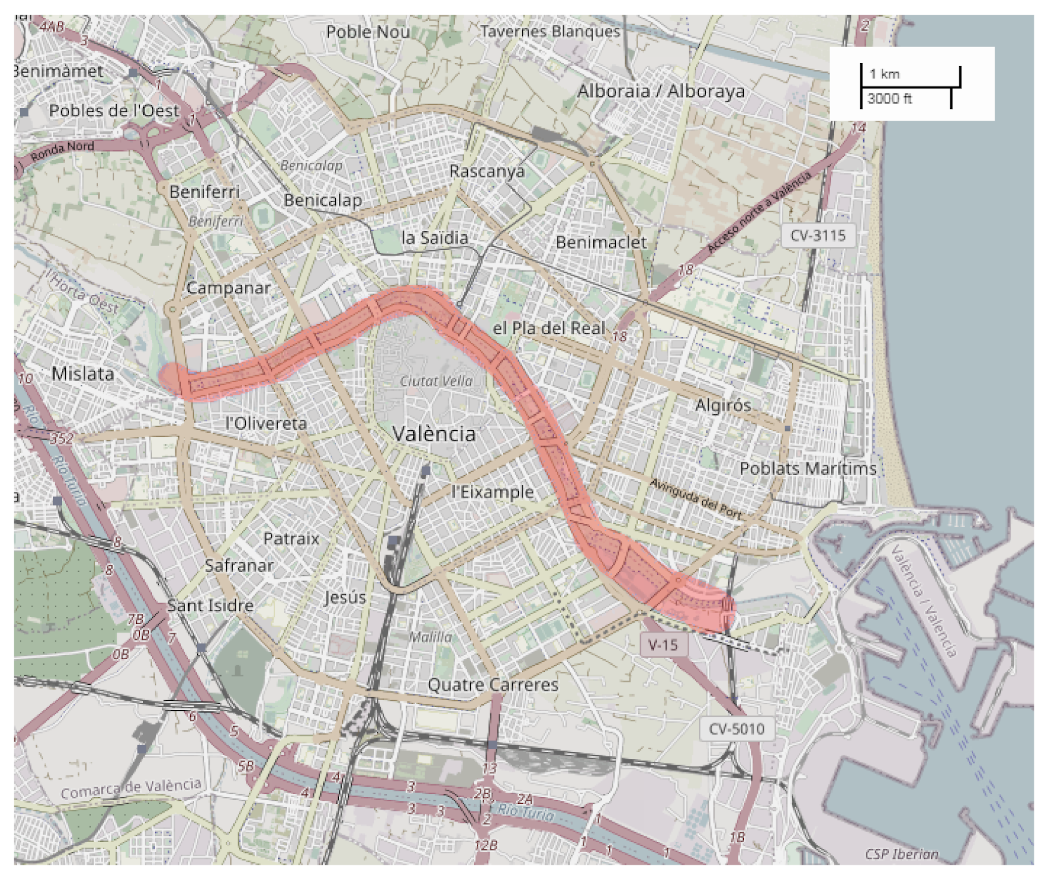
In this work, we intend to go one step further by considering more restrictive measures for traffic flow in order to safeguard the health of citizens. In particular, we will focus on the main recreational and green areas of Valencia, which belong to the old riverbed (see Figure 1) that has been converted into the biggest green area of the city, fully spanning from west to east, up to the seaside.

Figure 1. Old riverbed of Valencia (highlighted in red).

Since this area is concentrated with many citizens that perform physical and leisure activities throughout the day and many small children who are also playing, it is of utmost importance for authorities to guarantee that the air quality levels in this area are as good as possible. In this regard, any solution that reduces the amount of traffic flowing near this green area is welcome. In this work, we will consider two alternative solutions—a more restrictive one, where traffic flow near the target area is completely avoided, and a less restrictive approach, where traffic is allowed, but only at selected locations (bridges that cross the old river)—in an attempt to achieve a tradeoff between emission control and congestion avoidance. Hence, the main goal of the current work is to study the most adequate solution for improving the air quality in the aforementioned green areas of the city by controlling traffic in a way that minimizes the environmental impact on that area while maintaining similar travel times; in addition, we seek to avoid a negative impact by excessively congesting or increasing pollution emissions in other parts of the city. A detailed study based on our realistic simulation framework shows that, between the two alternatives that we propose for restricting traffic, the less restrictive one offers an adequate balance between pollution emissions in the target area and travel time increase. In particular, experiments show that we are able to reduce the average presence of different pollutants in the target area by 17% while introducing a very minor increase in the other areas, which is 49% in the worst case detected overall.

Finally, the rest of this paper is organized as follows: In Section 2, we present some related work in this research area. Afterward, in Section 3, we present our proposal for addressing this problem. Simulation results are then presented and discussed in Section 4. Finally, the main conclusions are presented in Section 5, along with references to future work.

2. Related Work

In this section, we will discuss some academic work that is related to our project.

In [6], Afrin and Yodo provided a survey where they analyzed the current challenges in measuring traffic congestion. Throughout the survey, they examined the main causes of congestion and described the different categories used to measure congestion. Then, through the use of a traffic dataset, they examined all of the categories for congestion level measurements. Finally, they referred to established criteria for good congestion measurement and detailed current approaches to congestion mitigation. In general terms, it was a solid survey that analyzed many aspects related to congestion. However, unlike our study, it did not analyze any parameters related to pollution—neither pollutant emissions nor Air Quality Index (AQI) values.

In [7], Doolan and Muntean presented a vehicle-routing solution for reducing carbon dioxide emissions without significantly affecting travel times. The model is called EcoTrec, and it is based on a VANET where vehicles exchange messages related to traffic and road conditions, such as the average speed on the road. After getting the necessary information, a fuel-efficiency model is built and, due to this, less greenhouse pollutants are emitted, while low traffic congestion levels are maintained. Their architectural model consists of the EcoTrec routing engine and three different models: vehicle, road, and traffic. The EcoTrec engine has the aim of calculating the most fuel-efficient route by looking at the efficiency of individual road segments while considering different factors: road condition, traffic condition, and the weight of the road. In terms of results, their solution showed an average reduction of fuel consumption comparable to that of other algorithms while maintaining the traffic flow conditions. On the contrary, for traffic congestion situations, their solution was not appropriate because the vehicles calculated alternative routes on their own without considering the neighbors’ routes, which led to the maintenance of the overall congestion levels. In addition, they did not measure the different pollutant metrics (only CO${}_2$), so they were not as thorough as we are in our work. Furthermore, they did not use a model to measure air pollutant concentrations and, consequently, AQI levels.

iMOB is an intelligent urban MOBility management system that was proposed by Akabane et al. [8]. The project is based on applying the Vehicular Social Network (VSN) concept and analyzing the impact of using the Social Network Analysis (SNA) and Social Networking Concept (SNC) measures for urban traffic flow. At the same time, its architecture is based on a three-level system (classified from bottom to top): environment sensing, vehicle-ranking mechanism, and altruistic rerouting decisions. Environment sensing is responsible for obtaining the local awareness through vehicle crowd-sensing, and it enables users of a VSN to solve problems in collaboration with each other. The vehicle-ranking mechanism selects the best-located vehicle in the network based on the communication links between the vehicles. Then, the selected vehicle is responsible for the information aggregation and knowledge generation processes. Finally, the altruistic rerouting decision performs the vehicle-rerouting strategy in a collaborative way in order to avoid congestion spots. The paper’s results show that the use of social interactions and a virtual community in the vehicular environment helps to reduce the average travel time and CO${}_2$ emissions; nevertheless, they did not study other pollutants, average speed, or traveled distance. Moreover, they did not measure air pollutant concentrations; hence, they could not obtain AQI values and relate them to the AQI table.

SmartFlow is a VANET protocol that was proposed for V2I communications by Khan and Koubaa [9]. The main goal is to avoid long waiting delays due to traffic signals, and, for this purpose, it defines a protocol that can detect congestion and suggests to vehicles the optimal speed for circulating and for crossing traffic signals before they become red. All of this can be done by frequently sending beacon messages to other vehicles and Roadside Units (RSUs). The protocol system model is three-legged, and it includes a vehicle model, road model, and vehicular mobility model. The vehicle model assumes that all vehicles are intelligent and able to communicate to each other and with the RSU through a wireless transceiver. The road model aims at transmitting the characteristics of each road segment (road length, speed limit, number of lanes, number of RSUs, etc.) to vehicles. The vehicular mobility model is the car-following model, which primarily enforces the rule of keeping a safe distance ahead. In terms of results, the protocol performs well compared to others in the paper. In contrast, and unlike in our work, this system can only be implemented when vehicles are 100% autonomous, meaning that it is not applicable for the present day. Our work also differs from theirs because we measure environmental parameters, such as AQI levels, and evaluate the behavior of our model based on these parameters.

In [10], Gomides et al. presented REACT, a traffic management solution with the aim of minimizing vehicle congestion in smart cities. For this purpose, they suggested a VANET based on a V2V network architecture, where vehicles behave as intelligent agents, as they are able to process and transmit information among themselves. Communication is rooted in two phases: request and response. For the request phase, vehicles must ask for information about the displacement in neighboring road segments. For the response phase, the vehicles present on these roads must reply with their displacement analyses. This is a good solution for reducing communication overhead, and their results also showed a good performance in terms of travel time. Nevertheless, this approach seems to be optimistic because they do not use real traffic traces for the experiment. In addition, they also failed to analyze pollutant emissions and air pollutant concentrations.

Akabane et al. [11] presented a novel distributed traffic management system called dEASY (distributed vEhicle trAffic management SYstem). This is an infrastructure-less system based on a three-layer architecture that consists of environment sensing and vehicle ranking, knowledge generation and distribution, and knowledge consumption. The environment-sensing and vehicle-ranking layer collects raw traffic data in real time, such as position and speed, so that it becomes possible to extract from them an accurate knowledge about the traffic conditions of the roads. The knowledge generation and distribution layer deals with processing and aggregation of the raw data. In this layer, the individual raw data provided by the environment-sensing and vehicle-ranking layers are gathered and grouped until new knowledge comes out. In addition, this layer also delivers services to customers, e.g., route suggestions. Finally, the knowledge consumption layer provides a knowledge-based decision. This decision can have two approaches: selfish (decisions are made to seek your own benefit) and altruistic (decisions are made to seek the benefit of the overall system). The results show that the system performs well in terms of travel time and CO${}_2$ emissions. However, their approach is not as explicit as ours because they only measured CO${}_2$, failing to study other important pollutants, such as particulate matter or nitrogen oxide emissions. In addition, they also failed to study the various concentrations of the pollutants and their respective AQI values.

Finally, Table 1 shows a summary of which topics are covered in each work when compared to our own. Here, we can see that, in our work, in addition to dealing with traffic congestion problems, we also deal with emissions. Specifically, we improve the air quality of a selected area. We know that this improvement exists because we analyzed and measured different pollutants and used a model to obtain the air quality and, therefore, the AQI.

Table 1. Summary of the topics covered by the various related works and by our work.

Topics	[6]	[7]	[8]	[9]	[10]	[11]	Our Work
Deals with traffic congestion?	✓	✓	✓	✓	✓	✓	✓
Uses real traffic traces?	✓	✓	✓	✓	✗	✓	✓
Deals with emissions?	✗	✓	✓	✗	✗	✓	✓
Reduces emissions?	N.A. ${}^1$	✓	✓	N.A.	N.A.	✓	✓
Measures more than one pollutant?	N.A.	✗	✗	N.A.	N.A.	✗	✓
Measures air pollutant concentration?	N.A.	✗	✗	N.A.	N.A.	✗	✓
Measures AQI?	N.A.	✗	✗	N.A.	N.A.	✗	✓

¹ Not available.

3. Proposed Solution

Our proposed solution is based on previous works [12,13] and can adapt to all traffic constraints established by city administrations based on environmental criteria. Unlike the previous implementation, in this one, we can vary the weights of multiple streets, so we can perform new actions (i.e., vary the traffic flow and the amount of pollutants in an area). In common with that work, we have that the main core of the algorithm (Equation (1) and the ABATIS architecture) is kept intact, since its effectiveness was demonstrated. Hence, our main objective is to study the effect that these restrictions have on the air quality of the studied area and on the general traffic flow, taking as a reference the city of Valencia, Spain.

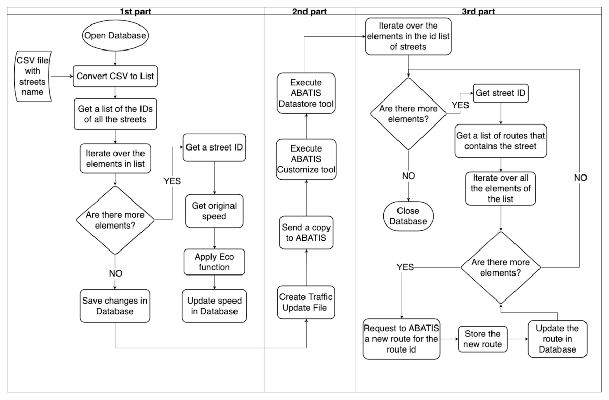
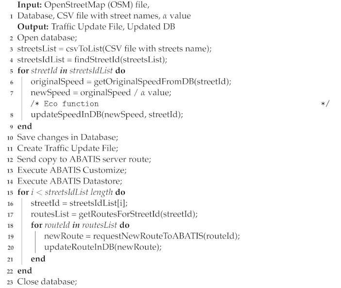
In a previous work, we presented a route server named Automatic Balancing of Traffic through the Integration of Smartphones with vehicles (ABATIS) [14], which allows us to centrally manage all of the traffic in a city in an efficient manner. When ABATIS is running, the overall behavior of our algorithm is the one shown in the process flow diagram presented in Figure 2. As can be seen, it first deals with the updating of speed values in street segments (lines 1 to 9); in particular, streets that are selected as belonging to critical areas experience an (artificial) reduction of their default speed that affects route computation, thereby minimizing the traffic flow through them. Secondly, the ABATIS part (lines 10 to 13) is responsible for updating the database with the new costs and for preparing the application for serving optimal routes. Finally, it handles requests for new routes and updates them in the database (lines 14 to 22) so that previous requests are taken into account for successive requests, thus achieving load balancing. Having said this, we will proceed to explain the first functionality in more detail, as it is the key part of our algorithm.

Algorithm 1 Proposed eco algorithm for enforcing traffic restrictions.

Figure 2. Process flow diagram of Algorithm 1.

First, we read the input file with the names of the streets. Afterwards, we apply a function that searches for each street name and converts it into an ‘id’. With the aim of applying our Equation (1), an iteration over all of the ids takes place. This equation changes the traffic weights of the different street segments by dividing the default velocity (V) by the factor $\alpha$. This is done in order to artificially reduce the speed of a street segment. Finally, all of the speed values are updated in the database. This is needed to create the Traffic Update File, which is necessary for updating the costs of the routes and, thus, obtaining new routes.

$$f\left(\alpha \right) = \frac{V}{\alpha }$$

(1)

ABATIS [14] is a routing server based on the Open-Source Routing Machine (OSRM) [15], and it is implemented in C++, as it is open source. As input data, it uses the files generated by OpenStreetMap in both PBF and OSM XML format. The access to the route information is done through HTTP requests. At the same time, ABATIS also implements different tools that can be used to modify the weights of the routes.

Regarding the pollutant assessment, on the one hand, we will only analyze three out of five pollutants present in the SUMO [16] emissions section: particulate matter (PM${}_x$), nitrogen oxides (NO${}_x$), and carbon monoxide (CO), as they are included in the World Health Organization (WHO) air quality guidelines [17] and in the directives of both the European Union [18] and the United States Environmental Protection Agency (USEPA) [19]. On the other hand, we will take into consideration the aggregated emissions of each edge/street and not the emissions of each vehicle, as this is a better approach than measuring the air quality.

Regarding the generation of pollutants, we will use three main elements: Firstly, for the vehicle creation, we rely on the real traffic traces obtained by Zambrano-Martinez et al. [20]; secondly, for the vehicle emission model, we adopt the HBEFA3 [21] model presented in SUMO; finally, concerning the profile of passenger cars within the province of Valencia, it was retrieved from the Spanish Department of Traffic or Dirección General de Tráfico (DGT) from their 2019 annual table statistics [22]. Focusing on the latter, the data can be organized according to two different criteria: the type of fuel or an environmental label [23]. As these do not meet our requirements, we combined both tables and obtained a vehicle distribution according to fuel type and HBEFA3 emission class (see Table 2). As can be seen, for our experiments, we had 45% gasoline cars (23% with a B tag and 22% with a C tag) and 55% diesel cars (28% with a B tag and 27% with a C tag).

Table 2. Estimation of the vehicles’ distribution in Valencia according to their profiles.

Vehicle Type	Emission Class	Volume (%)
Gasoline B	PC_G_EU3	23
Gasoline C	PC_G_EU5	22
Diesel B	PC_G_EU4	28
Diesel C	PC_G_EU6	27

In order to determine whether our solution is able to improve the air quality in our target area (city of Valencia), we are forced to use an air concentration model because SUMO only provides the emissions expressed in mass units, i.e., mg, and the pollutants in the AQI [24] tables [25] are expressed as the mass divided by the volume, i.e., μg/m³. For this purpose, we used the “Fixed Box Model” approach [26,27], which is a straightforward atmospheric dispersion model that consists of fitting the area to be studied—in our case, the city of Valencia and its old riverbed—into a parallelepiped. Equation (2) is used to calculate the concentration, where C is the average concentration of the given pollutant throughout this box, expressed in μg/m³; Q is the emission rate of the gas, or particles, expressed as the mass divided by the area; t is the time period over which mixing takes place (typically 1 h); finally, x, y, and z refer to the length, width, and height of the parallelepiped, respectively.

$$C = \frac{Q · t}{x · y · z}$$

(2)

To relate the concentration values to the AQI table, we will rely on Equation (3) [25], where $I_p$ is the index for pollutant p; $C_p$ is the truncated concentration of pollutant p; $B{P}_{Hi}$ is the concentration breakpoint that is greater than or equal to $C_p$; $B{P}_{Lo}$ is the concentration breakpoint that is less than or equal to $C_p$; $I_{Hi}$ is the AQI value corresponding to $B{P}_{Hi}$; $I_{Lo}$ is the AQI value corresponding to $B{P}_{Lo}$.

$$I_p = \frac{I_{Hi} - I_{Lo}}{B{P}_{Hi} - B{P}_{Lo}} · (C_p - B{P}_{Lo}) + I_{Lo}$$

(3)

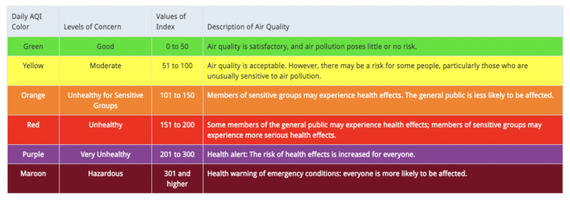
Finally, to obtain the global AQI level, the average integer value of the total indexes is calculated, so $I = avg(I_{PMx},I_{CO},I_{NOx})$, where I is the general AQI for the selected area. The different AQI levels are shown in Figure 3 and, as can be seen, there are six. They range from good to hazardous. Each one has a corresponding color, a description of the air quality, and an index range. In our case, we tried to keep the general index (I) below 51 points, which would give us a good air quality level.

Figure 3. AQI level table.

4. Simulation Results

In our case, we will analyze the effectiveness of our proposed solution in reducing the pollution rates and improving the air quality in the main green area of the city of Valencia, the old riverbed (see Figure 1), which has an extension of 1,110,000 m${}^2$ and a number of 7,000,000 visitors per year.

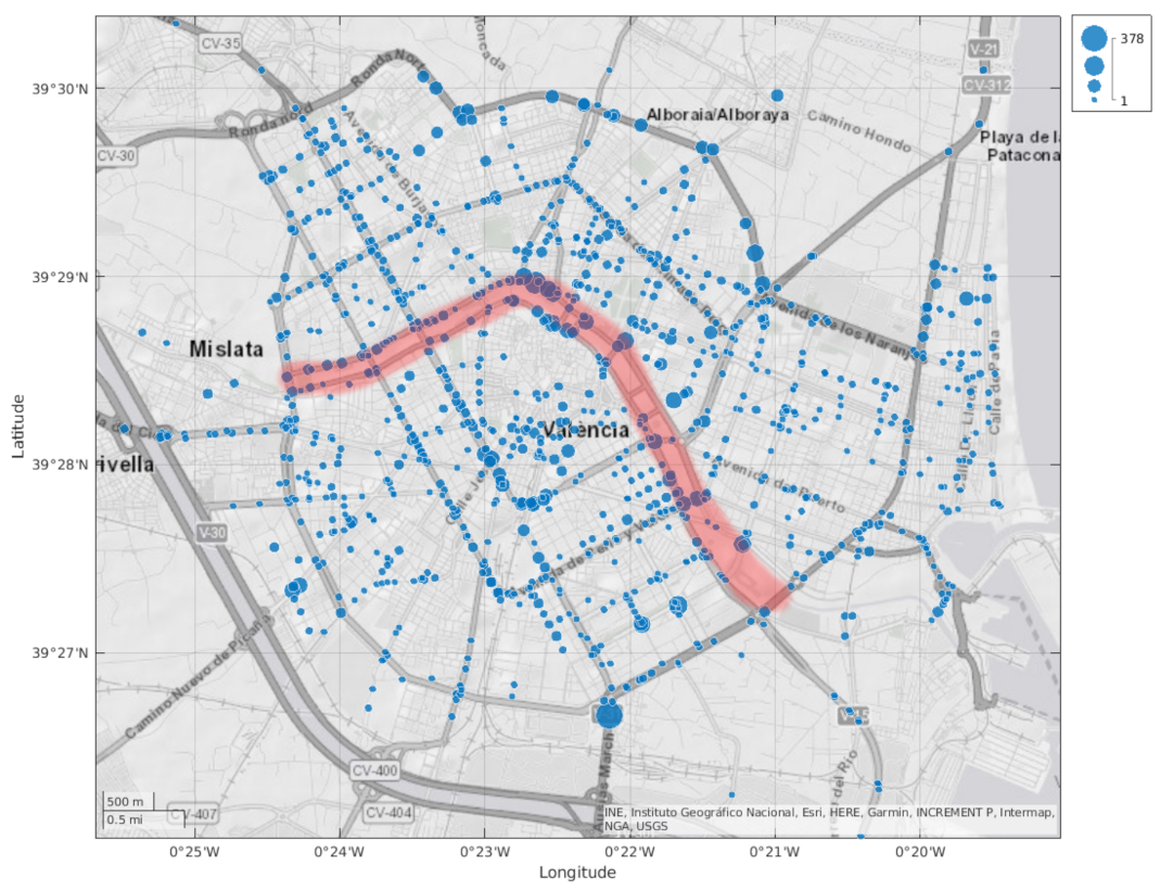
To accomplish the study, we built a set of vehicles that departed from various points of the city in order to have more representative data. These sources’ points are depicted in Figure 4, and, as it can be seen, they are well distributed throughout the city, so they are representative of real situations. According to the traffic information that Zambrano-Martinez et al. obtained in [20], which represents the traffic throughout the city on a working day from 8 until 9 a.m., in our experiment, 18,000 vehicles were circulating during a 15 min period.

Figure 4. Simulation traffic sources are marked in blue, and the target area (old riverbed) is highlighted in red.

Concerning the calculation of the air quality (AQI levels), we will apply the “Fixed Box Model” that was described before. For the old riverbed, we will use its area (1,100,100 m${}^2$) as the XY area of the box, and for the height we will consider a value of 20 m.

Having taken that into account, on the one hand, we will start by analyzing the full traffic isolation model in terms of average variation of pollutants for different $\alpha$ values, the AQI level for each pollutant, and, in general, the difference in the distribution of pollutants within the city when comparing the best result to the default situation. Then, on the other hand, we will analyze the same aspects for the partial traffic isolation model. Finally, we will compare the best results of both models.

4.1. Full Traffic Isolation

As previously mentioned, for the full traffic isolation model, we will increase the $\alpha$ parameter from 1 to 3.5 ($\alpha = 1$ is the default situation) for all streets and bridges near the old riverbed. With this scheme, we can observe how pollutants vary for different $\alpha$ values and determine which one is the best in terms of emission reduction.

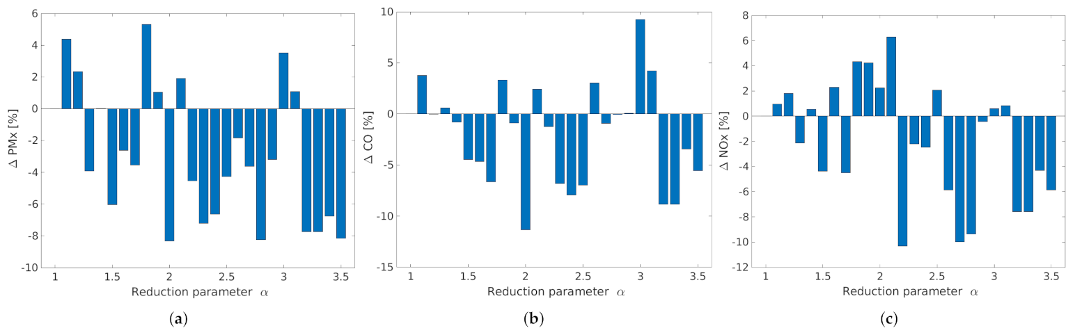
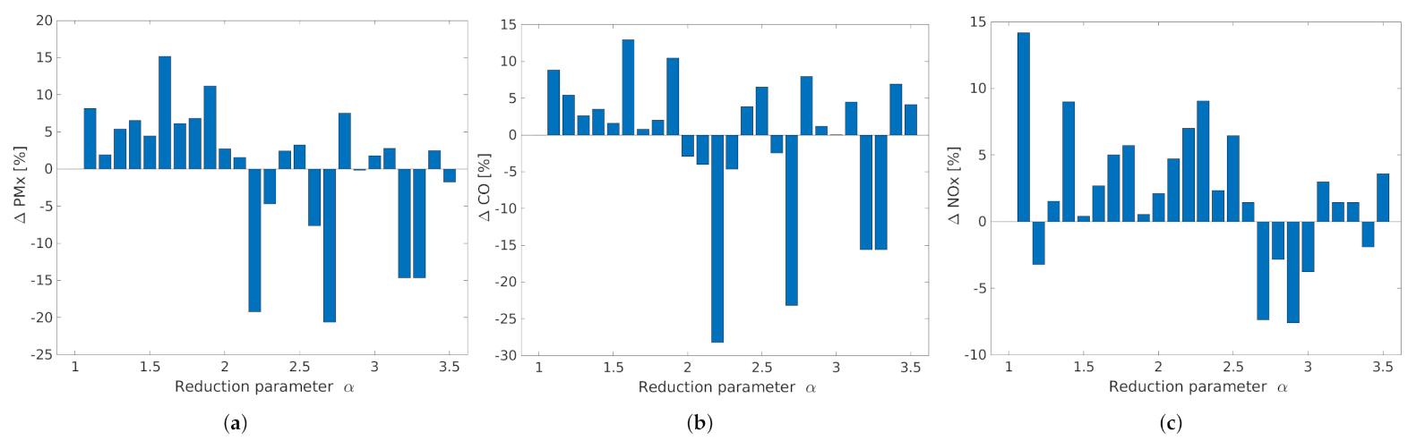
The results regarding the variation of the average pollutant emissions in the old riverbed with respect to normal (in terms of percentage) are shown in Figure 5. Specifically, in Figure 5a, we observe that the values $\alpha = 2;2.8;3.5$ achieve the best results with a decrease of about 8% in PM${}_x$ emissions whereas for $\alpha = 1.1;1.8$, there is an increase of about 5%. For the CO results, we observe in Figure 5b that, for $\alpha = 2$, there is a reduction of emissions of about 10%; conversely, for $\alpha = 2.9$, there is an increase of 10%. Finally, in terms of NO${}_x$ emissions, we observe in Figure 5c a reduction of about 10% for $\alpha = 2.2;2.7$, while for $\alpha = 2.1$, it increases by 6%.

Figure 5. Difference in pollutants in the old riverbed with respect to the default case for various $\alpha$ values (full traffic isolation). (a) PM${}_x$. (b) CO. (c) NO${}_x$.

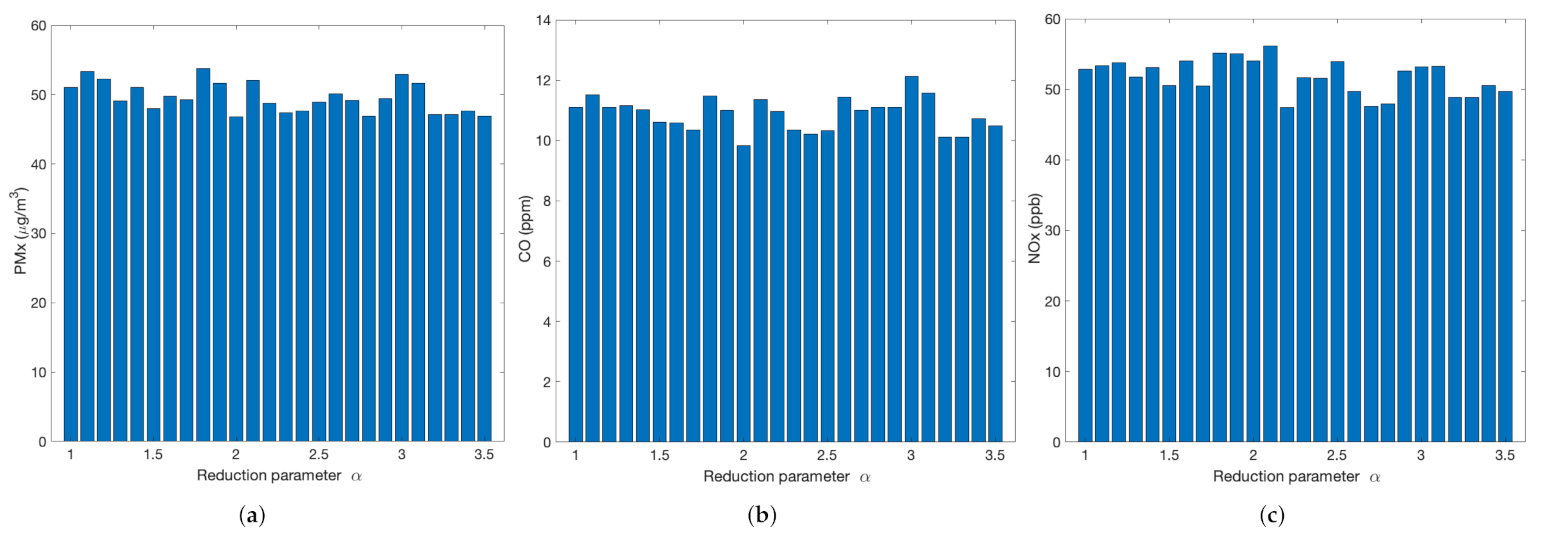
Since the average pollution difference is not a definitive way to determine which $\alpha$ is the best one, we will apply the ‘Fixed Box Model’ in order to obtain the AQI level for the selected area. To this end, we will consider t = 1 h for NO${}_x$, t = 8 h for CO, and t = 24 h for PM${}_x$. Based on these assumptions and the ones mentioned above, we obtain three figures of concentrations (see Figure 6a–c) for each $\alpha$. As shown, in terms of PM${}_x$ concentration, the best results are obtained for the same $\alpha$ as for the average variation (2; 2.8; 3.5), and the same occurs for the worst ones. Similar results are obtained for CO and NO${}_x$ in terms of both the best and worst results. Since this was expected, we will now analyze the results in terms of AQI, as this is the best way to determine which $\alpha$ is the best.

Figure 6. Concentrations of pollutants for each $\alpha$ in the old riverbed (full traffic isolation model). (a) PM${}_x$. (b) CO. (c) NO${}_x$.

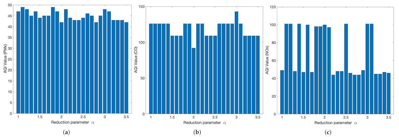
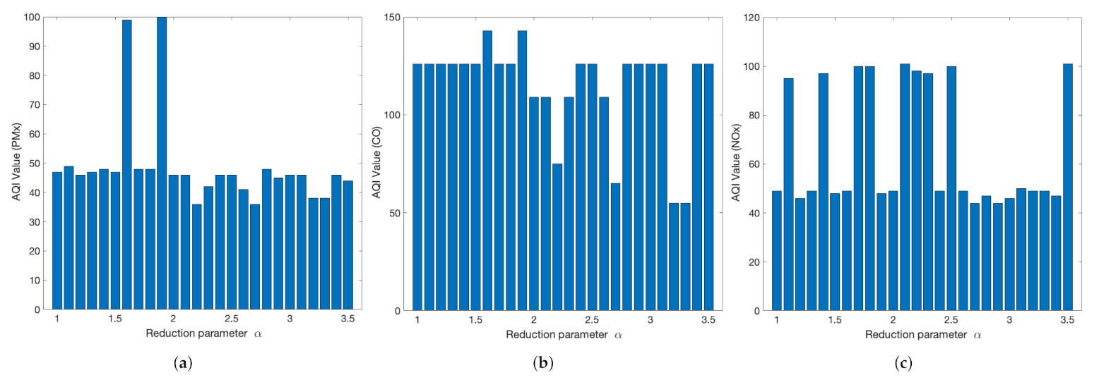
To obtain the AQIs for each pollutant and $\alpha$, we will use the concentration values, Equation (3), and the AQI table [25]. After performing some calculations, Figure 7a–c are obtained. As can be seen, the best AQIs for the old riverbed area are obtained for PM${}_x$ and some $\alpha$ of NO${}_x$, while the worst ones are obtained for CO and the other $\alpha$ of NO${}_x$. From all of them, we will obtain the overall AQI of the target area, since, as mentioned above, the overall AQI is computed as the average of the different pollutants’ AQIs.

Figure 7. AQI for each pollutant and $\alpha$ value in the old riverbed (full traffic isolation model). (a) PM${}_x$. (b) CO. (c) NO${}_x$.

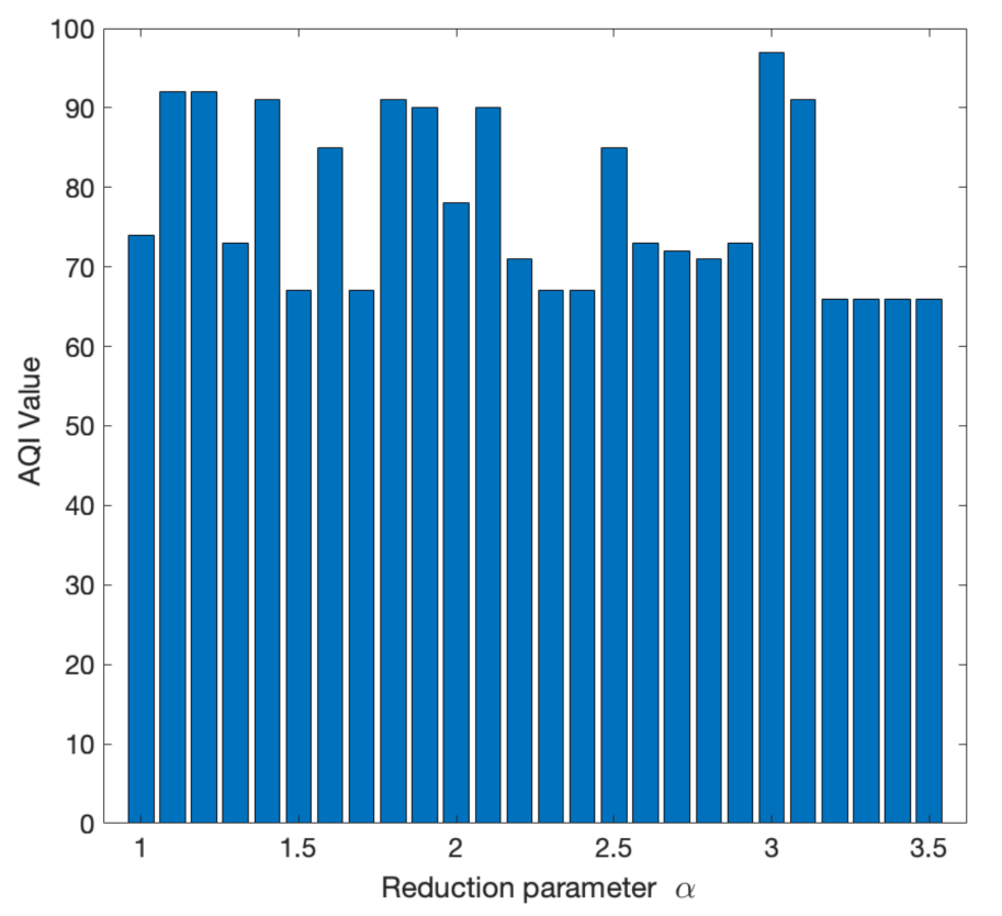
Figure 8 shows the different AQIs obtained in the old riverbed for each $\alpha$ value. We can see that there are many values as results of the experiments. The best alphas ($\alpha = 3.2;3.3;3.4;3.5$) have better values than the default situation ($\alpha = 1$), with AQIs of 66 and 74, respectively. The worst alpha value ($\alpha = 3$) has an AQI of 98, which represents an increase of 24 with respect to the default case. This way, we will now focus on the alpha with the best AQI in the old riverbed and with a smaller amount of pollutants. In particular, the solution with an alpha of 3.3 is selected. Focusing on how it performs in the city, this $\alpha$ has an average decrease of 1.58% in the amount of pollutants with respect to the normal value. We can conclude that $\alpha = 3.3$ achieves the best AQI results because it insignificantly increments the amount of pollutants in the city while reducing such levels in our target area, as intended.

Figure 8. Global AQI in the old riverbed for each $\alpha$ (full traffic isolation).

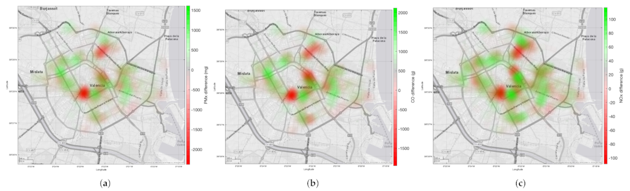
After obtaining $\alpha = 3.3$ as the best solution in terms of AQI, we will move on to analyze how the different pollutants are distributed throughout the city. We will compare this with respect to the default case. Figure 9 shows three different subfigures, one for each pollutant: PM${}_x$, CO, and NO${}_x$. Considering that green spots are areas where the amounts of pollutants are less than those in the default situation and that red spots represent the opposite, we observe that there is a reduction of pollutants along the target area, but there is an increase in other parts of the city. This could be because most of the vehicles are redirected to a route that traverses that area.

Figure 9. Difference in pollutants throughout the city with respect to the default case for $\alpha = 3.3$ (full traffic isolation). (a) PM${}_x$. (b) CO. (c) NO${}_x$.

Concerning the drawbacks of this solution, we found that, for the red area on the right side of Figure 9, the amount of pollutants increases by 46.34% on average. Specifically, the increase for each pollutant is: 48.98% for PM${}_x$, 50.65% for CO, and 39.39% for NO${}_x$. This was expected because most of the vehicles that traversed the old riverbed were deviated to this area. Since the AQI of the city did not increase and the amount of pollutants in the old riverbed decreased, the new distribution of the emissions is considered adequate.

Regarding the behavior of the traffic throughout the entire city, we obtained Table 3. In it, we can observe that, in terms of average speed, distance, and travel time for the different routes traversed by the different vehicles, the results remain similar. With respect to the volume of traffic along the old riverbed, Table 4 shows its behavior. As shown, the number of vehicles decreases by 15.55% compared to the default situation. Overall, we concluded that our restrictive solution not only improves pollutant emissions along the old riverbed, but it also achieves similar values for the average traffic flow parameters.

Table 3. Average traffic performance values in the city for the default and least-pollutant situations (full traffic isolation).

Metrics	Default Situation	$\alpha = 3.3$	$\Delta$ [%]
Speed	33.8 km/h	34 km/h	0.59
Distance	1206 m	1205 m	∼0
Time	189 s	188 s	−0.53

Table 4. Volume of traffic in the old riverbed for the default and least-pollutant situations (full traffic isolation).

Metrics	Default Situation	$\alpha = 3.3$	$\Delta$ [%]
N° of vehicles	6162	5204	−15.55

4.2. Partial Traffic Isolation

For this experiment, we will vary the $\alpha$ parameter again from 1 to 3.5 ($\alpha = 1$ is the default situation), but this time, restrictions will only be applied to streets near the old riverbed, but not to the bridges that cross it. By doing this, we will observe how emissions change for different $\alpha$ values and which one is the best for the target area.

Figure 10 shows the average percentage variation of pollutants for each $\alpha$ value with respect to the default case along the streets near the old riverbed. Specifically, three figures are shown (Figure 10a–c), one for each pollutant. For PM${}_x$, we notice that a major decrease takes place for $\alpha = 2.2;2.7$, with a difference of about 20%. Conversely, other $\alpha$ values, such as 1.6, increase the pollutant emissions by 15%. For CO, emissions decrease by almost 30% when $\alpha = 2.2$, and they increase by about 13% when $\alpha = 1.6$. NO${}_x$ emissions behave differently, as now, the best $\alpha$ is not 2.2, which increases by 7%, but rather $\alpha = 2.7;2.9$. Both have a decrease in emissions that is close to 7–8%.

Figure 10. Difference in pollutants with respect to the default case for various $\alpha$ values in the old riverbed (partial traffic isolation). (a) PM${}_x$. (b) CO. (c) NO${}_x$.

The percentage difference in emissions is not a complete way to determine the best solution. This is why we apply the ‘Fixed Box Model’ to calculate the AQI of the target area. To apply this model, we need to obtain the pollutant concentrations. Similarly to the experiment above, we will consider t = 1 h for NO${}_x$, t = 8 h for CO, and t = 24 h for PM${}_x$. Having said this, and assuming the conditions stated before, we obtained the different pollutant concentrations in the old riverbed for each $\alpha$ value (see Figure 11). Figure 11a shows the concentration of PM${}_x$, and, as shown, the lowest concentration is achieved when $\alpha = 2.2;2.7$. The same occurs for CO concentration (see Figure 11b), as for $\alpha = 2.2;2.7$, the lowest values are obtained, and $\alpha = 2.2$ is the lowest overall. NO${}_x$ is distributed differently, as the levels remain mostly the same, except for $\alpha = 1.1;1.4;2.3$, which break the trend.

Figure 11. Concentrations of pollutants in the old riverbed for each $\alpha$ value (partial traffic isolation). (a) PM${}_x$. (b) CO. (c) NO${}_x$.

Figure 12 shows the AQI of each pollutant for each $\alpha$ value. Figure 12a shows the different PM${}_x$ AQI values with respect to $\alpha$. As shown, the lowest value is achieved for $\alpha = 2.7$ with an AQI of 36. Regarding CO, and as can be seen in Figure 12b, the lowest value is hit by $\alpha = 3.2;3.3$ with an AQI of 55. The AQIs of NO${}_x$ are shown in Figure 12c, and, as we can observe, most of the $\alpha$ values have an AQI near 50, except for $\alpha = 1.1;1.4;1.7;1.8;2.1;2.5;3.5$, with an AQI of around 100. After analyzing the AQIs for each pollutant, we can determine the best general AQIs.

Figure 12. AQIs for each pollutant and $\alpha$ in the old riverbed (partial traffic isolation). (a) PM${}_x$. (b) CO. (c) NO${}_x$.

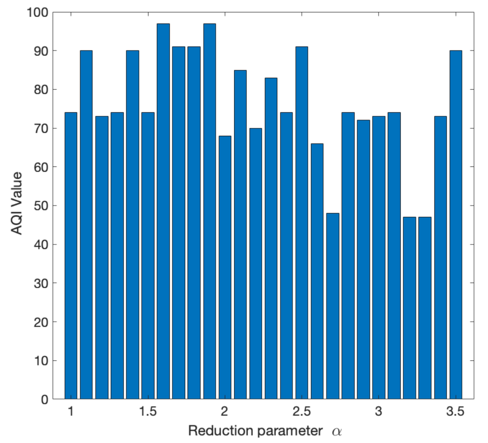
The global AQI for the old riverbed is shown in Figure 13. As we can observe, there are many values as results of the experiments. The best alphas ($\alpha = 2.7;3.2;3.3$) have an AQI value of 47–48, 25–26 points less than the default situation ($\alpha = 1$), which has an AQI of 73. The worst alphas ($\alpha = 1.6;1.9$) have an AQI of 97, with an increase of 24 with respect to the default case. In this way, we will now focus on the alphas with smaller amounts of pollutants in the old riverbed and try to figure out which one is the best. The solution with an alpha of 2.7 is selected. Focusing on how it performs in the city, we can conclude that $\alpha = 2.7$ has good results because it maintains the same amount of pollutants as the default approach, with an increase of merely 1.93%.

Figure 13. Global AQI in the old riverbed for each $\alpha$ (partial traffic isolation).

We will now focus on how the various pollutant emissions are distributed throughout the city when compared to the default situation (see Figure 14). Green spots are areas where the amounts of pollutants are smaller than those in the default situation. Red spots represent the opposite. Figure 14a shows the difference with respect to the default case for $\alpha = 2.7$ regarding the distribution of PM${}_x$ throughout the city. We observe that, in our target area, there is a decrease in emissions, but there is an increase in other parts of the city as well. The same occurs for CO (see Figure 14b) and NO${}_x$ (see Figure 14c). The red areas are the results of deviating traffic through those streets and, consequently, increasing pollutant emissions.

Figure 14. Difference in pollutants throughout the city with respect to the default case for $\alpha = 2.7$ (partial traffic isolation). (a) PM${}_x$. (b) CO. (c) NO${}_x$.

Every improvement also has its drawbacks, and for this solution, these are evidenced by the red areas that emerge. The average increase in pollutants for the big red area on the right of the map is 48.92%. Detailing the increase for each pollutant, we have that: For PM${}_x$, it is 44.24%; for CO, it is 54.01%; for NO${}_x$, it is 41.03%. This was expected, as most of the traffic is redirected to this area. Adding this to the previous results, we can observe that there is a redistribution of pollutant emissions. In general terms, the AQI for the city does not increase, since the increase in the red area is compensated by the decrease in our target area, as desired.

Finally, Table 5 shows the performance of the average traffic flow throughout the city for both the default and the least-pollutant situation. We observe that the speed of vehicles remains similar while travel time and distance increase by 1.59% and 0.58%, respectively, for the least-pollutant situation. Regarding the volume of traffic in the nearby streets of the old riverbed, the results are presented in Table 6. It shows that the number of vehicles decreases by 14.52%. In summary, for this method, we have a pollutant emission decrease in the target area and a negligible difference in average traffic flow data throughout the city.

Table 5. Average traffic performance values in the city for the default and least-pollutant situations (partial traffic isolation).

Metrics	Default Situation	$\alpha = 2.7$	$\Delta$ [%]
Speed	33.8 km/h	33.7 km/h	∼0
Distance	1206 m	1213 m	0.58
Time	189 s	192 s	1.59

Table 6. Volume of traffic in the old riverbed for the default and least-pollutant situations (partial traffic isolation).

Metrics	Default Situation	$\alpha = 2.7$	$\Delta$ [%]
N° of vehicles	6162	5267	−14.52

4.3. Comparison between Approaches

We will now compare the best results of the previous models ($\alpha = 3.3$ for full traffic isolation and $\alpha = 2.7$ for partial traffic isolation) in order to figure out which one is the best. Table 7 shows the different metrics analyzed and the differences between results.

Table 7. Comparison of metrics between the best $\alpha$ values of both approaches.

Metrics	Full Traffic Isolation $\mathit{\alpha } = 3.3$	Partial Traffic Isolation $\mathit{\alpha } = 2.7$	Difference
$\Delta$ PM${}_x$[%]	−7.75	−20.63	−12.88%
$\Delta$ CO [%]	−8.85	−23.21	−14.36%
$\Delta$ NO${}_x$[%]	−7.59	−7.37	0.22%
AQI	66	47	−19
N° of vehicles	5204	5267	1.21 %

On the one hand, by analyzing the variation in pollutants in the old riverbed with respect to the default case, we can notice that, in general, for $\alpha = 2.7$, the results are better, whereas for $\alpha = 3.3$, the amount of PM${}_x$ decreases by 7.75% with respect to the default situation, while for $\alpha = 2.7$, it decreases by 20.63%. The results for CO are even better, with a reduction of 23.21% with respect to the default case for $\alpha = 2.7$ and a difference of 14.36% for $\alpha = 3.3$. Contrarily, for NO${}_x$, both $\alpha$ values achieve similar results, with a decrease of about 7.5% with respect to the default case. Regarding the general AQI, for $\alpha = 2.7$, there is a reduction of 19 points with respect to the $\alpha = 3.3$ scenario. This is noticeable because, for partial traffic isolation, the AQI value is within the range of values considered to be “good”, while for the restrictive mode, it falls within the “moderate” range of values, as can be observed in Figure 3.

On the other hand, by examining the volume of traffic in the streets near the old riverbed, we can observe that the differences are negligible and mostly nonexistent.

The differences in the distribution of pollutants throughout the city between $\alpha = 3.3$ and $\alpha = 2.7$ can be seen in Figure 15. The green spots are for points where the amount of pollutants is smaller for the $\alpha = 2.7$ solution than for the $\alpha = 3.3$ solution. The red spots are the opposite. Considering this, we can observe that, in general, the amount of pollutants along the target area is reduced for the $\alpha = 2.7$ solution when adopting the partial traffic isolation. Specifically, regarding PM${}_x$ and NO${}_x$ (see Figure 15a,c), we can observe that there are more green spots, which is in accordance with the results obtained for the AQI.

Figure 15. Differences in pollutants with respect to $\alpha = 3.3$ (full traffic isolation) and $\alpha = 2.7$ (partial traffic isolation) throughout the city. (a) PM${}_x$. (b) CO. (c) NO${}_x$.

5. Conclusions and Future Work

In this paper, we have presented a solution to the urban pollution problem caused by traffic. Throughout this work, we intended to decrease the amounts of emissions near green areas by applying traffic constraints that minimize the traffic flow near those areas whenever possible.

We proposed two models to apply the restrictions—one with full traffic isolation and another with partial traffic isolation. For both, we analyzed the percentage difference with respect to the default situation in terms of the concentrations of pollutants in the studied area, the corresponding AQI value for the area, and traffic performance parameters.

The results show that, with partial traffic isolation, a better AQI is obtained in the old riverbed, with an improvement of 19 points, in addition to a reduction from a moderate to a good level according to the table of AQI levels. Similarly, the percentage difference in the amount of pollutants also has a better result when the partial traffic isolation model is adopted. The average decrease is 13.62% better than the full traffic isolation approach. At the same time, the traffic flow and pollution throughout the city remain mostly unaffected.

As future work, we intend to improve our algorithm. Our goal is to obtain a more complex equation for applying traffic restrictions. This means that our alpha value will not be enforced as the only parameter without dependence, but as a part of another equation that depends on the various pollutants, which will be weighted according to their impacts on health, i.e., 1 g of CO emitted is not the same as 1 g of PM${}_x$; therefore, this effect has to be accounted for in the chosen equation.

Finally, we also plan to continue studying the impacts of traffic restrictions for different situations—both to reduce pollution in an area and for other reasons (holidays, major events, etc.). In this sense, we want to apply a solution that is effective in the area that we focus on, as well as in the whole city.