Passenger Flow Prediction of Scenic Spot Using a GCN–RNN Model

Abstract

The prediction and control of passenger flow in scenic spots is very important to the traffic management and safety of scenic spots. This study aims to predict the passenger flow of a scenic spot based on the passenger flow of the bus and subway stations around the scenic spots. We propose a passenger flow prediction model based on graph convolutional network–recurrent neural network (GCN–RNN). First, a “graph” is constructed according to the geographical relationship between the scenic spot and the surrounding bus and subway stations. Then, characteristics of surrounding areas of bus and subway stations are constructed based on the crowd behavior analysis, and these are then used as the node-information of the “graph”. Last, the GCN–RNN model is used to extract the temporal and spatial characteristics of the passenger flow data of the scenic spot to realize the prediction. The experimental results show that the proposed model is effective in passenger flow prediction in scenic spots.

1. Introduction

A scenic spot is a place which often experiences a dense flow of people, and the passenger flow of a scenic spot refers to the number of tourists in the scenic spot at a specific time. With the acceleration of urbanization level in China, a large number of people have moved into cities, leading to continuous growth of the urban population [1]. High-density population agglomeration may cause major safety accidents. Therefore, accurately predicting the passenger flow of scenic spots is of great significance for preventing safety accidents in scenic spots. The prediction of passenger flow in scenic spots can provide an early warning of accidents, ensure the safety of the people, reduce economic losses, and play a very important role for decision makers and the public.

At present, the research methods of passenger flow prediction in scenic spots can be divided into two categories. The first type is the traditional prediction methods of passenger flow in scenic spot, which mainly include wavelet analysis [2], EMD [3], the use of regression analysis [4], grey model [5], wavelet transform, LS-SVM [6], probability tree [7], wavelet-SVM [8], Markov, and other methods [9,10]. Another type of prediction methods is based on deep learning. At present, more scholars use deep learning methods to predict passenger flow in scenic spots, including LSTM [11], improved BP neural network optimized by genetic algorithm [12], improved BP neural network optimized by particle swarm optimization [13], generalized deep belief network particle swarm optimization prediction model [14], stacked autoencoders with deep neural networks [15], and adaptive networks [16], etc.

Through the study of the two prediction methods, the traditional prediction methods [2,3,4,5,6,7,8,9] based on specific mathematical models have strong theoretical support and are easy to understand, but their adaptability to data is poor. For example, ARIMA model [9] is more suitable for stationary data, such as house price prediction. However, it does not work well for predicting non-stationary data, such as stock market prediction. Even if there is a combination of traditional prediction methods, its application range is far inferior to deep learning prediction methods. The deep learning prediction methods based on a big data background can realize data analysis in high-dimensional space, and the structure of the deep learning model is highly variable, which makes the application range of this method more extensive. Therefore, we choose the deep learning method to study the passenger flow prediction of scenic spots.

However, the current deep learning models lack the temporal and spatial characteristics of scenic spot data, and do not conduct a comprehensive analysis of scenic spot data. Spatial information refers to the passenger flow of the bus and subway stations around the scenic spot, and whether there are areas near the scenic spots, such as schools and residential areas, etc. This information may have an impact on the prediction of passenger flow in the scenic spots, and GCN can extract the features of the topological structure data, where the graph is composed of nodes and edges.

Therefore, we use GCN to extract spatial location information in this paper. According to the relative geographical position of the scenic spot passenger flow data, the ‘graph’ is constructed, and the node-information is constructed according to the crowd behavior analysis. The passenger flow prediction of scenic spots is essentially a time series problem, so we use RNN to extract time dimension information. Combining these two models, a GCN–RNN scenic spot passenger flow prediction model is formed, which is used to extract the temporal and spatial characteristics of the scenic spots.

In this paper, we make the following contributions:

(1)

Considering the spatial location characteristics of the scenic spot, a graph structure is constructed according to the geographic location of the scenic spot and the surrounding bus and subway stations. Features are extracted through the graph convolution network. Moreover, considering the daily behavior of the crowd, the features of the surrounding area of the scenic spot are used as the node information to assist the model prediction.

(2)

A new model GCN–RNN for passenger flow prediction in scenic spots is proposed. In addition to extracting spatial features with graph convolution, recurrent neural networks are also used to extract temporal features.

(3)

The method in this paper is compared with several state-of-the-art methods to demonstrate its effectiveness. It is also necessary to verify the effectiveness of the graph convolutional network and surrounding area features. The surrounding features of the scenic spots play a positive role in the prediction as auxiliary information.

The rest of this paper is arranged as follows. Section 2 provides a review of related work. Section 3 introduces the proposed method of passenger flow prediction in scenic spots. In Section 4, the experiments of passenger flow prediction of the South Luogu Lane scenic spot in Beijing are presented. The comparison results of different models are provided. Section 5 discusses the methods and limitations of this paper. Finally, Section 6 summarizes this paper and highlights future research suggestions.

2. Related Work

2.1. Prediction Methods of Scenic Spot Passenger Flow

2.1.1. Machine Learning and Statistical-Based Methods

In 2011, Zhao et al. [2] used wavelet analysis to decompose passenger flow data at multiple scales, and then used a neural network to predict the sequence. In 2012, Yu et al. [3] predicted the passenger flow of Huangshan Scenic Spot based on the fluctuation characteristics of EMD. In 2013, Cui et al. [4] used regression analysis and grey model to predict the visitor flow of Shiyuan. Yang et al. [5] predicted large passenger flow based on the grey Markov model. Based on the historical OD passenger flow data of various large-scale activities, the grey model is established for the passenger flow data by using the grey prediction algorithm, and then the Markov correction model is established. Finally, the prediction error is used to correct the gray prediction result to produce the final predicted large passenger flow value. Yang et al. [6] conducted real-time passenger flow prediction based on discrete one-dimensional Daub4 wavelet analysis and least squares support vector machine (LS-SVM). LS-SVM is used to predict the low-frequency and high-frequency components of passenger flow time series data, and the wavelet analysis method reconstructs the predicted low-frequency and high-frequency components. Leng et al. [7] proposed a passenger flow model based on a probability tree. In 2015, Sun et al. [8] proposed a novel passenger flow prediction model of wavelet-SVM short-time. In 2018, Yan et al. [9] used an autoregressive integrated moving average model to predict the short-term traffic flow of the subway. The authors selected the most appropriate parameters through stationarity testing, model identification, parameter estimation, and model diagnosis and prediction. In 2020, Zhang et al. [10] proposed a passenger flow prediction method based on ST-LightGBM.

2.1.2. Deep Learning-Based Models

In 2011, Li et al. [11] predicted the passenger flow of scenic spots based on a long-term and short-term memory network. In 2014, Song et al. [12] predicted the daily passenger flow based on a BP neural network optimized by improved the genetic algorithm. In 2015, Yu et al. [13] proposed an improved particle swarm optimization BP neural network for tourist flow prediction. In 2017, Zhao et al. [14] proposed the generalized deep belief network particle swarm optimization prediction model and applied it to the scenic spot passenger flow prediction. Liu et al. [15] combined stacked autoencoders with deep neural networks. The temporal features were combined with scene features such as entry and exit, and ticket cards, etc., and the deep neural network was further initialized through the pre-trained stacked autoencoder. Li et al. [16] proposed an adaptive network. Pekel et al. [17] developed two hybrid methods, namely parliamentary optimization algorithm–artificial neural network (POA–ANN), and intelligent water drops algorithm–ANN. In 2019, Shiva et al. [18] used an adaptive network to predict passenger flow. Liu et al. [19] proposed a deep passenger flow model. The model is an end-to-end deep learning architecture that is highly flexible and scalable, achieving high prediction accuracy. Li et al. [20] proposed a dynamic radial basis function neural network, which can identify key sites and time periods 30 min in advance. In 2021, Gao et al. [21] proposed an attention-based subway spatio-temporal convolution model (AMSTCN) for short-term passenger flow prediction.

The recent passenger flow prediction methods for scenic spots are based on deep learning models, but the current methods rarely consider the impact of spatial information around scenic spots on passenger flow. Therefore, this paper introduces a graph convolutional network to extract the spatial location features around the scenic spot.

2.2. Graph Convolutional Network

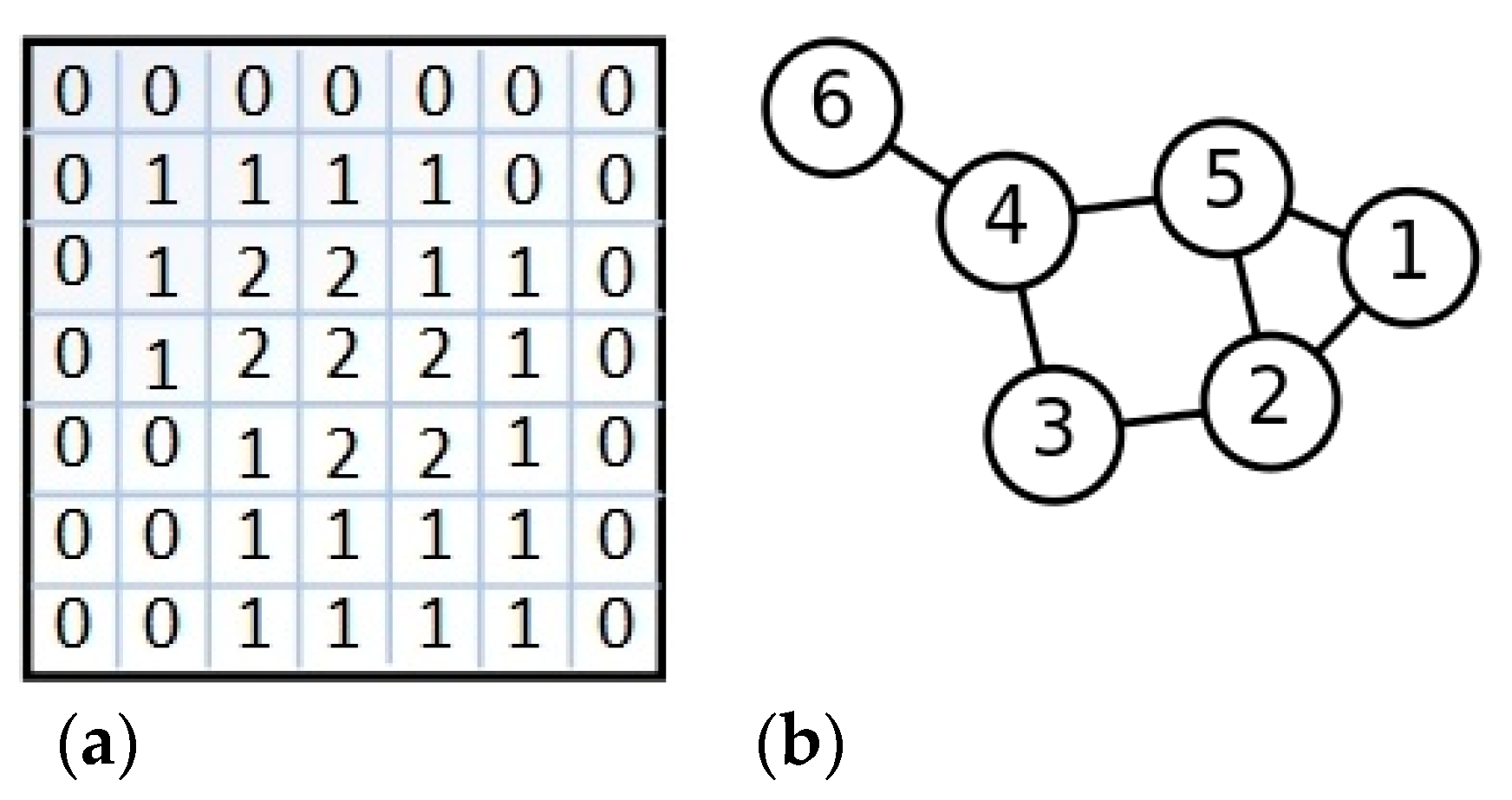
For standard matrix data, such as images, we can use the convolutional neural network (CNN) to extract their features. The data processed by CNN are in the form of a matrix, which is based on a matrix arranged by pixels. This form of data is called the Euclidean structure, as shown in Figure 1a. However, there are a lot of non-standard forms of data in our daily life, and the ‘topology structure’ (‘graph’) is one of them. Topological graphs in the computer field are different from images in the usual sense [22]. Topological graphs are generally composed of points and edges, which are collectively referred to as a ‘graph’. The ‘Graph’ diagram is as shown in Figure 1b. The numbers represent the points in the ‘graph’, and the lines connecting the points are the edges. For this type of data, it cannot be extracted with the convolutional neural network. Therefore, a graph convolutional network (GCN) is proposed.

The graph convolution network has been successfully applied in many fields. For example, in the prediction of chemical reactivity through graph convolutional networks [23], prediction of grasp stability with tactile sensors [24], for action recognition [25], and for semi-supervised classification [26,27], etc. Moreover, graph convolutions come in many different variants, topology adaptive graph convolutional networks [28], and a convolutional neural network over large-scale labeled graphs [29]. The graph convolutional network is proposed based on the spectral convolution network. Spectrum convolution [30,31] is different from CNN, in that the convolution kernel is fourier transformed [32], and the expression is as follows:

$$g(\theta )\times x=Ug(\theta )U^{T}x$$

(1)

where $U$ is the eigenvector matrix of normalized Laplace operator, $U^{T}x$ is the transform of convolution kernel $x$ in Fourier domain.

$$L=I_N-D^{-\frac{1}{2}}A{D}^{-\frac{1}{2}}=U\Lambda U^T$$

(2)

Equation (2) is Laplace operator, $I_N$ is the identity matrix, $\Lambda$ is the characteristic diagonal matrix of eigenvalues. In the spectrum calculation, $g(\theta )$ is regarded as the function $g_{{\theta }^{\prime }}(\Lambda )$ of $L$ eigenvalue. Due to the huge amount of computation, Hammond proposed to use k-order Chebyshev polynomials in 2011, the expression is as follows:

$$g_{{\theta }^{\prime }}(\Lambda )\approx {\displaystyle \sum _{k=0}^K{{\theta }^{\prime }}_k}{T}_k(\tilde{\Lambda })$$

(3)

where ${{\theta }^{\prime }}_k$ is the coefficient of Chebyshev polynomial and $T_k(\tilde{\Lambda })$ is Chebyshev polynomial, by introducing the above formula into (1), we can produce the following results:

$$g_{\theta }{}^{\prime }\times x\approx {\displaystyle \sum _{k=0}^K{\theta }_k{}^{\prime }{T}_k}(\tilde{L})x$$

(4)

If K is set to 1, the (4) type can be expanded to:

$$g_{\theta }{}^{\prime }\ast x={\theta }_0{}^{\prime }x+{\theta }_1{}^{\prime }(L-I_N)x={\theta }_0{}^{\prime }x+{\theta }_1{}^{\prime }{D}^{-\frac{1}{2}}A{D}^{-\frac{1}{2}}x$$

(5)

where ${\theta }_0{}^{\prime }$ and ${\theta }_1{}^{\prime }$ are parameters, and (5) is reduced to:

$${g^{\prime }}_{\theta }=\theta (I_N+D^{\frac{1}{2}}A{D}^{\frac{1}{2}})x$$

(6)

$I_N+D^{\frac{1}{2}}A{D}^{\frac{1}{2}}$ fixed the eigenvalue between (0,2), as the number of iterations increases, the gradients disappear and explode gradually. In order to solve this problem, the above parameters are normalized:

$$g_{\theta }\times x=\theta {\tilde{D}}^{-\frac{1}{2}}\tilde{A}{\tilde{D}}^{-\frac{1}{2}}x$$

(7)

where $\tilde{A}=I_N+A$, ${\tilde{D}}_{ii}={\displaystyle \sum _j{\tilde{A}}_{ij}}$, extend the model to the high-dimensional vector data to obtain:

$$Z={\tilde{D}}^{-\frac{1}{2}}\tilde{A}{\tilde{D}}^{-\frac{1}{2}}X\theta$$

(8)

$\theta \in R^{C\times F}$ is the convolution parameter, $X\in R^{N\times C}$ is the input of the model, and $Z\in R^{N\times F}$ is the convoluted matrix.

This paper is dedicated to solving the problem of passenger flow prediction in scenic spots, not only considering the temporal features, but also the spatial features around the scenic spot. Such spatial features can be structured as topological structures, which can only be extracted by the graph convolution network. Therefore, the graph convolutional network plays a crucial role in our model.

3. Methods

The South Luogu Lane is one of the oldest neighborhoods in Beijing, China. It is located in the Jiaodaokou area on the east side of Beijing’s central axis, in the center of Beijing. It is a chessboard-style traditional residential area with the largest scale, the highest grade, and the most abundant resources in our country, which completely preserve the Hutong courtyards of the Yuan Dynasty. Today, it is a famous scenic spot in Beijing, with great tourism value, attracting tourists from all over the world [33]. According to statistics, the average daily passenger flow of the South Luogu Lane exceeds 30,000, the weekend passenger flow exceeds 50,000, and the holiday passenger flow exceeds 100,000. All seasons are suitable for tourism, so the difference in passenger flow between different seasons is not particularly large. Moreover, the surrounding traffic is convenient, with many subway lines and bus stops. Therefore, this paper takes the South Luogu Lane scenic spot as an example to predict the passenger flow of the scenic spot.

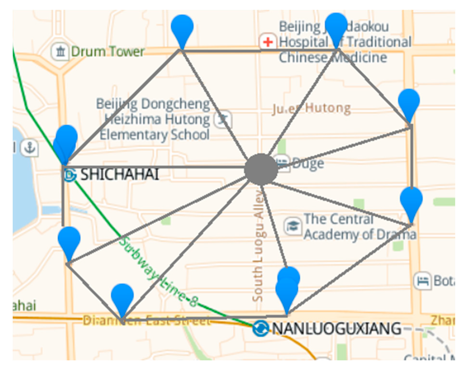
To construct graph convolution, we first construct the ‘graph’ of the scenic spots and the stations, as shown in Figure 2. (The figure is taken from a real map.) The gray circle in the figure is the center of the South Luogu Lane scenic area, and the blue signs are the bus and subway stations around the scenic spot. Visualize the geographical location of the South Luogu Lane scenic spot and the surrounding bus and subway stations to form a topological graph.

There is road connection between the scenic spot and the stations, so the passenger flow between the scenic spot and the stations can flow freely. For example, passengers who disembark at the South Luogu Lane bus station may walk to the South Luogu Lane subway station and board a bus to leave. However, some passengers who disembark from the station may not go to the scenic spot, but go to other places around the scenic spot. Therefore, it is also necessary to consider the characteristics and attributes of the area around the scenic spot, which will affect the passenger flow of the scenic spot. In addition, the passenger flow between stations also influences each other, so these mutually influencing nodes can be connected by edges to form a topology graph, and then features are extracted through a graph convolutional network.

Therefore, we propose a graph convolutional network–recurrent neural network (GCN–RNN) model to predict the passenger flow in the scenic spots by extracting the spatial–temporal characteristics of the scenic spots and surrounding stations. The input of the model is a ‘graph’, and the adjacency matrix is the connection of roads. The node-information is passenger flow data and surrounding area features, as is shown in Figure 3.

3.1. Construction of “GRAPH” According to Scenic Spots

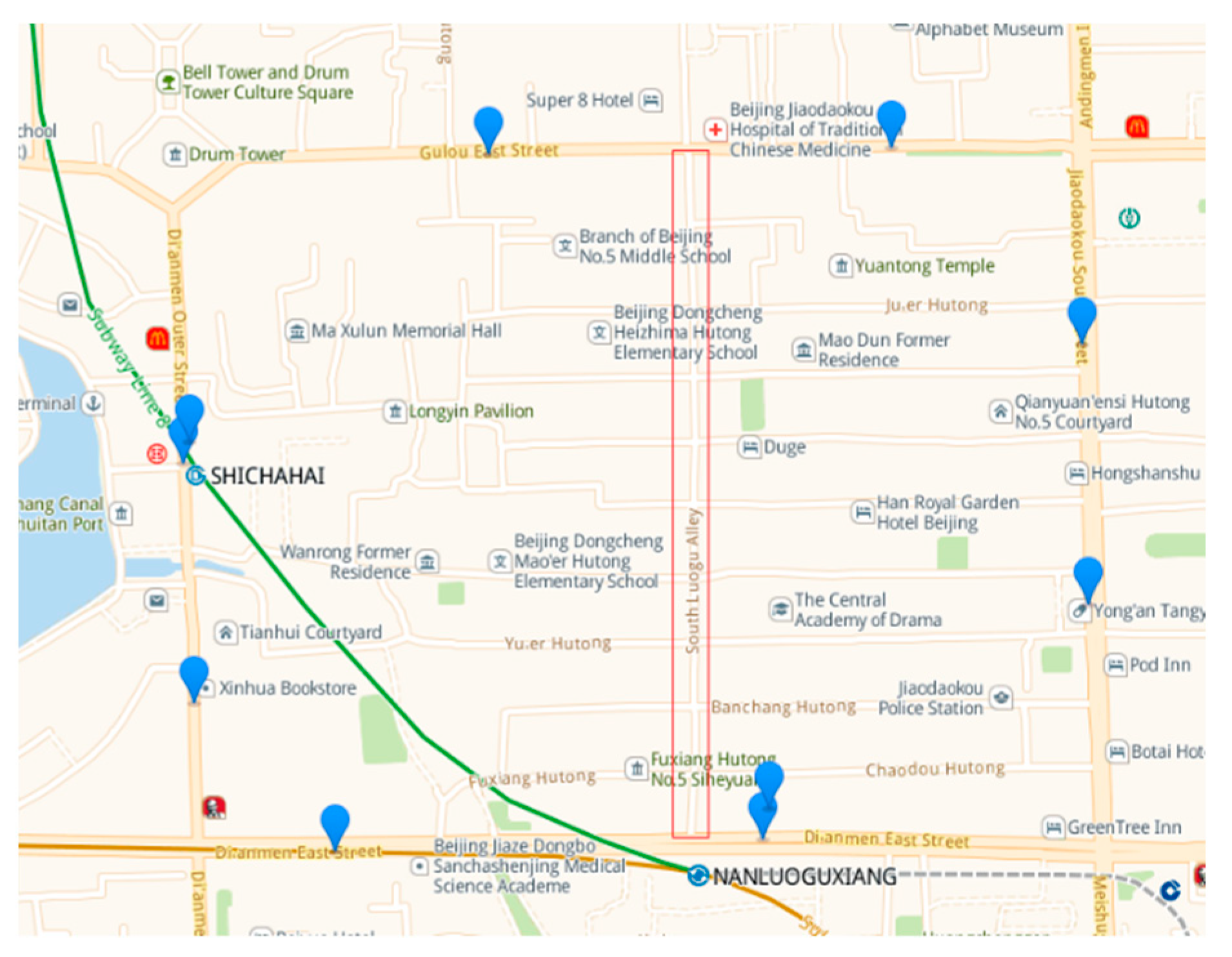
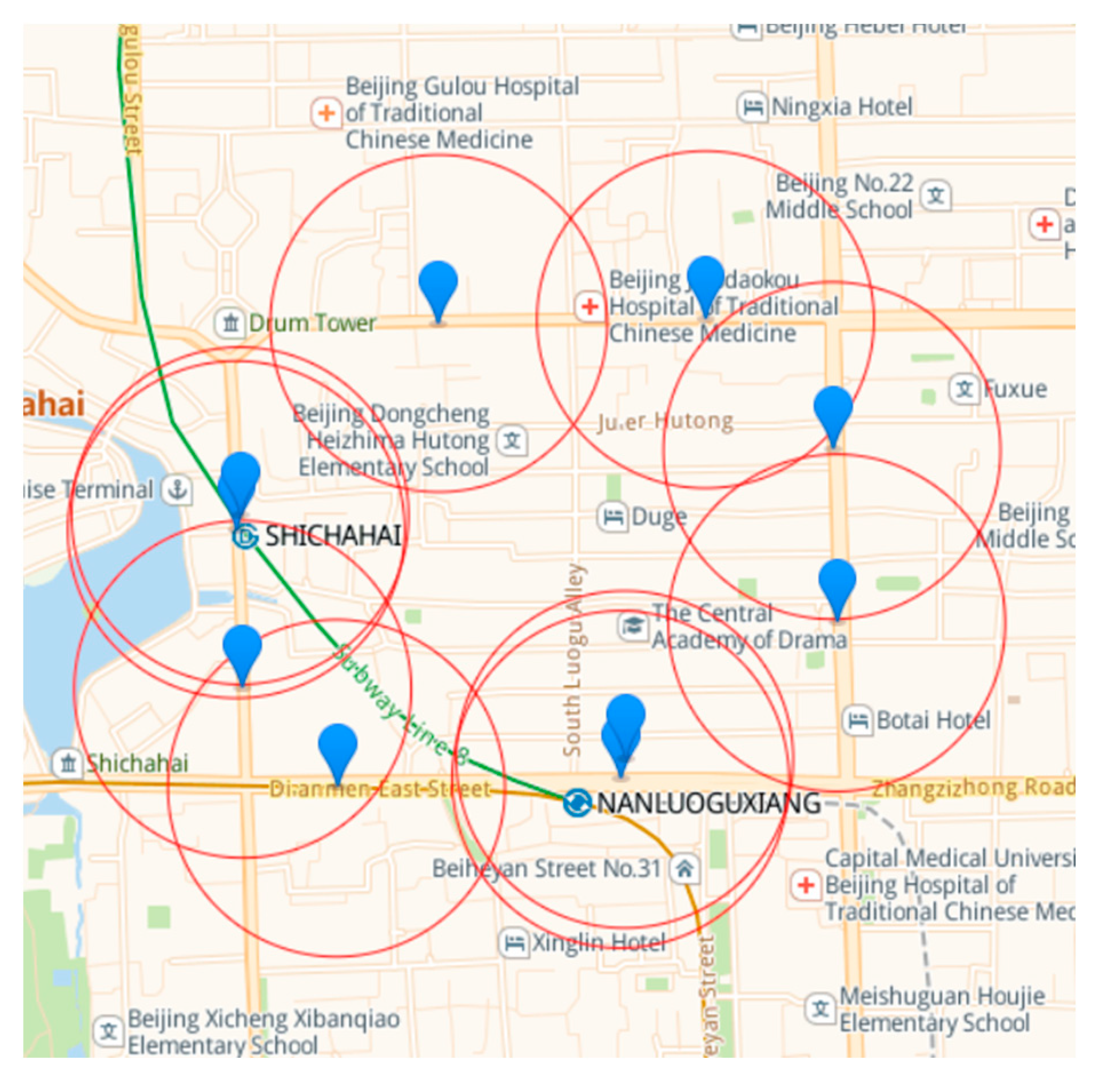
Figure 4 shows the geographical–location relationship between the South Luogu Lane scenic spot and the surrounding 10 bus and subway stations. The red dots indicate subway stations, and the blue dots indicate bus stations. The South Luogu Lane scenic spot is a road in the middle (the red area above). It is obvious that the relationship between the stations and the scenic spot constitutes a ‘graph’ structure. There are 11 nodes in the ‘graph’, which are composed of bus, subway stations, and the South Luogu Lane scenic spot. Moreover, there are different areas around the station. According to the analysis of crowd behavior, these areas may affect the passenger flow at the station. As shown in Figure 5, if passengers disembark at the South Luogu Lane bus stop, they may also go to the Weaving and Dyeing Bureau Primary School, Beijing Hospital of Traditional Chinese Medicine, or the Central Academy of Drama, etc.

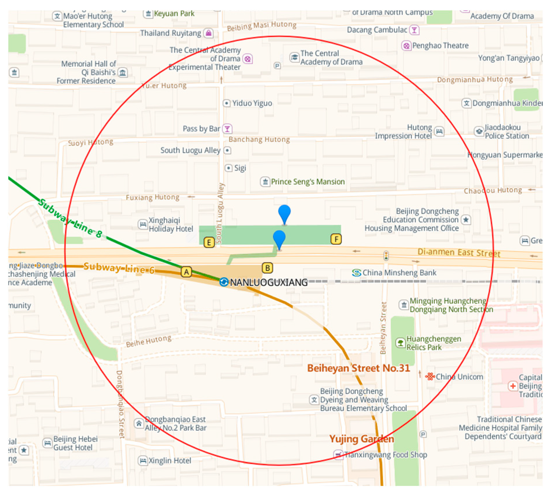
Based on the above analysis, we think that the existence of “school”, “residential areas”, “business districts”, and “other scenic spots” in the surrounding areas will affect the passenger flow of the stations. Consequently, this paper defines the characteristics of surrounding areas (CSA) within 500 m around the station (as shown in Figure 6). The specific method is to judge whether there are “schools”, “residential areas”, “business districts”, and “other scenic spots” in the area. If there is the above area, it is recorded as 1, if not, it is recorded as 0 (the CSA of the South Luogu Lane scenic spot is recorded as (1,1,1,1)). As a result, the node characteristic information of the graph is represented by (passenger flow, CSA). The adjacency matrix of the graph is constructed based on the geographical relationship between the nodes and whether there are direct road connections.

3.2. GCN–RNN Model

The spatial location information and time dimension information are equally important in the passenger flow prediction of the South Luogu Lane scenic spot. Therefore, we propose a GCN–RNN scenic spot passenger flow prediction model, which extracts spatial location information by GCN and temporal dimension information by RNN. The GCN–RNN model consists of a two-layer graph convolutional network and a layer of recurrent neural network. The model architecture is shown in Figure 3.

The two-layer GCN is used to fuse the direct and indirect related information of the node. This should not only consider the relationship between the station and the scenic spot, but also the interaction between the stations. The model expression is as follows:

$$y_1,y_2,\cdots ,y_N=f(g_1,g_2,\cdots ,g_N)$$

(9)

where N is the prediction stride, the graph (g) is the input, and the vector $y\in R^{1\times N}$ is the final output prediction value, which is the passenger flow of the scenic spot to be predicted.

3.3. Training Algorithm

This paper is based on python3.6 to train the model, the computing environment is torch 1.6.0 + CPU and DGL 0.5.2. The number of iterations is 2500. The training time of the model is 1617.29 s, and its pseudo-code flow is as follows:

Training steps

Input: training set $D={\left\{\left(x_k\right)\right\}}_{k=1}^m$

Learning rate 1e-2  Evaluation index L1_loss  Optimizer Adam

Process: Initialize GCN and RNN model  for all $(x_k)\in D$ do: Build a ‘graph’, in which features include the site passenger flow and the characteristics of the area around the site. Input $g_1,g_2,\cdots ,g_t$ to GCN network, and output $h_1,h_2,\cdots ,h_t$ (t represents time). Input $h_1,h_2,\cdots ,h_t$ to RNN network, and output $y_1,y_2,\cdots ,y_t$. Output: model predicted values $y_1,y_2,\cdots ,y_n$.

4. Experiments and Results

4.1. Data

The data used in this paper include the passenger flow data of the South Luogu Lane scenic spot and 10 bus and subway stations surrounding it. The dataset is composed of 15-min granular passenger flow data from November 2018 to November 2019 at 8:00–22:00 every day.

Table 1. Some examples of raw data. “In” represents the number of arrivals at the site, “Out” represents the number of people leaving the site, “lgx” represents Luoguxiang Station, “jdkn” represents Jiaodaokou South Station, “bbms” represents Beibing Masi Station, and “dhcgbk” represents Donghuangcheng Genbeikou Station.

DateTime	lgxIn	jdknOut	jdknIn	bbmsOut	bbmsIn	dhcgbkOut	dhcgbkIn
1 November 2018 8:00	8	30	25	15	16	13	5
1 November 2018 8:15	20	31	45	33	35	16	2
1 November 2018 8:30	23	33	51	22	25	8	1
1 November 2018 8:45	25	52	59	14	27	16	5
1 November 2018 9:00	26	33	99	5	23	8	0
1 November 2018 9:15	23	29	69	4	13	12	2
1 November 2018 9:30	12	41	58	16	20	19	1
1 November 2018 9:45	26	72	101	16	25	11	2
1 November 2018 10:00	11	22	51	10	20	14	4
1 November 2018 0:15	16	90	97	11	37	11	9
1 November 2018 10:30	23	24	46	19	32	4	0
1 November 2018 10:45	16	43	57	14	17	10	0
1 November 2018 11:00	13	31	56	14	49	11	4
1 November 2018 11:15	17	44	68	23	14	12	1
1 November 2018 11:30	4	78	68	21	26	7	1
1 November 2018 11:45	18	27	50	26	27	19	1
1 November 2018 12:00	26	35	60	13	14	6	2

is part of the raw data. (The complete data are not allowed to be public.) The first 80% of the dataset is the training set, and the last 20% is the test set. The evaluation indexes are least absolute error (LAE) and mean absolute percentage error (MAPE), as show in Formula (10) and (11).

$$LAE(y,\widehat{y})={\displaystyle \sum _{i=0}^m|y^i}-{\widehat{y}}^i|$$

(10)

$$MAPE=\frac{1}{m}{\displaystyle \sum _{i=0}^m\frac{|y^i-{\widehat{y}}^i|}{{\widehat{y}}^i}}\times 100$$

(11)

where $y_i$ is the predicted value and ${\hat{y}}_i$ is the ground truth.

4.2. Results

We compare the model proposed in this paper with the time series models RNN and LSTM used for passenger flow prediction in scenic spots. For the training of the model RNN and LSTM, the equipment and parameters used are consistent with the method proposed in this paper. The evaluation indicators are L1 loss and mean square error. The smaller the value of L1 loss (LAE) and mean square error (MAE), the better the performance of the algorithm. As shown in

Table 2. Model error comparison.

Method	LAE 1	MAPE 2 (%)
RNN	42.40	22.87
LSTM	43.72	48.01
FCN–RNN	35.53	19.47
GCN–RNN (w/o CSA)	21.50	10.94
GCN–RNN	6.57	3.20

¹ Least absolute error. ² Mean absolute percentage error.

, the LAE of RNN is 42.4, and the mean square error is 22.87%. The LAE of LSTM is 43.72, and the mean squared error is 48.01%. The LAE and mean squared error obtained by the model proposed in this paper are 6.57% and 3.2%, respectively. Therefore, the performance of the model proposed in this paper in predicting the passenger flow of scenic spots is better than the above methods.

In addition, we replace the GCN in the model of this paper with FCN to compare the performance. FCN–RNN refers to a model that uses a fully connected network instead of a graph convolutional neural network. The mean squared error of FCN–RNN is 19.47%. It can be seen that the error obtained by replacing the GCN model is larger, so it is verified that the graph convolutional network is better for extracting spatial features. To demonstrate the effectiveness of surrounding area features, we retrain the GCN–RNN model without characteristics of the surrounding area (w/o CSA), and the mean squared error is 10.94%. It is evident that the model without CSA performs poorly.

Figure 7 more intuitively shows the performance comparison between the method in this paper and the popular passenger flow prediction algorithms in scenic spots. The green line in the figure is the L1 loss of the model, and the blue line is the mean squared error of the model. The GCN–RNN model performs best under the two evaluation indexes. It further proves that the method proposed in this paper is more effective in predicting tourist flow in scenic spots compared to RNN and LSTM. Moreover, the GCN model is better than FCN in extracting the spatial characteristics of passenger flow data in scenic spots, which proves the influence of CSA on passenger flow in scenic spots.

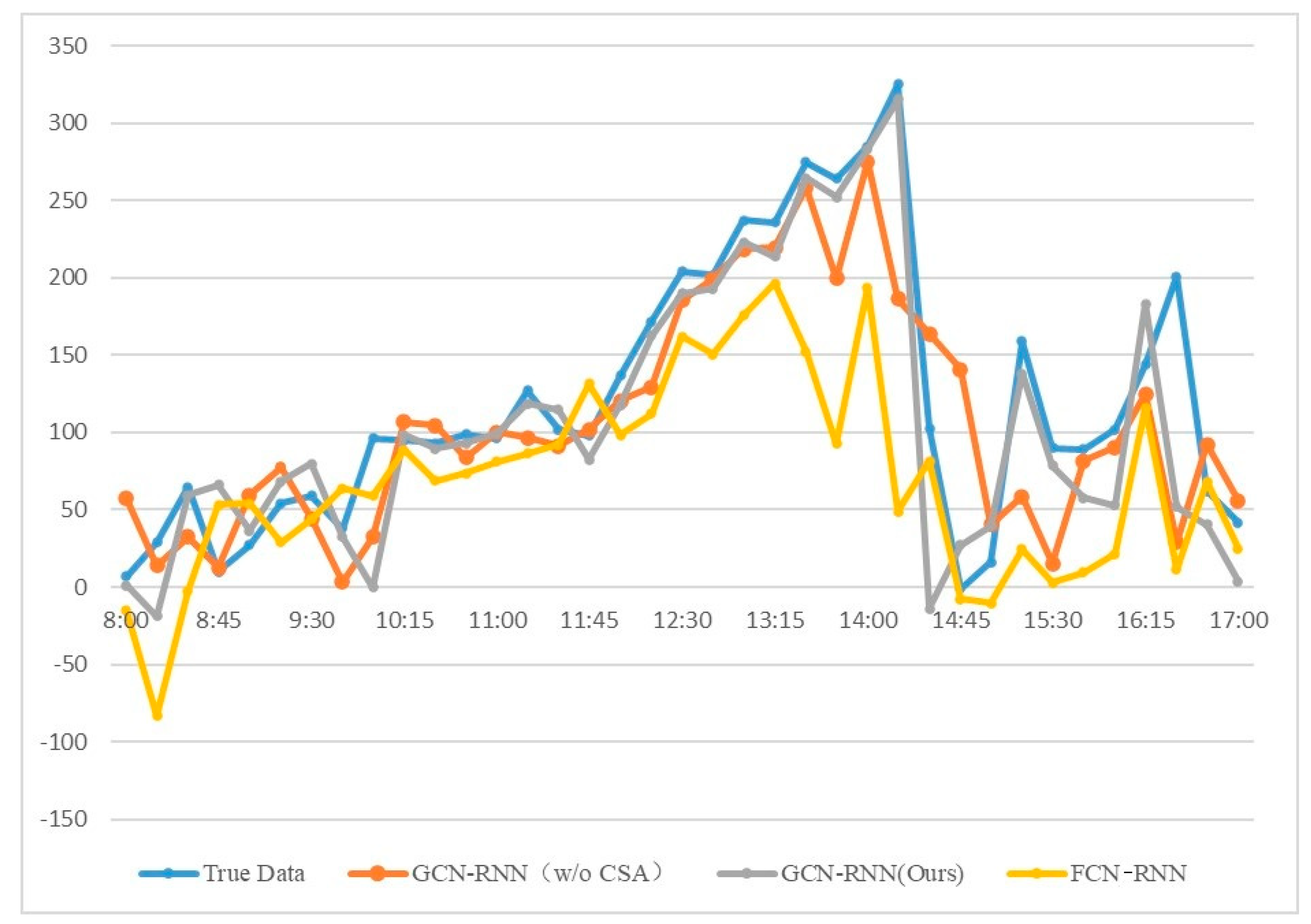
In order to observe the fluctuations of passenger flow prediction in scenic spots more clearly, we draw the real data curves and the predicted fluctuation curves of the GCN–RNN model and two other models, including GCN–RNN (w/o CSA) and FCN–RNN model. As shown in Figure 8, the horizontal coordinate is the time (the time period from 8:00 to 17:00 is selected, and the time interval of the data is 15 min), and the vertical coordinate is the fluctuation of the number of tourists in the scenic spot. The blue line is the fluctuation of the real data, and the orange line is the predicted passenger flow of the scenic spot by GCN–RNN, which does not use the surrounding area features (w/o CSA). The yellow line is the passenger flow predicted by the FCN–RNN model that replaces the graph convolution with the fully connected layer, and the gray line is the tourist flow predicted by our proposed GCN–RNN model. Obviously, the predicted value curve (gray) obtained by our GCN–RNN model is the closest to the true value curve (blue). GCN–RNN (w/o CSA) (orange) is followed, and FCN–RNN (yellow) is the worst.

Compared with the FCN–RNN model, the trend of GCN–RNN prediction curve is consistent in most time periods, such as 12:30–13:00, 13:15–14:00, 16:15–16:45, and so on. However, the FCN–RNN model is quite different from the GCN–RNN model, indicating that the FCN model has a weaker ability in spatial feature extraction. Compared with the GCN–RNN (excluding CSA) model, the GCN–RNN (excluding CSA) model also has some deviation from the GCN–RNN model, but the deviation is smaller than the FCN–RNN model. It is proved that CSA, as auxiliary information, plays an active role in the prediction.

5. Discussion and Limitations

By studying the passenger flow of the South Luogu Lane scenic spot in the center of Beijing, a GCN–RNN based scenic spot passenger flow prediction model is proposed. The model can be widely used in passenger flow prediction of other scenic spots. Compared with the traditional scenic spot passenger flow prediction method, it is obvious that the deep learning algorithm adopted in this paper is faster and has stronger performance. There is no doubt that the model proposed in this paper is effective for scenic spot passenger flow prediction and outperforms current deep learning models in terms of performance because it achieves the lowest mean square error. Different from the current deep learning models, the model in this paper considers both temporal and spatial features, so it achieves better results.

For holidays and weekdays, the passenger flow of scenic spots is quite different, which may affect the forecast of passenger flow. Therefore, in future research, we will further conduct cluster analysis on the data of holidays and working days, and then use convolutional neural networks to extract features, and add these features to the GCN–RNN model to assist prediction.

6. Conclusions

With the continuous development of tourism, a large number of people may go to scenic spots, and large-scale gatherings may lead to safety accidents, so it is necessary to predict the passenger flow of scenic spots. At present, the more popular deep learning-based methods pay less attention to the influence of spatial characteristics of scenic spots on passenger flow. Moreover, almost no consideration is given to the regional characteristics around the scenic spot.

The research contributions of this paper are as follows: we successfully introduce a graph convolutional network to extract the spatial location features of scenic spots and surrounding geographic information. Based on the real geographic data and analysis of crowd behavior, the characteristics of the surrounding area are used as the node-information to assist the model for prediction. RNN is used to extract the temporal characteristics of passenger flow in scenic spots. A new model GCN–RNN for scenic spot passenger flow prediction is proposed. The model consists of two layers of graph convolution network and one layer of recurrent neural network. Our method comprehensively considers the spatiotemporal characteristics of scenic spot data, and analyzes the possible impact of schools and residential areas around the scenic spot on the passenger flow of the scenic spot. Experiments show that our method can effectively predict the passenger flow of scenic spots.

In the experiment, we compared GCN–RNN model with LSTM and RNN, which are classic time series models. The evaluation indicators are L1 loss and mean square error. The experimental results show that the method proposed in this paper performs best under the two evaluation indicators, which proves the effectiveness of the model. In addition, we also verified the effectiveness of the graph convolution network, replacing the graph convolution in the GCN–RNN model with a fully connected network. The mean square error obtained by the replaced model is significantly higher than that of the model in this paper. This also shows that compared with fully connected network, GCN can extract spatial features better. For data with graph structure, GCN can be used to extract features. Furthermore, our model is not only suitable for passenger flow prediction in the South Luogu Lane scenic spot, but can also be applied to any other scenic spot for passenger flow prediction. The proposed model is of great significance for the prediction of passenger flow in scenic spots.

According to our experiments, the changing trend of passenger flow in scenic spots is complex, and there are many factors that affect the change of passenger flow. In future research, in addition to exploring the characteristics of time and space dimensions, the passenger flow in scenic spots will also be predicted based on the crowd behavior dimension. Our analysis is mainly aimed at the passenger flow of bus stations and subway stations around the scenic spot, but the transportation methods are not limited to the above two, and may also include taxis, bicycles, and other transportation methods. Therefore, we will further consider the passenger flow of various transportation modes in the future, continue to improve the model, and then better predict the passenger flow of scenic spots.

References

- Zhu, N.; Zeng, Z.J. Analysis of the determinants of urban population growth in China. China Popul. Sci. 2004, 5, 9–18. [Google Scholar]
- Zhao, S.Z.; Ni, T.H.; Wang, Y. A new approach to the prediction of passenger flow in a transit system. Comput. Math. Appl. 2011, 61, 1968–1974. [Google Scholar] [CrossRef] [Green Version]
- Yu, X.Y.; Sha, R.; Zhu, G.X. EMD Based passenger flow fluctuation characteristics and its combination prediction in scenic spots—A case study of Huangshan Scenic Spot. Adv. Earth Sci. 2012, 31, 1353–1359. [Google Scholar]
- Cui, L.M. Research on the Forecast and Early Warning of the World Garden Visitors Flow Based on the Network Search Behavior; Qingdao University of Technology: Qingdao, China, 2013. [Google Scholar]
- Yang, J.; Hou, Z.S. A real time forecasting model of large passenger flow based on Grey Markov. J. Beijing Jiaotong Univ. 2013, 2, 119–123. [Google Scholar]
- Yang, J.; Hou, Z. A Wavelet Analysis Based LS-SVM Rail Transit Passenger Flow Prediction Method. China Railw. Sci. 2013, 34, 122–127. [Google Scholar]
- Leng, B.; Zing, J.B.; Xiong, Z. Probability tree based passenger flow prediction and its application to the Beijing subway system. Front. Comput. Sci. 2013, 7, 195–203. [Google Scholar] [CrossRef]
- Sun, Y.X.; Leng, B.; Guan, W. A novel wavelet-SVM short-time passenger flow prediction in Beijing subway system. Neurocomputing 2015, 166, 109–121. [Google Scholar] [CrossRef]
- Yan, D.; Zhou, J.; Zhao, Y.; Wu, B. Short-Term Subway Passenger Flow Prediction Based on ARIMA. In Proceedings of the International Conference on Geo-Spatial Knowledge and Intelligence 2018, Wuhan, China, 14–16 December 2018. [Google Scholar]
- Zhang, Z.; Wang, C.; Gao, Y. Short-Term Passenger Flow Forecast of Rail Transit Station Based on MIC Feature Selection and ST-LightGBM considering Transfer Passenger Flow. Sci. Program. 2020, 2020, 3180628. [Google Scholar] [CrossRef]
- Li, J.; Wei, Z.J.; Wang, S.; Chen, L.J. Short-term passenger flow prediction of subway stations based on deep learning Long and Short-term Memory network structure. Urban Mass Trans. 2011, 21, 49–53. [Google Scholar]
- Song, G.F.; Liang, C.Y.; Liang, Y. Prediction of daily passenger flow in scenic spots based on BP neural network optimized by improved genetic algorithm. J. Chin. Mini-Micro Comput. Syst. 2014, 35, 2136–2141. [Google Scholar]
- Yu, M.T.; Ye, X.T. Prediction of tourist flow based on improved particle swarm optimization BP neural network. Microcomput. ITS Appl. 2015, 34, 51–54. [Google Scholar]
- Zhao, F.H.; Chen, L.X. Study on the Prediction Model of Tourist Flow Based on GRNN-PSO. China Sci. Technol. Papers Online 2017, 11, 845–852. [Google Scholar]
- Liu, L.; Chen, R.C. A novel passenger flow prediction model using deep learning methods. Transp. Res. Part C Emerg. Technol. 2017, 84, 74–91. [Google Scholar] [CrossRef]
- Li, Y. Research on Tourism Demand Forecasting Model Based on Multi Source Data; Shaanxi Normal University: Shaanxi, China, 2017. [Google Scholar]
- Pekel, E.; Soner, S.K. Passenger Flow Prediction Based on Newly Adopted Algorithms. Appl. Artif. Intell. 2017, 31, 64–79. [Google Scholar]
- Shiva, R.; Rayehe, M.; Mehdi, H. Traffic prediction using a self-adjusted evolutionary neural network. J. Mod. Transp. 2019, 27, 306–316. [Google Scholar]
- Liu, Y.; Liu, Z.; Jia, R. DeepPF: A deep learning based architecture for metro passenger flow prediction. Transp. Res. Part C Emerg. Technol. 2019, 101, 18–34. [Google Scholar] [CrossRef]
- Li, H.; Wang, Y.; Xu, X.; Qin, L.; Zhang, H. Short-term passenger flow prediction under passenger flow control using a dynamic radial basis function network. Appl. Soft Comput. J. 2019, 83, 105620. [Google Scholar] [CrossRef]
- Gao, A.; Zheng, L.; Wang, Z. Attention Based Short-Term Metro Passenger Flow Prediction. Lect. Notes Comput. Sci. 2021, 12817, 598–609. [Google Scholar]
- Coley, C.W.; Jin, W.; Rogers, L.; Jamison, T.F.; Jaakkola, T.S.; Green, W.H.; Barzilay, R.; Jensen, K.F. A Graph-Convolutional Neural Network Model for the Prediction of Chemical Reactivity. Chem. Sci. 2019, 10, 370–377. [Google Scholar] [CrossRef] [Green Version]
- Du, J.; Zhang, S.; Wu, G.; Moura, J.M.; Kar, S. Topology Adaptive Graph Convolutional Networks. arXiv 2017, arXiv:1710.10370. [Google Scholar]
- Li, Q.; Han, Z.; Wu, X.M. Deeper Insights into Graph Convolutional Networks for Semi-Supervised Learning. In Proceedings of the Thirty-Second AAAI Conference on Artificial Intelligence, New Orleans, LA, USA, 2–7 February 2018. [Google Scholar]
- Phan, A.V.; Le Nguyen, M.; Nguyen, Y.L.H.; Bui, L.T. DGCNN: A convolutional neural network over large-scale labeled graphs. Neural Netw. 2018, 108, 533–543. [Google Scholar] [CrossRef] [PubMed]
- Garcia-Garcia, A.; Zapata-Impata, B.S.; Orts-Escolano, S.; Gil, P.; Garcia-Rodriguez, J. TactileGCN: A Graph Convolutional Network for Predicting Grasp Stability with Tactile Sensors. In Proceedings of the 2019 International Joint Conference on Neural Networks (IJCNN), Budapest, Hungary, 14–19 July 2019; IEEE: Piscataway, NJ, USA, 2019. [Google Scholar]
- Edwards, M.; Xie, X. Graph Based Convolutional Neural Network. arXiv 2016, arXiv:1609.08965. [Google Scholar]
- Thakkar, K.; Narayanan, P.J. Part-based Graph Convolutional Network for Action Recognition. arXiv 2018, arXiv:1809.04983. [Google Scholar]
- Kipf, T.; Welling, M. Semi-Supervised Classification with Graph Convolutional Networks. arXiv 2016, arXiv:1609.02907. [Google Scholar]
- Zhou, W.J.; Zou, S.; He, D.K.; Yu, J.Y. Noise reduction of hologram speckle based on spectrum convolution neural network. Acta Opt. Sin. 2020, 40, 67–74. [Google Scholar]
- Gai, J.X.; Xue, X.F.; Wu, J.Y.; Nan, X.R. Cooperative spectrum sensing method based on deep convolution neural network. J. Electron. Inf. Technol. 2021, 43, 2911–2919. [Google Scholar]
- Bracewell, R.N.; Guo, A.; Guo, K. Fourier Transform. Science 1989, 10, 36–44. [Google Scholar] [CrossRef]
- Lv, Y.Q. The development and driving force of cultural and creative industries in historical districts—Taking the South Luogu Lane in Beijing as an example. J. Bus. Times 2014, 24, 134–135. [Google Scholar]