
Identification of Weak Buses for Optimal Load Shedding Using Differential Evolution


Abstract
:1. Introduction
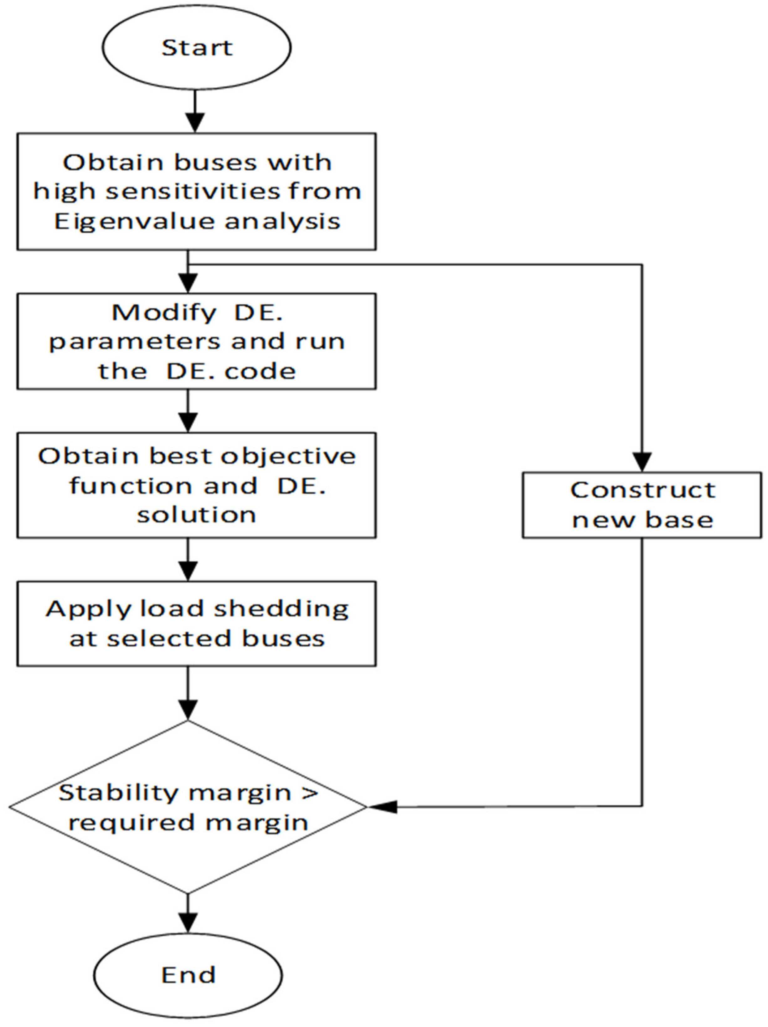
2. Methodology
2.1. Nodal Analysis and Participation Factor
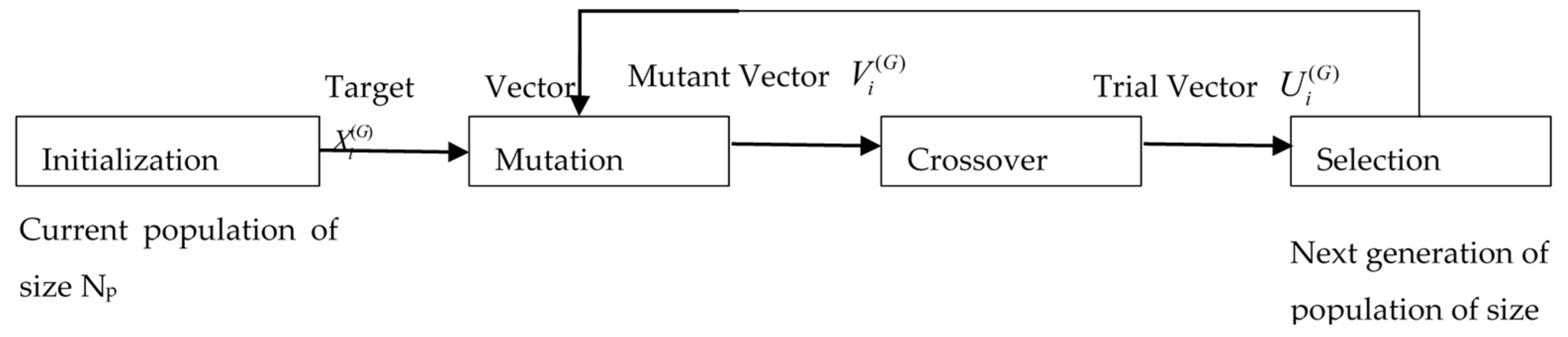
2.2. Differential Evolution
- Initialization
- Mutation
- Crossover
- Selection
2.3. Genetic Algorithm Solution Space
- Encoding. Encoding is the representation of chromosomes (different voltages at the nodes), which establishes the mapping between the solution space of the original problem and the environment of the population in GA. The form of encoding is related to the characteristics of the original problem’s decision variables.
- Population initialization. Population initialization is used to obtain initial solutions and prepare for the subsequent evolution.
- Fitness function. Fitness function is designed according to the original problem’s objective function, and the fitness function value of a chromosome determines the probability of its retention.
- Genetic operators. Genetic operators include the selection operator, crossover operator, and mutation operator. The selection operator selects chromosomes from the current population to enter the next generation population.
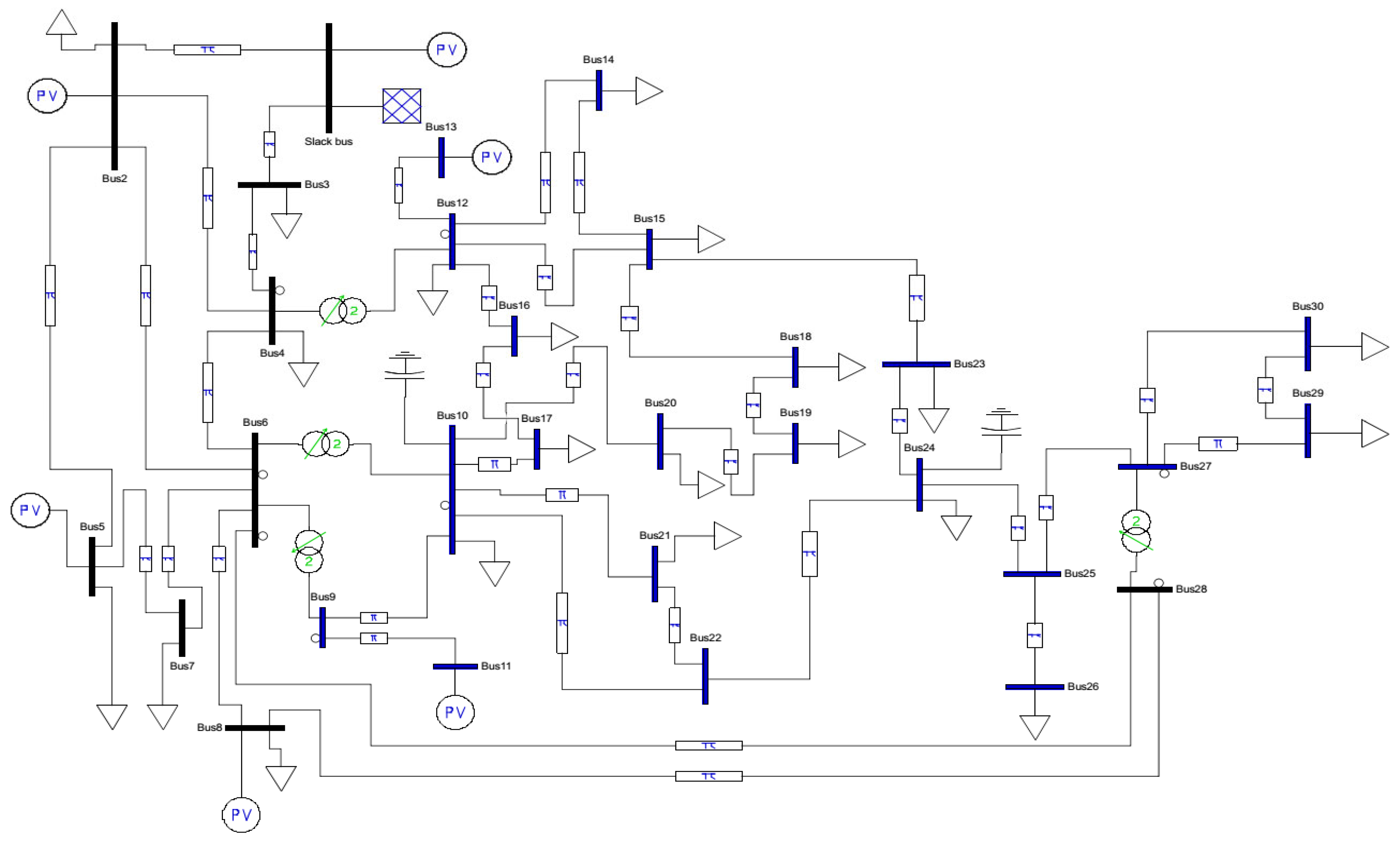
3. Numerical Simulation
4. Results and Discussion
5. Conclusions
- A simulation was performed on the grid, using PSAT for nodal load analysis to identify the critical load buses.
- A computational algorithm was developed for load shedding, based on the sensitivities of the load bus using differential evolution, and was validated using a genetic algorithm.
- The results proved that DE significantly improved the voltage profile of the test bus system after load shedding, with a percentage improvement of 10.6, 8.7, and 13.4 on buses 26, 29, and 30, respectively, as opposed to 10.2, 7.6, and 13.1 on the same buses, using GA.
- The system network also experienced an appropriate increment in voltage values per unit at the selected load buses and other subsequent buses.
Author Contributions
Funding
Institutional Review Board Statement
Informed Consent Statement
Data Availability Statement
Acknowledgments
Conflicts of Interest
References
- Gbadamosi, S.L.; Nwulu, N.I. A multi-period composite generation and transmission expansion planning model incorporating renewable energy sources and demand response. Sustain. Energy Technol. Assess. 2020, 39, 100726. [Google Scholar] [CrossRef]
- Gbadamosi, S.L.; Nwulu, N.I. A comparative analysis of generation and transmission expansion planning models for power loss minimization. Sustain. Energy Grids Netw. 2021, 26, 100456. [Google Scholar] [CrossRef]
- Gbadamosi, S.L.; Nwulu, N.I. Reliability assessment of composite generation and transmission expansion planning incorporating renewable energy sources. J. Renew. Sustain. Energy 2020, 12, 026301. [Google Scholar] [CrossRef]
- Gbadamosi, S.L.; Nwulu, N.I.; Sun, Y. Multi-objective optimisation for composite generation and transmission expansion planning considering offshore wind power and feed-in tariffs. IET Renew. Power Gener. 2018, 12, 1687–1697. [Google Scholar] [CrossRef]
- Deng, J.; Liu, J. A Study on a Centralized Under-Voltage Load Shedding Scheme Considering the Load Characteristics. Phys. Procedia 2012, 24, 481–489. [Google Scholar] [CrossRef] [Green Version]
- Arief, A.; Dong, Z.; Nappu, M.B.; Gallagher, M. Under voltage load shedding in power systems with wind turbine-driven doubly fed induction generators. Electr. Power Syst. Res. 2013, 96, 91–100. [Google Scholar] [CrossRef] [Green Version]
- Larik, R.; Mustafa, M.W.; Aman, M.; Jumani, T.; Sajid, S.; Panjwani, M. An Improved Algorithm for Optimal Load Shedding in Power Systems. Energies 2018, 11, 1808. [Google Scholar] [CrossRef] [Green Version]
- Wiszniewski, A. New criteria of voltage stability margin for the purpose of load shedding. IEEE Trans. Power Deliv. 2007, 22, 1367–1371. [Google Scholar] [CrossRef] [Green Version]
- Jallad, J.; Mekhilef, S.; Mokhlis, H.; Laghari, J.; Badran, O. Application of Hybrid Meta-Heuristic Techniques for Optimal Load Shedding Planning and Operation in an Islanded Distribution Network Integrated with Distributed Generation. Energies 2018, 11, 1134. [Google Scholar] [CrossRef] [Green Version]
- Mageshvaran, R.; Jayabarathi, T. GSO based optimization of steady state load shedding in power systems to mitigate blackout during generation contingencies. Ain Shams Eng. J. 2015, 6, 145–160. [Google Scholar] [CrossRef] [Green Version]
- Raghu, C.; Aravind, P.M. Assessing Effectiveness of Research for Load Shedding in Power System. Int. J. Electr. Comput. Eng. 2017, 7, 3235–3245. [Google Scholar]
- Cui, L.; Wang, L.; Deng, J.; Zhang, J. Intelligent algorithms for a new joint replenishment and synthetical delivery problem in a warehouse centralized supply chain. Knowl.-Based Syst. 2015, 90, 185–198. [Google Scholar] [CrossRef]
- Wang, L.; Dun, C.X.; Bi, W.J.; Zeng, Y.R. An effective and efficient differential evolution algorithm for the integrated stochastic joint replenishment and delivery model. Knowl.-Based Syst. 2012, 36, 104–114. [Google Scholar] [CrossRef]
- Qu, H.; Ai, X.Y.; Wang, L. Optimizing an integrated inventory-routing system for multi-item joint replenishment and coordinated outbound delivery using differential evolution algorithm. Appl. Soft Comput. 2020, 86, 105863. [Google Scholar] [CrossRef]
- Ajmal, M.S.; Iqbal, Z.; Khan, F.Z.; Ahmad, M.; Ahmad, I.; Gupta, B.B. Hybrid ant genetic algorithm for efficient task scheduling in cloud data centers. Comput. Electr. Eng. 2021, 95, 107419. [Google Scholar] [CrossRef]
- Liu, Y.; Ćetenović, D.; Li, H.; Gryazina, E.; Terzia, V. An optimized multi-objective reactive power dispatch strategy based on improved genetic algorithm for wind power integrated systems. Int. J. Electr. Power Energy Syst. 2022, 136, 107764. [Google Scholar] [CrossRef]
- Yuan, H.-B.; Zou, W.-J.; Jung, S.; Kim, Y.-B. Optimized rule-based energy management for a polymer electrolyte membrane fuel cell/battery hybrid power system using a genetic algorithm. Int. J. Hydrogen Energy 2022, 47, 7932–7948. [Google Scholar] [CrossRef]
- Ramos-Figueroa, O.; Quiroz-Castellanos, M.; Mezura-Montes, E.; Kharel, R. Variation Operators for Grouping Genetic Algorithms: A Review. Swarm Evolut. Comput. 2021, 60, 100796. [Google Scholar] [CrossRef]
- Kothari, D.P.; Nagrath, I.J. Modern Power System Analysis; McGraw Hill Education: New York, NY, USA, 2003. [Google Scholar]
- Jegatheesan, R.; Nor, N.M.; Romlie, M.F. Newton-Raphson power flow solution employing systematically constructed jacobian matrix. In Proceedings of the 2nd IEEE International Conference on Power and Energy (PECON 08), Johor Bahru, Malaysia, 1–3 December 2008. [Google Scholar]
- Konoval, V.; Prytula, R. Participation Factor in Modal Analysis of Power System Stability. Pozn. Univ. Technol. Acad. J. 2016, 86, 97–104. [Google Scholar]
- Enemuoh, F.O.; Onuegbu, J.C.; Anazie, E.A. Modal based analysis of and Evaluation of Voltage Stability of Bulk Power System. Int. J. Eng. Res. Dev. 2013, 6, 71–79. [Google Scholar]
- Tao, Z.; Moncada, J.A.; Poncelet, K.; Delarue, E. Review and analysis of investment decision making algorithms in long-term agent-based electric power system simulation models. Renew. Sustain. Energy Rev. 2021, 136, 110405. [Google Scholar] [CrossRef]
- Xu, L. Research on computer interactive optimization design of power system based on genetic algorithm. Energy Rep. 2021, 7, 1–13. [Google Scholar] [CrossRef]
- Milano, F. Documentation for PSAT, Version 2.0.0; University of Castilla-La Mancha: Ciudad Real, Spain, 2008. [Google Scholar]

| Bus | V (p.u) | Phase (p.u) | PG (p.u) | QG (p.u) | PL (p.u) | QL (p.u) |
|---|---|---|---|---|---|---|
| 1 | 1 | 0 | 0.5695 | −0.171 | 0 | 0 |
| 2 | 1 | −0.0123 | 0.8 | −0.0031 | 0.217 | 0.127 |
| 3 | 0.994 | −0.0467 | 0 | 0 | 0.024 | 0.012 |
| 4 | 0.9918 | −0.0555 | 0 | 0 | 0.076 | 0.016 |
| 5 | 1 | −0.0875 | 0.5 | 0.3738 | 0.942 | 0.19 |
| 6 | 0.9885 | −0.0713 | 0 | 0 | 0 | 0 |
| 7 | 0.9838 | −0.0848 | 0 | 0 | 0.228 | 0.109 |
| 8 | 1 | −0.0741 | 0.35 | 0.418 | 0.3 | 0.3 |
| 9 | 0.9781 | −0.0899 | 0 | 0 | 0 | 0 |
| 10 | 0.9575 | −0.138 | 0 | 0 | 0.058 | −0.1542 |
| 11 | 1 | −0.0529 | 0.3 | 0.0846 | 0 | 0 |
| 12 | 0.9849 | −0.0654 | 0 | 0 | 0.112 | 0.075 |
| 13 | 1 | −0.0535 | 0.4 | 0.258 | 0 | 0 |
| 14 | 0.9321 | −0.1189 | 0 | 0 | 0.062 | 0.016 |
| 15 | 0.904 | −0.1213 | 0 | 0 | 0.082 | 0.025 |
| 16 | 0.9513 | −0.1045 | 0 | 0 | 0.035 | 0.018 |
| 17 | 0.9344 | −0.1484 | 0 | 0 | 0.09 | 0.058 |
| 18 | 0.7854 | −0.1631 | 0 | 0 | 0.0308 | 0.0867 |
| 19 | 0.8211 | −0.2052 | 0 | 0 | 0.095 | 0.034 |
| 20 | 0.8519 | −0.1918 | 0 | 0 | 0.022 | 0.007 |
| 21 | 0.925 | −0.1652 | 0 | 0 | 0.175 | 0.112 |
| 22 | 0.9249 | −0.1647 | 0 | 0 | 0 | 0 |
| 23 | 0.8459 | −0.1855 | 0 | 0 | 0.032 | 0.016 |
| 24 | 0.835 | −0.2208 | 0 | 0 | 0.087 | 0.0391 |
| 25 | 0.886 | −0.1957 | 0 | 0 | 0 | 0 |
| 26 | 0.7543 | −0.2577 | 0 | 0 | 0.0311 | 0.0204 |
| 27 | 0.984 | −0.1495 | 0 | 0 | 0 | 0 |
| 28 | 0.9862 | −0.0802 | 0 | 0 | 0 | 0 |
| 29 | 0.818 | −0.2999 | 0 | 0 | 0.024 | 0.009 |
| 30 | 0.7301 | −0.4294 | 0 | 0 | 0.0883 | 0.0158 |
| Eigenvalue | Most Associated | Real Part | Imaginary Part |
|---|---|---|---|
| 1 | 4 | 101.2515 | 0 |
| 2 | 6 | 68.8145 | 0 |
| 3 | 12 | 35.2022 | 0 |
| 4 | 21 | 30.7752 | 0 |
| 5 | 10 | 26.7856 | 0 |
| 6 | 28 | 23.2185 | 0 |
| 7 | 7 | 18.2507 | 0 |
| 8 | 9 | 13.8303 | 0 |
| 9 | 20 | 9.0177 | 0 |
| 10 | 3 | 8.3785 | 0 |
| 11 | 15 | 4.5032 | 0 |
| 12 | 17 | 4.3497 | 0 |
| 13 | 27 | 3.6812 | 0 |
| 14 | 16 | 2.4336 | 0 |
| 15 | 16 | 1.9424 | 0 |
| 16 | 24 | 1.9531 | 0 |
| 17 | 14 | 1.5499 | 0 |
| 18 | 25 | 1.3671 | 0 |
| 19 | 30 | 0.1105 | 0 |
| 20 | 26 | 0.1691 | 0 |
| 21 | 18 | 0.3376 | 0 |
| 22 | 23 | 1.1136 | 0 |
| 23 | 23 | 0.6299 | 0 |
| 24 | 29 | 0.7744 | 0 |
| 25 | 11 | 999 | 0 |
| 26 | 13 | 999 | 0 |
| 27 | 2 | 999 | 0 |
| 28 | 5 | 999 | 0 |
| 29 | 8 | 999 | 0 |
| 30 | Slack Bus | 1998 | 0 |
| Bus | Participation Factor |
|---|---|
| Slack bus | 0 |
| 2 | 0 |
| 3 | 0 |
| 4 | 0 |
| 5 | 0 |
| 6 | 0.0001 |
| 7 | 0.0001 |
| 8 | 0 |
| 9 | 0.0001 |
| 10 | 0.0003 |
| 11 | 0 |
| 12 | 0 |
| 13 | 0 |
| 14 | 0.0001 |
| 15 | 0.0003 |
| 16 | 0.0001 |
| 17 | 0.0003 |
| 18 | 0.0009 |
| 19 | 0.0008 |
| 20 | 0.0007 |
| 21 | 0.0007 |
| 22 | 0.0008 |
| 23 | 0.0038 |
| 24 | 0.0103 |
| 25 | 0.0514 |
| 26 | 0.2287 |
| 27 | 0.0205 |
| 28 | 0.0006 |
| 29 | 0.2545 |
| 30 | 0.4251 |
| Bus | Initial Active Power | Minimum Load Shed | Maximum Load Shed | Total Load Shed | Active Power after Optimized Load Shedding (p.u.) | Reactive Power after Optimized Load Shedding (p.u.) |
|---|---|---|---|---|---|---|
| 26 | 0.035 | 0.007 | 0.0245 | 0.0035 | 0.0315 | 0.0207 |
| 29 | 0.024 | 0.0048 | 0.0168 | 0.0024 | 0.0216 | 0.0081 |
| 30 | 0.106 | 0.0212 | 0.0742 | 0.0106 | 0.0954 | 0.0171 |
| Bus | Phase (p.u.) | PG (p.u.) | QG (p.u.) | PL (p.u.) | QL (p.u.) |
|---|---|---|---|---|---|
| Slack Bus | 0 | 0.453 | −0.1539 | 0 | 0 |
| 2 | −0.009 | 0.8 | −0.0314 | 0.217 | 0.127 |
| 3 | −0.0396 | 0 | 0 | 0.024 | 0.012 |
| 4 | −0.047 | 0 | 0 | 0.076 | 0.016 |
| 5 | −0.081 | 0.5 | 0.3606 | 0.942 | 0.19 |
| 6 | −0.061 | 0 | 0 | 0 | 0 |
| 7 | −0.0755 | 0 | 0 | 0.228 | 0.109 |
| 8 | −0.0619 | 0.35 | 0.3674 | 0.3 | 0.3 |
| 9 | −0.0722 | 0 | 0 | 0 | 0 |
| 10 | −0.1175 | 0 | 0 | 0.058 | −0.1579 |
| 11 | −0.0341 | 0.3 | 0.0518 | 0 | 0 |
| 12 | −0.049 | 0 | 0 | 0.112 | 0.075 |
| 13 | −0.0366 | 0.4 | 0.2196 | 0 | 0 |
| 14 | −0.0989 | 0 | 0 | 0.0606 | 0.0156 |
| 15 | −0.1004 | 0 | 0 | 0.077 | 0.0235 |
| 16 | −0.0868 | 0 | 0 | 0.035 | 0.018 |
| 17 | −0.128 | 0 | 0 | 0.0889 | 0.0573 |
| 18 | −0.1356 | 0 | 0 | 0.0246 | 0.0692 |
| 19 | −0.1686 | 0 | 0 | 0.078 | 0.0279 |
| 20 | −0.159 | 0 | 0 | 0.0191 | 0.0061 |
| 21 | −0.1424 | 0 | 0 | 0.1708 | 0.1093 |
| 22 | −0.1415 | 0 | 0 | 0 | 0 |
| 23 | −0.1548 | 0 | 0 | 0.0273 | 0.0137 |
| 24 | −0.1859 | 0 | 0 | 0.074 | 0.0263 |
| 25 | −0.1596 | 0 | 0 | 0 | 0 |
| 26 | −0.2014 | 0 | 0 | 0.0243 | 0.016 |
| 27 | −0.1213 | 0 | 0 | 0 | 0 |
| 28 | −0.0681 | 0 | 0 | 0 | 0 |
| 29 | −0.231 | 0 | 0 | 0.0189 | 0.0071 |
| 30 | −0.3177 | 0 | 0 | 0.0725 | 0.013 |
| Bus | V (before Load Shedding) (p.u.) | V (after Load Shedding) (p.u.) | Percentage Improvement Using GA | Percentage Improvement Using DE |
|---|---|---|---|---|
| Slack Bus | 1.0000 | 1.0000 | 0 | 0 |
| 2 | 1.0000 | 1.0000 | 0 | 0 |
| 3 | 0.9940 | 0.9961 | 0.2005 | 0.2062 |
| 4 | 0.9918 | 0.9943 | 0.2101 | 0.2563 |
| 5 | 1.0000 | 1.0000 | 0 | 0 |
| 6 | 0.9885 | 0.9918 | 0.2689 | 0.3312 |
| 7 | 0.9838 | 0.9863 | 0.2180 | 0.2484 |
| 8 | 1.0000 | 1.0000 | 0 | 0 |
| 9 | 0.9781 | 0.9825 | 0.3897 | 0.4441 |
| 10 | 0.9575 | 0.9676 | 1.0435 | 1.0501 |
| 11 | 1.0000 | 1.0000 | 0 | 0 |
| 12 | 0.9849 | 0.9863 | 0.0564 | 0.1484 |
| 13 | 1.0000 | 1.0000 | 0 | 0 |
| 14 | 0.9321 | 0.9390 | 0.7041 | 0.7441 |
| 15 | 0.9040 | 0.9205 | 1.0118 | 1.8322 |
| 16 | 0.9513 | 0.9557 | 0.4443 | 0.4646 |
| 17 | 0.9344 | 0.9440 | 1.0000 | 1.0246 |
| 18 | 0.7854 | 0.8330 | 4.6387 | 6.0636 |
| 19 | 0.8211 | 0.8608 | 2.8586 | 4.8275 |
| 20 | 0.8519 | 0.8848 | 1.5174 | 3.8585 |
| 21 | 0.9250 | 0.9385 | 1.4156 | 1.4542 |
| 22 | 0.9249 | 0.9392 | 1.3692 | 1.5564 |
| 23 | 0.8459 | 0.8782 | 1.4397 | 3.8156 |
| 24 | 0.8350 | 0.8762 | 3.1472 | 4.9397 |
| 25 | 0.8860 | 0.9267 | 2.1168 | 4.5927 |
| 26 | 0.7543 | 0.8342 | 10.2000 | 10.5823 |
| 27 | 0.9840 | 1.0043 | 2.0124 | 2.0583 |
| 28 | 0.9862 | 0.9914 | 0.4596 | 0.5240 |
| 29 | 0.8180 | 0.8893 | 7.5706 | 8.7188 |
| 30 | 0.7301 | 0.8280 | 13.1040 | 13.4060 |
Publisher’s Note: MDPI stays neutral with regard to jurisdictional claims in published maps and institutional affiliations. |
© 2022 by the authors. Licensee MDPI, Basel, Switzerland. This article is an open access article distributed under the terms and conditions of the Creative Commons Attribution (CC BY) license (https://creativecommons.org/licenses/by/4.0/).
Share and Cite
Amusan, O.T.; Nwulu, N.I.; Gbadamosi, S.L. Identification of Weak Buses for Optimal Load Shedding Using Differential Evolution. Sustainability 2022, 14, 3146. https://doi.org/10.3390/su14063146
Amusan OT, Nwulu NI, Gbadamosi SL. Identification of Weak Buses for Optimal Load Shedding Using Differential Evolution. Sustainability. 2022; 14(6):3146. https://doi.org/10.3390/su14063146
Chicago/Turabian StyleAmusan, Olumuyiwa T., Nnamdi I. Nwulu, and Saheed Lekan Gbadamosi. 2022. "Identification of Weak Buses for Optimal Load Shedding Using Differential Evolution" Sustainability 14, no. 6: 3146. https://doi.org/10.3390/su14063146
APA StyleAmusan, O. T., Nwulu, N. I., & Gbadamosi, S. L. (2022). Identification of Weak Buses for Optimal Load Shedding Using Differential Evolution. Sustainability, 14(6), 3146. https://doi.org/10.3390/su14063146