Depth-Wise Separable Convolution Attention Module for Garbage Image Classification

Abstract

Currently, how to deal with the massive garbage produced by various human activities is a hot topic all around the world. In this paper, a preliminary and essential step is to classify the garbage into different categories. However, the mainstream waste classification mode relies heavily on manual work, which consumes a lot of labor and is very inefficient. With the rapid development of deep learning, convolutional neural networks (CNN) have been successfully applied to various application fields. Therefore, some researchers have directly adopted CNNs to classify garbage through their images. However, compared with other images, the garbage images have their own characteristics (such as inter-class similarity, intra-class variance and complex background). Thus, neglecting these characteristics would impair the classification accuracy of CNN. To overcome the limitations of existing garbage image classification methods, a Depth-wise Separable Convolution Attention Module (DSCAM) is proposed in this paper. In DSCAM, the inherent relationships of channels and spatial positions in garbage image features are captured by two attention modules with depth-wise separable convolutions, so that our method could only focus on important information and ignore the interference. Moreover, we also adopt a residual network as the backbone of DSCAM to enhance its discriminative ability. We conduct the experiments on five garbage datasets. The experimental results demonstrate that the proposed method could effectively classify the garbage images and that it outperforms some classical methods.

1. Introduction

Due to the population increase and economic development, the amount of garbage produced every day is growing rapidly, especially in developing countries [1]. If such a large amount of garbage is not treated effectively, it will cause severe environmental pollution and a massive waste of resources. Efficient sorting, recycling, and regeneration treatment are the key and effective means to solve this problem. In recent years, more and more nations have started to explore recycling strategies to improve the environment with the ultimate goal of having a cyclical economy and sustainable development [2]. Scholars have done much research on the garbage classification problem. However, most of their proposed solutions focused on the terminal recycling method [3,4,5,6,7,8], which is highly dependent on people’s cooperation. At present, the most widely used garbage sorting method is based on manual classification. Although manual garbage classification could obtain highly accurate results, it is always time-consuming and requires well-trained operators, which seriously limits the efficiency of garbage classification. Therefore, the automated garbage sorting method is an effective way to solve this problem.

With the development of artificial intelligence (AI) technology, AI-related applications, such as computer vision, speech recognition and natural language processing, have been gaining more and more attention in many industries. Some researchers have also leveraged the artificial intelligence methods for garbage classification and sorting. Wang et al. [9] utilized support vector machine (SVM) [10] and boosting algorithm to classify garbage images. Similarly, Liu et al. [11] also combined multi-class SVM classifier with a speeded up robust feature (SURF) [12] to establish a smart waste sorting system. Though SVM can effectively accomplish the garbage classification task, it belongs to the shallow classification model. Thus, the classification result obtained by SVM may not be optimal. Recently, with the rapid development of deep learning, some deep convolutional neural network- (CNN) based methods were gradually incorporated into the garbage classification task to improve its accuracy. Ozkaya et al. [13] attempted to train different CNNs on a small garbage dataset with transfer learning, and then adopted an SVM to classify the feature obtained by CNNs. Similarly, Fu et al. [14] employed a transfer learning strategy to train a CNN model so that the classification accuracy of garbage images can be improved. Meng et al. [15] designed a network that can reuse and fuse features obtained by different layers of CNN, the multi-scale feature interaction in their method can significantly improve the classification performance. Singh [16] used a modified CNN model called Xception to accomplish the classification task for plastic bags. Besides, CNN has also been combined with some hardware to form various garbage classification systems. Nowakowski and Pamuła [17] proposed a region-based CNN algorithm to classify the garbage images so that the users can recognize the category of garbage by smartphones. Chu et al. [18] deployed a detection system for municipal solid waste recycling, which consists of a high-resolution camera, a bridge sensor, an inductor and a PC. This system takes the pictures of garbage and then utilizes a CNN for classification. In [19], Yu et al. proposed a deep CNN which fuses multiple features in multiple scales for solid garbage detection and sorting. Although Yu’s method can improve the detection accuracy by adding multi-view feature, it relies on expensive 3D camera hardware to get the depth information of garbage images. Kokoulin and Tur [20] integrated CNN with IoT hardware and a reverse vending machine (a device that accepts used beverage containers and returns money to the user) to classify and recycle beverage containers. Wang et al. [21] proposed a framework which first classifies the garbage images by a CNN and then monitors the operating state of garbage containers using smart sensors.

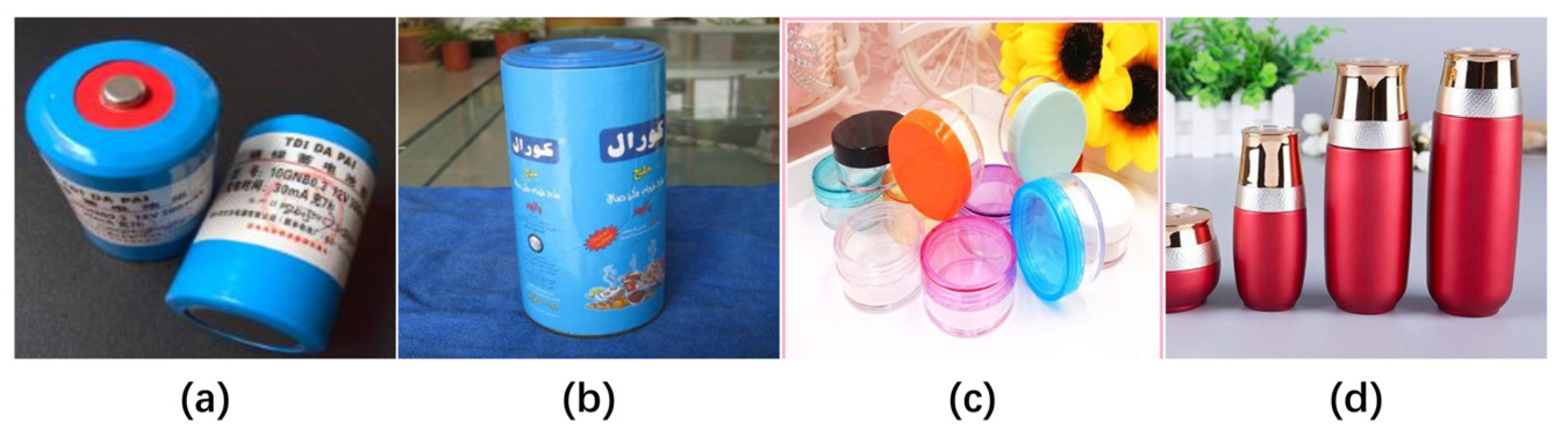
From the aforementioned works, it can be seen that classifying the garbage into their corresponding categories is a preliminary and important step in many garbage sorting and recycling tasks. However, the CNN models in most of the existing work (such as Alexnet, VGG and Xception used in [16,22,23]) were originally proposed for classifying natural images rather than garbage images. Hence, the characteristics of garbage images were neglected in them, which limits their performance. Actually, the garbage image classification is much more complicated than some other image classification tasks. For example, the accuracy of garbage image classification often suffers from the inter-class similarity and intra-class variance problem. 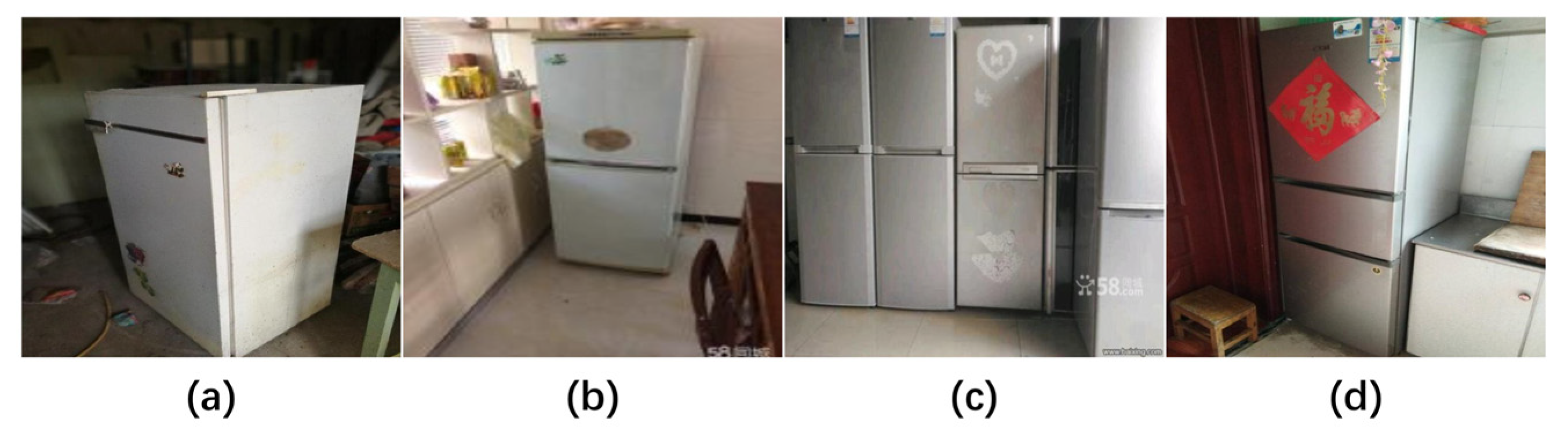That is, the appearance of some garbage belonging to different classes is more similar than those from the same class, as shown in Figure 1. Moreover, the various backgrounds around the target garbage will also impair the classification accuracy, as shown in Figure 2. To solve this problem, we introduce a new deep network named Depth-wise Separable Convolution Attention Module (DSCAM) in this paper. Compared with other studies [11,12,13,14,15], the proposed DSCAM is specially designed for garbage image classification in the following aspects. Firstly, in order to suppress the interference of other factors (such as the background) and make our model focus on the target garbage in images, an attention-based module is introduced into the proposed DSCAM. Secondly, unlike the existing work [13,14,15,16] which adopts the CNN models with only a small number of convolution layers to extract the feature of garbage image, we employ Resnet [24] as the backbone of our DSCAM. Since Resnet contains more convolution layers, the feature extraction ability of the proposed DSCAM can be enhanced to capture the discriminative features of garbage from different classes. At last, because the attention module and Resnet will bring more parameters into our model, the depth-wise separable convolution technique is used to compensate for the increase of computational burden. The effectiveness of the proposed method is demonstrated by extensive experiments on five garbage image classification datasets.

The rest of this paper is organized as follows: Section 2 briefly reviews some work related to our method. Section 3 presents the proposed DSCAM method. The experimental results on five datasets are shown and analyzed in Section 4. Finally, Section 5 concludes the paper.

2. Related Work

Deep convolutional neural networks (CNNs) have been widely used in the computer vision community and achieved remarkable progress in various tasks, e.g., image classification, object detection and semantic segmentation. Starting from the groundbreaking AlexNet [25] which successfully won the championship of ImageNet image classification in 2012, researchers have realized the importance of CNN for image feature extraction and have committed to further improving its performance [26,27]. The VGG [26] model has proved the importance of network depth in enhancing the effectiveness of CNN model. GoogLeNet [27] designed an Inception module so that the network could capture image features of different scales. Resnet [24] proposed a residual block with skipped connections to construct a deeper network architecture with more layers. Moreover, some other models have also been proposed to improve the performance of CNN in various aspects. For example, DenseNet [28] constructs connections in the CNN network so that the output feature of a layer can be regarded as the input of all its subsequent layers, which can improve the flow of information throughout the network to enhance the feature learning ability.

The attention mechanism has proved to be an effective way to promote the performance of deep CNNs. Thus, the incorporation of attention module into CNN has attracted a lot of interest [29,30]. One of the representative attention-based CNN methods is squeeze-and-excitation networks (SE-Net) [29], which learns channel attention for each convolutional block and brings apparent performance gain for various problems. Subsequently, some other attention modules were developed to enhance the feature aggregation or combine the channel and spatial attention. Specifically, CBAM [30] employed both average and max pooling to aggregate feature and fused channel and spatial attentions into one module, which achieves considerable performance improvements on many computer vision tasks.

To reduce the number of parameters and the computational burden of CNN, some efficient network models were proposed. Among these models, the most widely used are group convolutions [31,32,33] and depth-wise separable convolutions [34,35]. A group convolution can be viewed as a regular convolution with separable channel convolution kernels, where each kernel corresponds to a partition of channels without connections to other partitions. Xie et al. [32] and Zhang [33] used group convolutions to improve the architecture of the CNN network, which achieves better results while ensuring the number of parameters. Depth-wise separable convolution is an extension of the group convolution. Firstly, depth-wise separable convolution performs group convolution independently over each channel of the input feature, then a point-wise convolution, i.e., an $1\times 1$ convolution, is utilized to project the output of group convolution to a new channel space. The original idea of separable convolution operation comes from the Inception [27] network. Inspired by Inception, Chollet [34] proposed the Xception network, which uses depth-wise separable convolutional to further optimize the module structure and achieves satisfactory performance. The biggest benefit of depth-wise separable convolution is that it allows for significantly increasing the number of convolution units in a deep network without an uncontrolled blow-up in computational complexity. Thus, it has also been adopted in MobileNet [35] and ShuffleNet [36], which are designed for mobile device or embedded vision applications.

3. Proposed Network

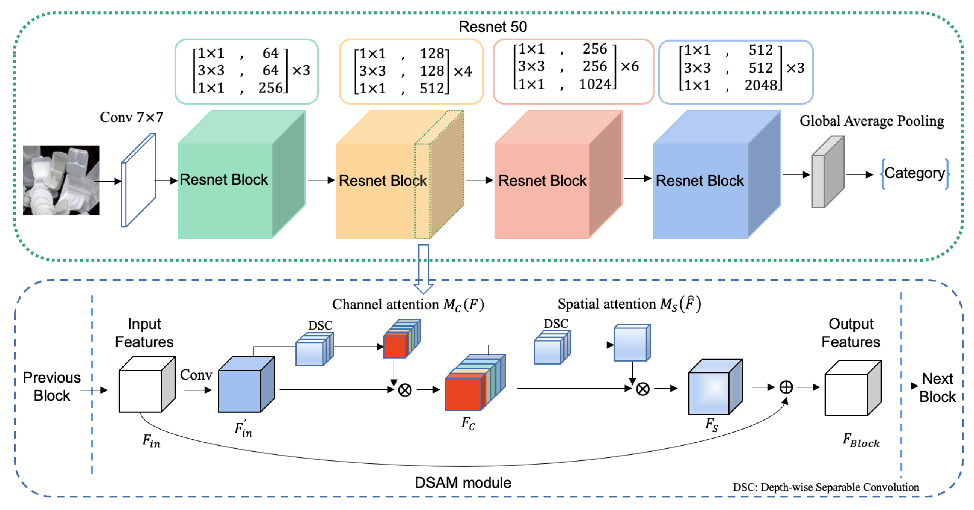
The whole structure of the proposed DSCAM is shown Figure 3. As can be seen from this figure, our DSCAM employs the Resnet-50 (i.e., Resnet with 50 layers) as its backbone. Compared with other CNN models with a small number of layers, Resnet introduces the “shortcut connections” that skip several network layers to avoid the vanishing gradient during network training. Thus, it can construct a deeper network with more layers to better extract discriminative features from the garbage images. In our network, the initial feature of input garbage image is first obtained by a shallow convolutional layer with kernel size of 7 × 7. Then, the shallow feature is inputted into four Resnet blocks for feature refining. In our work, an attention module is embedded in each sub-block of Resnet. The attention module has two sequential processes: channel attention and spatial attention. Each process adopts the depth-wise separable convolution to obtain an attention map which consists of weights to indicate the importance of each channel and spatial position. Through point-wise multiplying the feature with attention maps, our network could adaptively emphasize the informative objects in the garbage image and suppress irrelevant background. At last, a global average pooling layer and cross-entropy loss are employed for image classification. The details of a depth-wise separable convolution and attention module will be described in Section 3.1 and Section 3.2.

3.1. Depth-Wise Separable Convolution

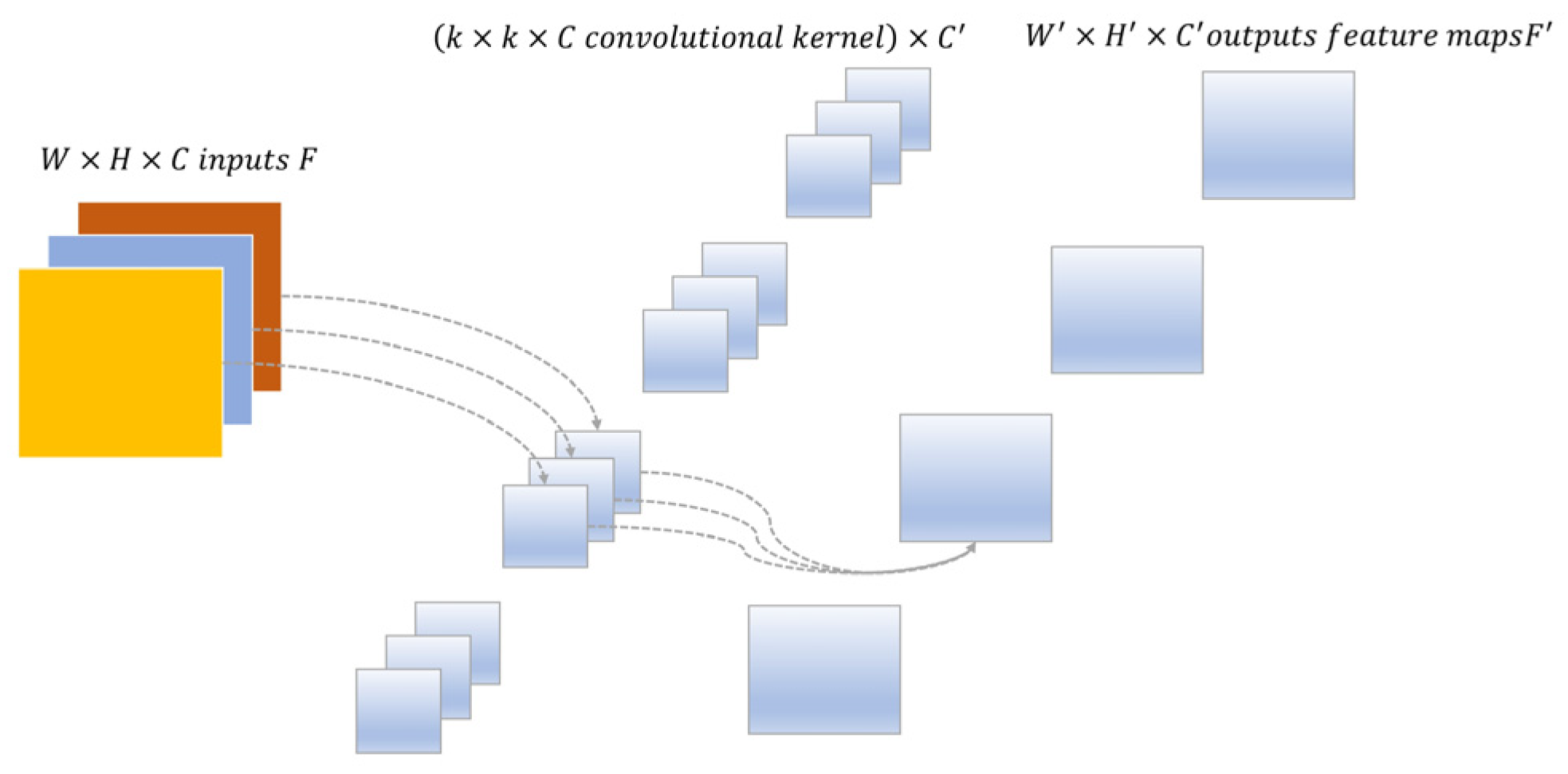
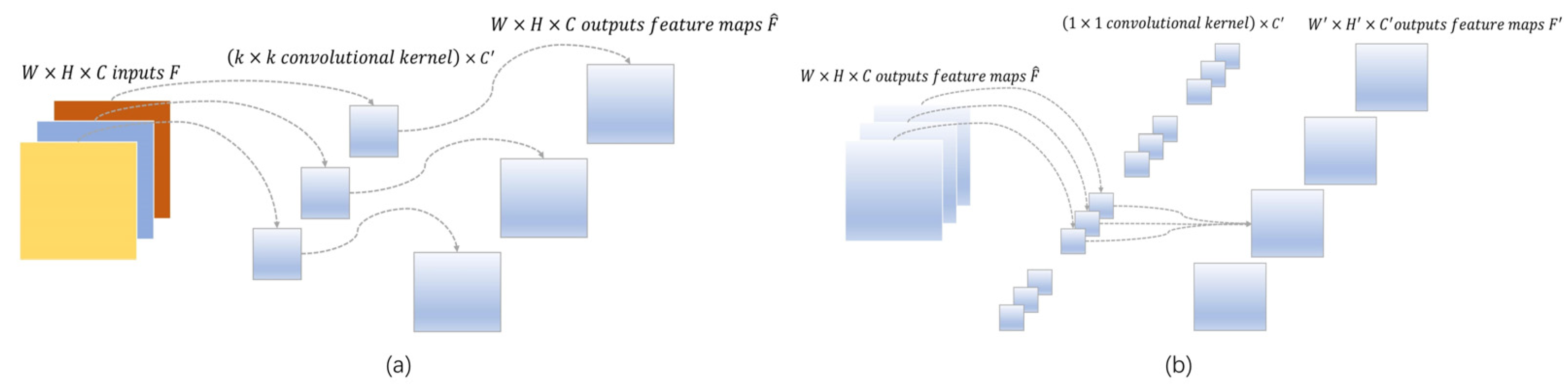
Here we briefly introduce how depth-wise separable convolution factorizes a standard convolution (as shown in Figure 4) into a depth convolution and a point-wise convolution ($1\times 1$ convolution). Given the input feature $F\in R^{W\times H\times C}$, where $W$ and $H$ denote the spatial dimensions and $C$ is the number of channels, through a standard convolution with kernel size $k\times k\times C\times C^{\prime }$, we can get the output $F^{\prime }\in R^{W^{\prime }\times H^{\prime }\times C^{\prime }}$, where $W^{\prime }$ and $H^{\prime }$ denote the spatial dimensions of $F^{\prime }$ and $C^{\prime }$ is the number of output channels.

In order to reduce the computational burden and parameters in standard convolution, depth-wise separable convolution first uses a depth-wise convolution (one filter per input channel) to convolve with the input feature, as shown in Figure 5a, which can be formularized as:

$$\widehat{F}=F\otimes K$$

(1)

where $F\in R^{W\times H\times C}$ is the input, $K=R^{k\times k\times C}$ is the depth-wise convolution kernel, is the convolution operation. Note that the output $\widehat{F}$ has the same number of channels as the input feature. Then, an additional point-wise convolution with a $1\times 1$ convolution kernel is applied to the output of the depth-wise convolution as shown in Figure 5b, which can be formularized as:

$$F^{\prime }=\widehat{F}\otimes \overline{K}$$

(2)

where $\widehat{F}\in R^{W\times H\times C}$ is the outputs of depth convolution, $\overline{K}=R^{1\times 1\times C\times C^{\prime }}$ is an $1\times 1$ convolution and $F^{\prime }\in R^{W^{\prime }\times H^{\prime }\times C^{\prime }}$ is the output of whole depth-wise separable convolution.

For standard convolution with the kernel size of $k\times k\times C\times C^{\prime }$, the number of parameters which needs to be optimized is $P_{std}=k^2\times C\times C^{\prime }$. On the contrary, a depth-wise separable convolution can reduce the number of parameters to $P_{ds}=k\times k\times C+C\times C^{\prime }=\left(k^2+C^{\prime }\right)\times C$. Thus, the ratio between them is $\frac{P_{ds}}{P_{std}}=\frac{1}{C^{\prime }}+\frac{1}{k^2}$. In real-world applications, the number of output channels and kernel size are usually much larger than $1$ (i.e., $1<<C^{\prime }$, $1<<k^2$). Thus, the depth-wise separable convolution can effectively compress the number of parameters and computational burden in a convolutional network. Moreover, some studies have also shown that depth-wise separable convolution could improve the classification performance of a network due to the cross-channel and spatial features being sufficiently decoupled and separately handled in it [34,35].

3.2. Depth-Wise Separable Convolution Attention Module

In this section, we mainly describe how to extract channel and spatial attention weights using depth-wise separable convolution.

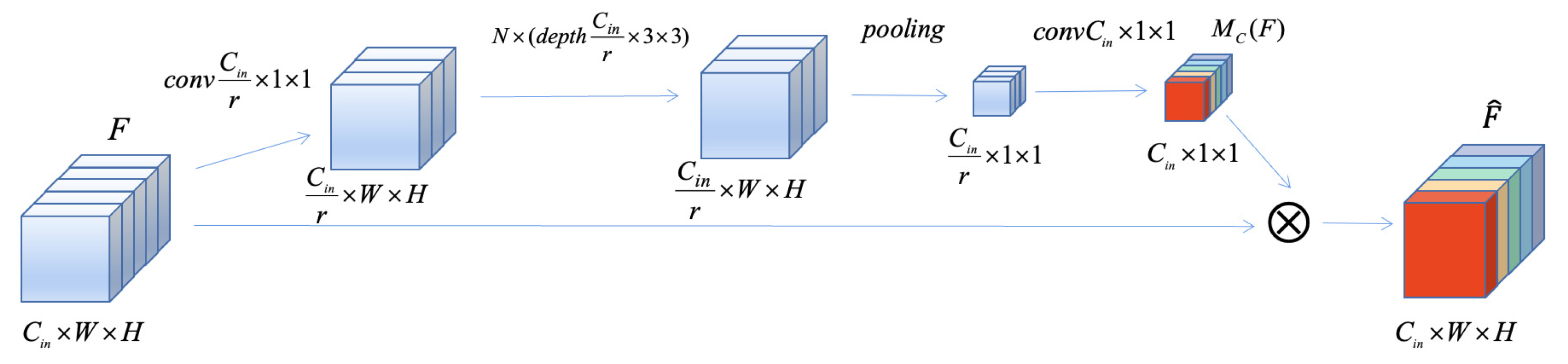
First, our purpose is to extract the channel attention weights which model interdependencies between channels. For arbitrary input features, a point-wise convolution is employed to fuse the information of different channels and reduce the dimension of channels to 1/r. After that, multiple depth convolution layers are used to extract local spatial information, and a max-pooling operation is utilized to squeeze the spatial dimension to $1$. Next, a $1\times 1$ convolution kernel is adopted to recover the channel dimension to the input feature dimension and obtain the specific channel attention weights $M_C(F)$. Finally, the input feature is multiplied by the channel attention weights in each channel to generate the weighted feature. The entire process is demonstrated in Figure 6.

The procedure of obtaining channel attention weights can be formularized as follows:

$$M_C\left(F\right)=\overline{W}\left(f_{{}_{pooling}}^s\left(W_g\left(W_p\left(F\right)\right)\right)\right)$$

(3)

where $F\in R^{W\times H\times C_{in}}$ is the input feature. $W_p$ is point-wise convolution operation which reduces the input dimension from $W\times H\times C_{in}$ to $\frac{W\times H\times C_{in}}{r}$, where (in Figure 6) represents the reduction ratio. $W_g$ is $N$ times depth convolution. $f_{pooling}^s$ is a spatial max-pooling operation and $\overline{W}$ denotes an $1\times 1$ convolution followed by a Sigmoid activation function, which ensures the channel dimension of the output feature is the same as the input. All convolution operations mentioned above are followed by the ReLU activation function (except the specific one mentioned).

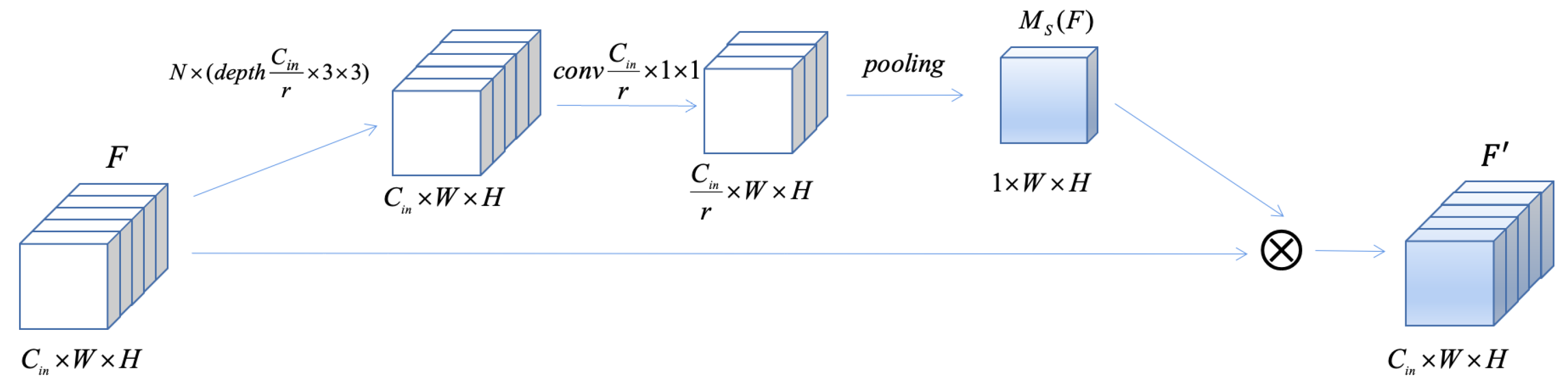
Second, we describe the process for spatial attention weights extraction. To calculate the internal relationship of features in space, multiple depth convolution operations are first performed on the input feature. Then, we utilize a point-wise convolution operation to reduce the channel dimension so that the channel information can be fused. After the pooling operation along the channel axis, we can obtain the spatial attention weights $M_S(F)$. Lastly, the input feature is multiplied by spatial attention weights in a point-wise manner to obtain the weighted feature. These operations are shown in Figure 7.

The procedure of spatial attention weights computation can be formularized as follows:

$$M_S\left(F\right)=f_{{}_{pooling}}^c\left(\left(W_p\left(W_g\left(F\right)\right)\right)\right)$$

(4)

where $W_g$ denotes $N$ times depth convolution operations, $W_P$ is a $1\times 1$ point-wise convolution, r is the reduction ratio, $f_{pooling}^c$ is the pooling operation along the channel axis. All convolution operations mentioned above are followed by the ReLU activation function, and we use max-pooling for all pooling operations.

3.3. DSCAM Block in Resnet

In this study, we integrate DSCAM into Resnet-50, thus each block in Resnet-50 can be formularized by Equations (5)–(8). In the notation that follows, we take $f_{conv}$ in Equation (5) to be a standard convolution operation, which convolves the input feature $F_{in}$ to $F_{in}^{\prime }$. Equations (6) and (7) are used to sequentially compute the weighted channel attention feature $F_C$ and weighted spatial attention feature $F_S$. In order to avoid the loss of information and make the network converge rapidly, we employ a skip connection to fuse the input $F_{in}$ with the feature $F_S$ by an element-wise summation (denoted by $\oplus$) in Equation (8), so that the final output $F_{Block}$ of the current Resnet block can be obtained.

$$F_{in}^{\prime }=f_{conv}\left(F_{in}\right)$$

(5)

$$F_C=M_C\left(F_{in}^{\prime }\right)\otimes F_{in}^{\prime }$$

(6)

$$F_S=M_S\left(F_C\right)\otimes F_C$$

(7)

$$F_{Block}=F_{in}\oplus F_S$$

(8)

3.4. Classification

To classify the feature of input garbage image, we use cross-entropy as the final loss function, which can be defined as:

$$Z=Softmax(f_{Avgpool}(F_{Block}^{\prime }))$$

(9)

$$L=-\frac{1}{T}{\displaystyle \sum _{i=1}^T{y}_i\ln Z_i}$$

(10)

In Equation (9), $F_{Block}^{\prime }$ denotes the output feature of the last convolution layer in Resnet-50 with attention modules, $f_{Avgpool}$ represents global average pooling operation, and the softmax function is defined as $Softmax\left(x\right)=exp(x_k)/{\displaystyle \sum _{k=1}^{M}exp(x_k)}$, where $M$ is the number of classes and $x_k$ is the k-th element of the output after average pooling. Through Equation (9), the classification result of the feature $F_{Block}^{\prime }$ can be obtained. For cross-entropy loss in Equation (10), $T$ denotes the total number of samples in training set, $Z_i$ represents the classification result of the i-th sample obtained by Equation (9) and $y_i$ is the true label (i.e., ground truth) of the i-th sample.

4. Experiments

In this section, we evaluate the effectiveness of our proposed method on garbage image datasets and compare its performance with other methods.

4.1. Garbage Datasets

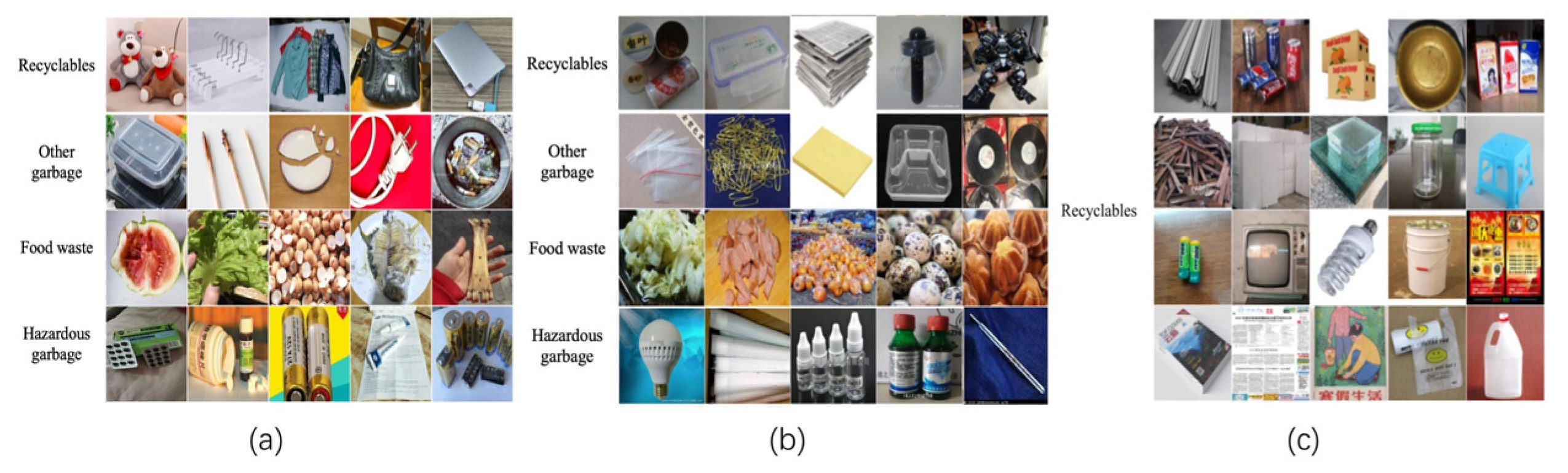
In this study, three publicly available garbage image datasets constructed by Huawei Cloud and Baidu AI Studio are employed to evaluate the performance of our proposed DSCAM.

The Huawei Garbage Classification Challenge Cup dataset (Huawei-40 for short) contains 18,112 images with 40 classes in total (eight types of food waste, 23 types of recyclables, six types of other garbage and three types of hazardous garbage, respectively), which are all common garbage in daily life. The image sizes vary from 113 × 76 to 4000 × 3000 in the Huawei-40 dataset, and the distribution of samples in each category is uneven, ranging from 50 images to 800 images per category.

Baidu’s garbage dataset (Baidu-214 for short) has 58,063 images belonging to 214 classes (106 types of recyclables, 53 types of food waste, 36 types of other garbage and 19 types of hazardous garbage, respectively). The minimum and maximum sizes of images in this dataset are $78\times 78$ and $6720\times 4480$. The number of images in each class ranges from 13 to 1654.

The Baidu recyclable garbage dataset (Baidu-RC for short) has 16,847 images from 21 recyclable garbage classes. The resolution of images in this dataset varies from $78\times 78$ to $8150\times 5315$, and the distribution of samples in Baidu-RC ranges from 250 images to 1000 images per category.

Some samples of the three datasets mentioned above are shown in Figure 8 (a), (b) and (c), respectively.

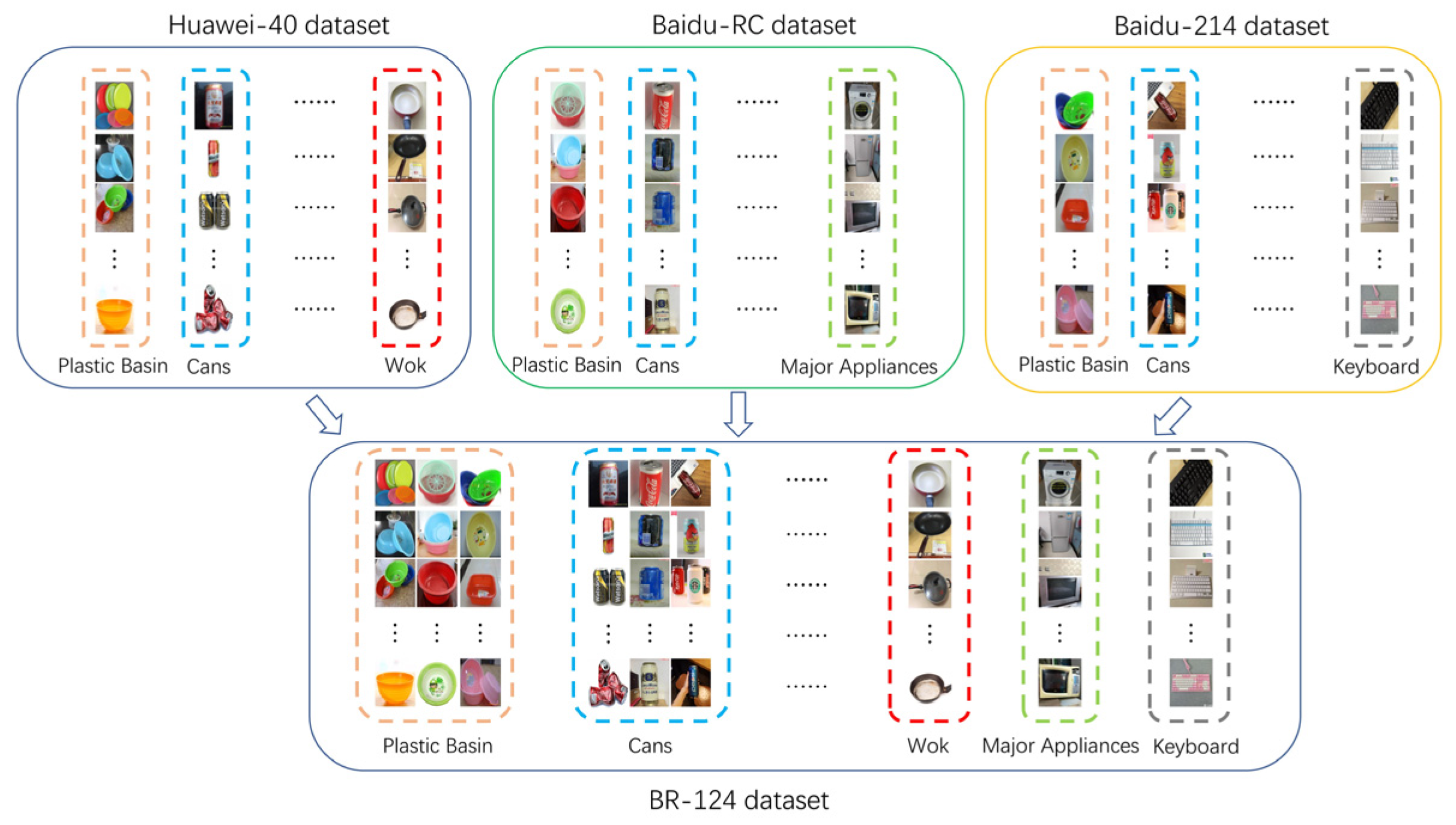
Because recyclable garbage is the most valuable among domestic garbage, we combine the recyclable garbage images from Huawei-40, Baidu-214, and Baidu-RC datasets to generate a new dataset named as BR-124 to further comprehensively evaluate our method’s performance. Specifically, we first select the images containing recyclable garbage from Huawei-40 and Baidu-214 datasets. Then, for the selected images whose categories exist in Baidu-RC dataset, we merge them with samples from the same category in Baidu-RC to form their corresponding categories in a new dataset. On the contrary, if the categories of some selected images are not included in Baidu-RC, they are directly put into the new BR-124 dataset. As a result, the BR-124 dataset contains 55,513 images distributed in 124 classes. The procedure of BR-124 dataset construction is shown in Figure 9.

Table 1. Dataset Attributes.

Dataset	Number of Samples	Number of Categories
Huawei-40 dataset	19,735	40
Baidu-214 dataset	58,063	214
Baidu-RC dataset	16,847	21
BR-124 dataset	55,513	124

summarizes the information of datasets used in this experiment.

For all the above datasets, we convert the class label of each image into a one-hot vector (a vector has the same length as the number of categories, in which the i-th element is set to 1 if the garbage image belongs to the i-th class and the rest are all set to 0). All images are resized to $224\times 224\times 3$, where 224 is the image size, 3 is the number of RGB color channels.

4.2. Experimental Setup

In the experiment, all networks were implemented using the Pytorch framework and performed on two NVIDIA GeForce RTX 2080 Ti GPUs. We randomly selected 90% samples from each garbage dataset as the training set and the remaining 10% as the test set. The random selecting process is repeated five times, and then the average classification accuracy is reported. In addition, we use stochastic gradient descent (SGD) as the optimization method during the network training. The learning rate was initially set to 0.01 with a weight decay 0.0005 and Momentum 0.9. Then, we set the learning rate drops to 10% and 5% of its initial value at the 75th and 150th training iterations. Each drop in the learning rate can make the network fine-tuned locally.

4.3. Experimental Results

First, we compared our proposed network with some other widely used CNN architectures in garbage classification, including VGG-19 [23], Xception [34], X-DenseNet [15], MobileNet-V3 [37] and GNet [14]. From the classification accuracy of different methods in

Table 2. Classification accuracy (%) ± Standard deviation (%) obtained by different methods.

Methods	Huawei-40	Baidu-214	Baidu-RC	BR-124
VGG-19	84.96 ± 0.63	72.98 ± 0.61	86. 38 ± 0.47	79.13 ± 0.47
Xception	88.45 ± 0.65	79.09 ± 0.55	90.12 ± 0.52	82.88 ± 0.56
X-DenseNet	89.31 ± 0.59	80.38 ± 0.57	91.74 ± 0.46	83.53 ± 0.41
MobileNet-V3	90.83 ± 0.47	82.01 ± 0.63	92.48 ± 0.41	84.70 ± 0.51
GNet	90.99 ± 0.33	82.57 ± 0.43	92.63 ± 0.35	84.89 ± 0.46
DSCAM	91.20 ± 0.43	83.01 ± 0.48	92.77 ± 0.45	85.35 ± 0.43

, the following points can be found. The VGG-19 network has the lowest accuracy in all compared methods since it has a simple architecture and shallow layers. Xception adopts depth-wise separable convolution to construct a complex network with more layers. Thus, it achieves higher accuracy than VGG-19. X-DenseNet is an extension of Xception, which uses a dense block to realize feature reuse and fusion. Due to this advantage, X-DenseNet outperforms Xception on all datasets. Nevertheless, the network architecture of Xception and X-DenseNet do not contain any attention module, which leads them to ignore the different importance of extracted feature. For MobileNet-V3 and GNet, since they embed the SE attention module [19] into some layers of their network, we can find that their performance is better than Xception and X-DenseNet. However, SE attention only takes the channel information into account. Hence, the classification results of MobileNet-V3 and GNet are still inferior to the proposed DSCAM, in which both the channel and spatial attention are considered.

Then, to justify the effectiveness of each component in our DSCAM, we compare the proposed method with three other networks, including Resnet (the original Resnet-50 without attention), SE network and CBAM network. In SE network, we embed SE module in the last convolution layer of each Resnet-50 block. Similarly, the CBAM network sequentially integrates channels and spatial attention modules of CBAM into the same position of Resnet-50 as SE network.

Table 3. Classification accuracy (%) ± Standard deviation (%) obtained by each method.

Dataset	Methods	Accuracy
Huawei-40	Resnet	89.47 ± 0.51
	CBAM	90.82 ± 0.48
	SE	90.79 ± 0.41
	DSCAM	91.20 ± 0.43
Baidu-214	Resnet	81.67 ± 0.46
	CBAM	82.17 ± 0.57
	SE	82.00 ± 0.48
	DSCAM	83.01 ± 0.43
Baidu-RC	Resnet	91.50 ± 0.42
	CBAM	92.25 ± 0.46
	SE	92.26 ± 0.49
	DSCAM	92.77 ± 0.45
BR-124	Resnet	83.61 ± 0.51
	CBAM	84.19 ± 0.48
	SE	84.17 ± 0.46
	DSCAM	85.35 ± 0.43

shows the classification accuracy of these networks in each dataset. First, we can see that Resnet-50 achieves better classification accuracy than some of the networks in Table 2, which indicates more convolution layers could help to enhance the discriminative ability of extracted features. Second, since SE network introduces the squeeze-and-excitation based attention mechanism into Resnet, its performance is superior to Resnet-50. However, since SE network can only learn the channel attention, its classification result is lower than the CBAM network. Third, although the CBAM network takes both the channel and spatial attention into consideration, it merely uses a pooling operation to calculate maximal or average activations along channels or spatial, which may lose some important information. In our proposed DSCAM, the depth-wise separable convolution is adopted to refine the feature before pooling operations, which can improve the capacity of channel and spatial attention maps obtained by our method. Therefore, as can be seen in Table 3, our DSCAM achieves the best classification accuracy.

To further demonstrate the effectiveness of attention in our DSCAM, we visualize the attention maps obtained by our network. From Figure 10, it can be seen that the proposed attention modules can effectively make our method focus on the target object in the image and ignore the interference of background.

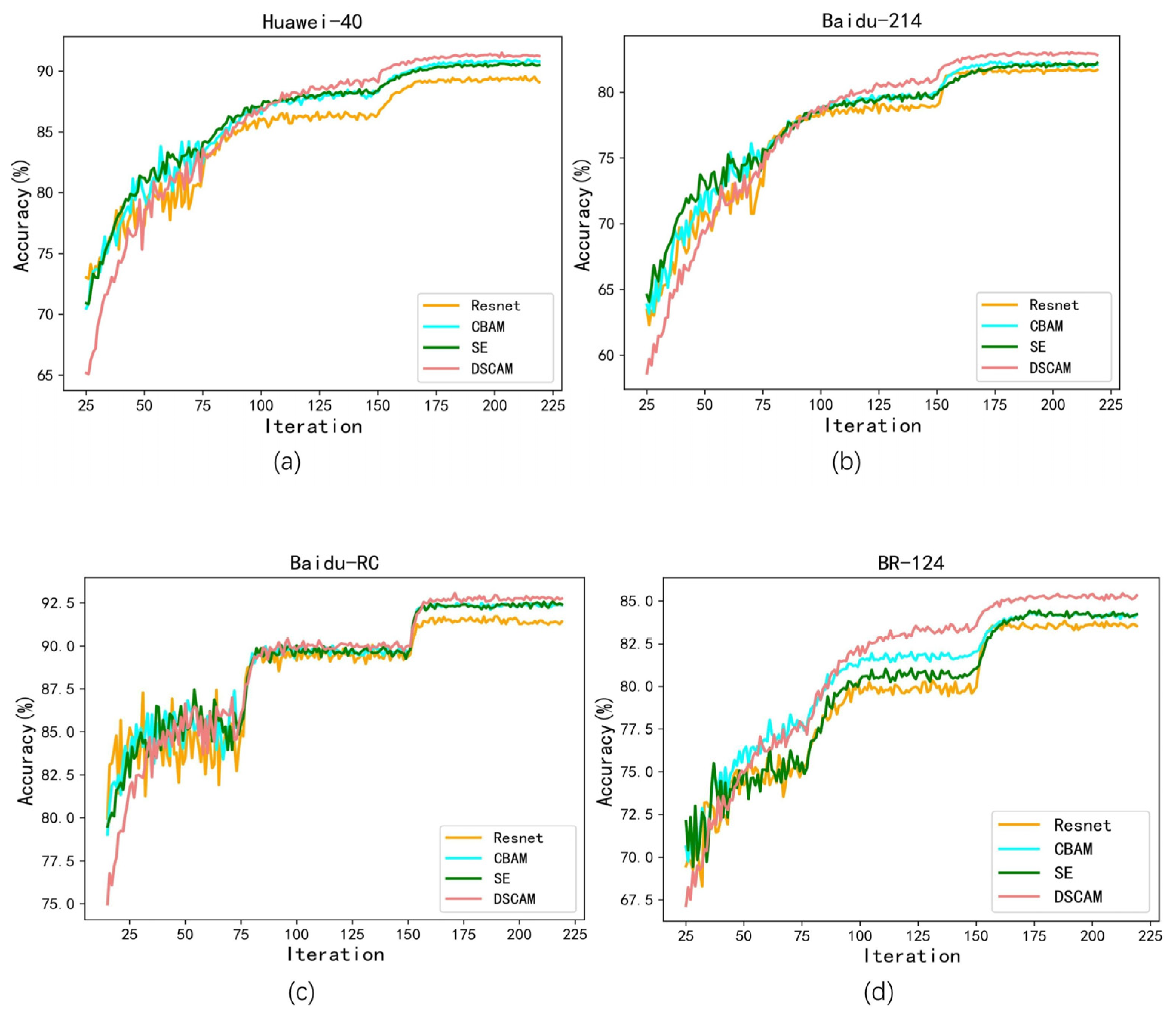
Figure 11 shows the accuracy curve of each method from Table 3. In the early stage of iterations, since the parameters in all networks are randomly initialized, their classification results are all very bad. Thus, we only show the accuracy curves between the 25th to 225th training iterations of different methods in this figure. It can be found that the accuracy of our method is lower than other methods when the number of training iterations is small, which may be due to our DSCAM containing more convolution operations. Moreover, since we initially set a larger learning rate to ensure that the networks can quickly achieve a high accuracy at the beginning, the fluctuant phenomena can be clearly seen from the accuracy curves of different methods at the early training stage. Nevertheless, after the learning rate is reduced at the 75th and 150th training iterations, the fluctuation of accuracy curves obtained by all methods become small and the performance of our method improves rapidly and gradually surpasses other approaches with the increasing of training iterations. At last, we can also observe that the average accuracy of all methods becomes nearly stable after 200 iterations, so the classification accuracy at the 200th training iteration is taken as the final experimental result in Table 3.

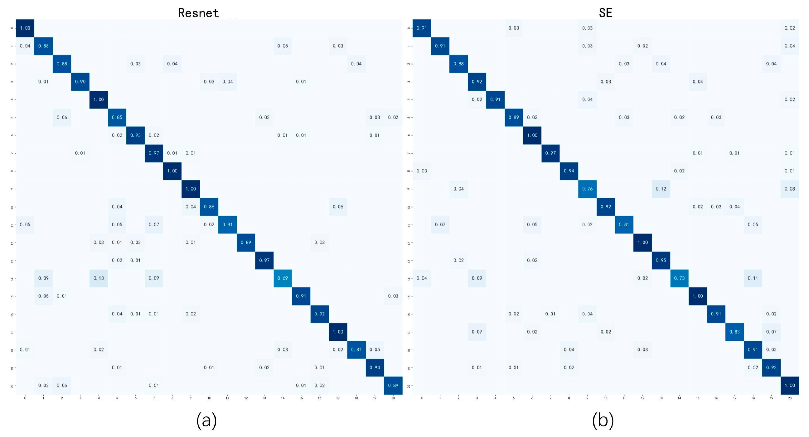
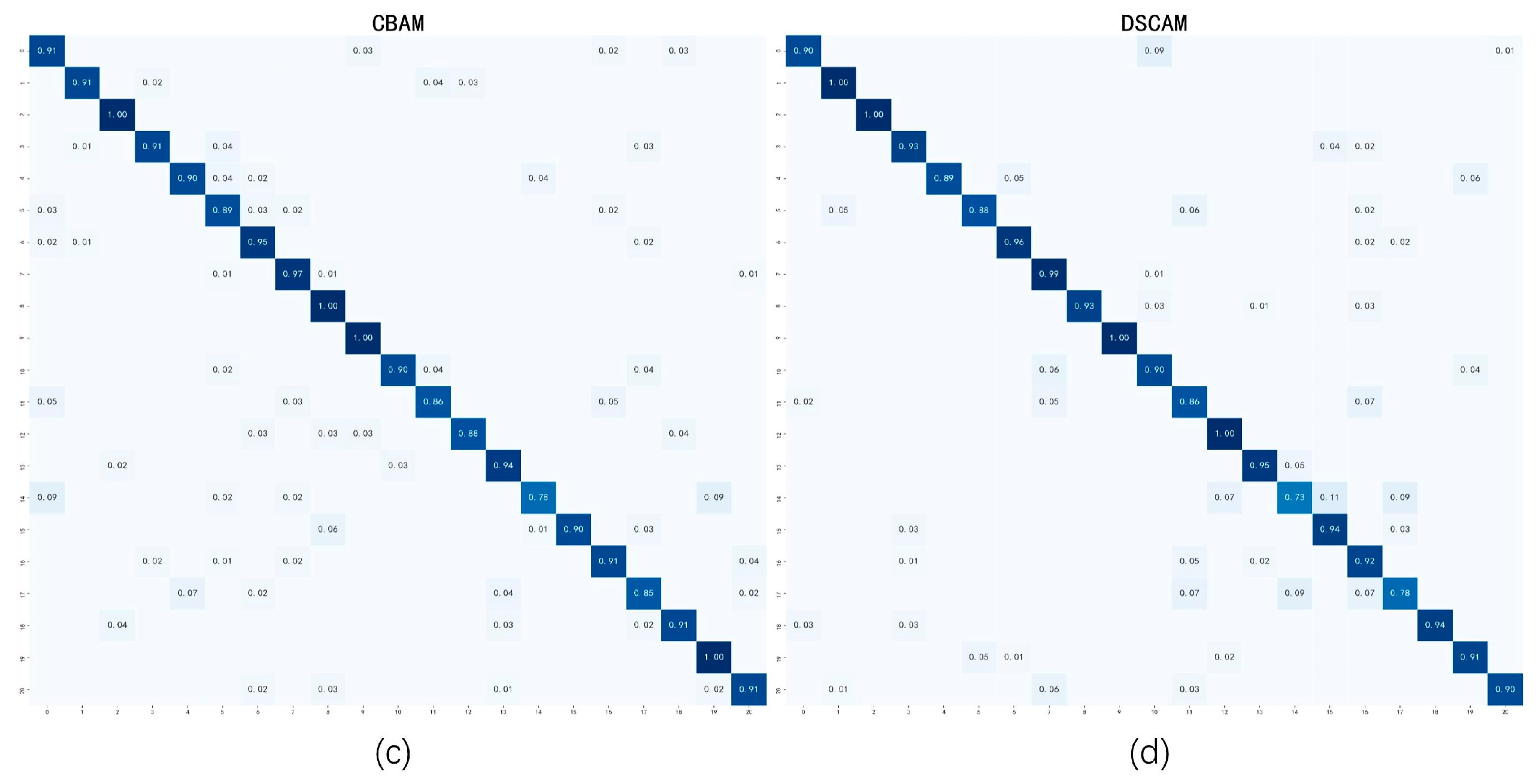
Next, the confusion matrices of accuracy obtained by various methods on the Baidu-RC dataset are provided for comparison. The confusion matrix can reflect the classification accuracy of each class. The diagonal of the confusion matrix represents the accuracy of each class, and the off-diagonal elements indicate the degree of misclassification. From Figure 12, it can be seen that the confusion matrix obtained by our method is sparser than other methods, which means that our method can extract more discriminative features and classify fewer garbage images into incorrect categories.

To test the statistical significance between different models, the McNemar–Bowker test [38], which can analyze the classification outcome of more than two classes is employed. In our experiment, the significant level is set as 0.05.

Table 4. McNemar–Bowker test between DSCAM and compared methods.

Dataset	DSCAM & Resnet	DSCAM & CBAM	DSCAM & SE
Huawei-40	p = 0.0205	p = 0.0362	p = 0.0275
Baidu-214	p = 0.0136	p = 0.0188	p = 0.0166
Baidu-RC	p = 0.0435	p = 0.0491	p = 0.0494
BR-124	p = 0.0065	p = 0.0183	p = 0.0155

demonstrates the results (p-value) of the McNemar–Bowker test between our DSCAM and compared methods. From these results, we can find that the p-values are all smaller than the significant level. Therefore, through comprehensively considering the results in Table 4, Figure 11 and Figure 12, we can see that the performance of our DSCAM is significantly superior to other methods.

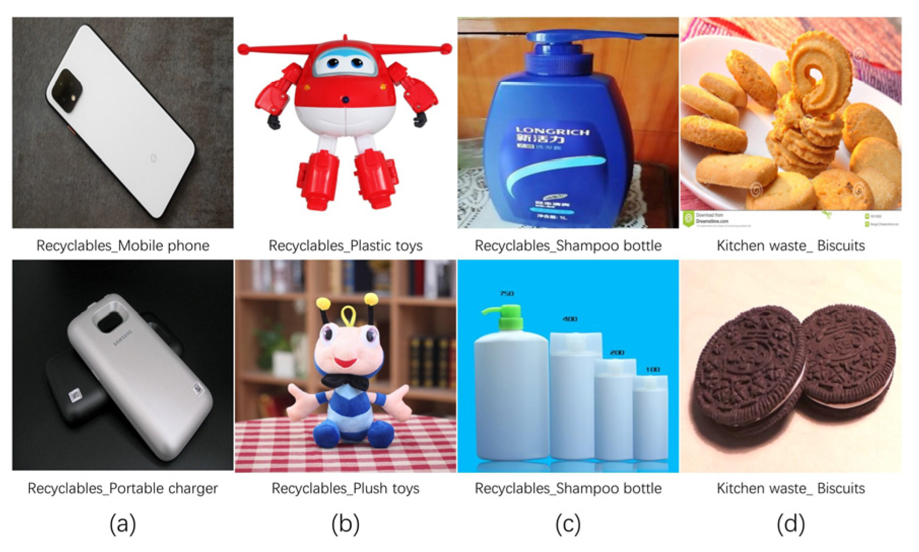
To illustrate that DSCAM can effectively deal with the inter-class similarity and intra-class variance problem, we demonstrate some images in Figure 13, which misclassified by comparison methods (i.e., Resnet, SE, CBAM) but correctly classified by our method. In this figure, the garbage images in columns (a) and (b) are from different classes. Nevertheless, since the two images in the same column exhibit similar appearances, it is difficult to distinguish them. Contrarily, the garbage images in columns (c) and (d) come from the same class but have quite different appearances. Thus, they are also easily misclassified. However, with the help of the Resnet architecture, the attention module and depth separable convolution, the proposed DSCAM can capture more discriminative deep features and neglect the irrelevant information in the image. Thus, the images in Figure 13 are correctly classified to their corresponding categories by our method. This means that our DSCAM can address the limitations of other methods to some extent.

4.4. Parameter Sensitivity

There exist some parameters whose values may influence the performance of our proposed DSCAM. Thus, we conducted some experiments to test the sensitivity of our method with these parameters.

First, the impact of the parameters (i.e., kernel size and reduction ratio) in depth-wise separable convolution on our DSCAM is evaluated. The performances of our method under various parameter values can be seen in

Table 5. Classification accuracy (%) with different parameter values in depth-wise separable convolution.

Depth Convolution Size and Reduction Ratio	Huawei-40	Baidu-214	Baidu-RC	BR-124
3 × 3 (r = 8)	91.02	82.66	92.53	84.78
3 × 3 (r = 16)	91.20	83.01	92.77	85.35
3 × 3 (r = 32)	89.90	81.87	91.65	83.86
5 × 5 (r = 8)	90.35	82.47	92.03	83.87
5 × 5 (r = 16)	90.76	82.70	92.36	84.21
5 × 5 (r = 32)	89.63	81.25	91.42	83.01
7 × 7 (r = 8)	89.92	81.86	91.76	83.43
7 × 7 (r = 16)	90.25	82.01	91.95	83.89
7 × 7 (r = 32)	89.03	80.57	91.06	82.62

. From this table, it can be found that DSCAM achieves its best classification accuracy when the kernel size and reduction ratio are set as $3\times 3$ and $r=16$. The reason may be that a large kernel size will enlarge the receptive field, which overlooks the detailed fine feature in the image. Besides, the purpose of the reduction ratio is to control the degree of information compression along channels. Thus, a larger reduction ratio will lose some useful information, and a smaller reduction ratio will cause information redundancy.

Since spatial and channel attention have different processes and functions, the order of them may affect the overall performance of our method. Therefore, we compare three different ways of arranging the channel and spatial attention modules: sequential channel+spatial (C + S), sequential spatial+channel (S + C), and parallel use both attention modules (S&C). From the comparison result in

Table 6. Classification accuracy (%) in different architecture combinations of our methods.

Architecture	Huawei-40	Baidu-214	Baidu-RC	BR-124
C + S	91.20	83.01	92.77	85.35
S + C	90.17	81.84	92.30	84.21
S&C	89.92	80.24	91.75	83.60

, we can see that sequentially generating the attention maps outperforms the parallel manner. Furthermore, the channel-first order performs slightly better than the spatial-first order. This result justifies the design of our network architecture in Figure 3.

4.5. Ablation Study

The depth of a network (i.e., the number of layers in a network) is an important factor to affect its performance. Generally, more layers will make the network obtain high accuracy. But more layers are also accompanied by more parameters, which would bring longer training and test time. Here, we conduct some experiments to justify the rationality of Resnet-50 as the backbone of our network.

First, we replace the backbone of our network with deeper Resnet-101 and Resnet-152. From the experimental results in

Table 7. Comparison of different backbone networks on the Huawei-40 dataset.

Backbone	Accuracy	Training/Test Time Per Image	Params Size (MB)	Memory Size (MB)
DSCAM + Resnet-101	91.27	0.150/0.060	198.90	835.35
DSCAM + Resnet-152	91.32	0.220/0.075	272.71	1183.20
DSCAM + Densenet-121	91.30	0.242/0.088	31.91	5589.45
DSCAM + Densenet-169	91.35	0.278/0.102	53.25	6847.50
DSCAM + Resnet-50	91.20	0.081/0.048	109.30	523.79

, it can be seen that the backbone network with more layers can slightly improve the performance of our method from 91.20% to 91.27% (Resnet-101) and 91.32% (Resnet-152). However, Resnet-101 and Resnet-152 also greatly increase the number of parameters, training/test time and GPU memory size. Then, we also employ Densenet-121 and Densenet-169 [28] as the backbone of our network. From Table 7, it can also be found that the Densenets with more layers achieve better performance than Resnet-50. Nevertheless, although Densenet-121 and Densenet-169 outperform Resnet-101 and Resnet-152 with fewer parameters, they require larger GPU memory sizes due to the massive concatenation operations in them. Besides, Densenet also needs more training/test time due to it uses many small convolutions in the network, which runs slower on a GPU than large compact convolutions with the same number of GFLOPS [39]. At last, through taking all factors (such as accuracy, time, number of parameters and memory size) into consideration, we choose Resnet-50 as the backbone of our network since it could obtain comparable garbage classification accuracy without very large computation and memory consumption.

4.6. Real Scene Application

In order to test the classification result of the proposed DSCAM in real scenes, we construct a simple real garbage dataset. As mentioned before, recyclable garbage is very valuable in real life. Therefore, 400 recyclable garbage images with 20 categories (20 images per category) in real scenes are collected through taking pictures and an online search. Some samples of this dataset are shown in Figure 14. At the same time, to enrich the amount of data, the images in the dataset are randomly clipped, rotated and filled with background for data augmentation. As a result, a total of 2000 recyclable garbage images (100 images per category) were obtained.

In this experiment, we directly inputted the collected garbage images to different networks pre-trained on the BR-124 dataset.

Table 8. Classification accuracy (%) obtained by different methods on the Real Scene dataset.

Methods	Real Scene Dataset
VGG-19	91.0
Xception	92.5
X-DenseNet	95.6
MobileNet-V3	98.5
GNet	98.2
Resnet	97.6
SE	98.0
CBAM	98.7
DSCAM	98.9

shows the classification result obtained by each network. First, it can be seen that VGG-19 and Xception obtain the worst accuracy among all methods. Second, the performances of X-DenseNet and Resnet are inferior to other models with an attention mechanism, such as SE, MobileNet-V3, GNet and CBAM. At last, the proposed DSCAM achieved the best results. The observations in Table 8 are consistent with those in the previous experiments, which shows our method has good generalization and can effectively deal with the garbage images in real scenes.

5. Conclusions

In this paper, we focus on developing a specific deep CNN for garbage image classification problems. To this end, we proposed the attention module DSCAM, which provides a novel mechanism to construct attention weights. Unlike the original attention mechanism, which only uses a pooling layer to infer correlations in channels and spatial, DSCAM utilizes depth-wise separable convolutions to construct the inherent relationship of channel and spatial, which can make the network obtain more discriminative features. Moreover, a Resnet-50 with more convolutional layers is also adopted as the backbone of our method, so that its classification ability can be further improved. Several experiments were conducted to evaluate our method on five garbage datasets. The experimental results illustrate that our method achieves better performance than the compared methods.

In the future, we will embed our attention modules into more recent proposed backbone networks (such as visual transformer [40]) to test their performance on garbage image classification. Furthermore, combining the proposed DSCAM with some hardware and devices (such as a robot chassis, a robotic arm and a camera) to create an automatic garbage sorting system is another interesting topic for future study.