The Interactive Relationships between the Tourism-Transportation-Ecological Environment System of Provinces along the ‘Silk Road Economic Belt’ in China

Abstract

Taking nine provinces and cities along the ‘Silk Road Economic Belt’ as an example, this paper constructs an evaluation index system of the coupling coordination degree of the tourism–transportation–ecological environment system (TTE system), analyzes the spatial–temporal evolution and regional differences of the coupling coordination level of the TTE system from 2004 to 2016 using the mean square error index model and the scissor difference model, and uses the EKC curve model to further verify the interactive relationship between the tourism economy and the ecological environment. The results show the following. (1) The comprehensive evaluation values of the tourism subsystem and transportation subsystem are on an overall upward trend and the comprehensive evaluation value of the ecological environment subsystem is in constant flux. (2) The coupling coordination degree of the TTE system generally develops in a good coordination direction, but the conversion rate of the coupling coordination degree of each province is different. (3) Regarding the north–south region divergence, the degree of coupling and coordination within the region is “strong in the south and weak in the north”. (4) The tourism subsystem and the transportation subsystem are interdependent and mutually restrictive. (5) There is a strong correlation between tourism, economic growth, and environmental quality, but in most provinces, the relationship between them does not accord with the inverted U-shaped environmental Kuznets curve.

1. Introduction

Building the Silk Road Economic Belt was a significant initiative, which was proposed by President Xi Jinping during his visit to Central and Southeast Asian countries in 2013. In order to promote the effective implementation of this strategy, China will cultivate new economic growth poles on the Silk Road Economic Belt by introducing industries and gathering the population. The implementation of the ‘One Belt, One Road’ initiative is conducive to the fast development of the provinces along the western route, and it creates rare opportunities for tourism development, cultural dissemination, and infrastructure construction in the central and western provinces. However, due to the current situation, the development of provinces along the Silk Road Economic Belt in China has the following problems: administrative barriers between provinces still exist, the radiation driving ability of central cities is insufficient, and the traffic accessibility between provincial capitals is inadequate; the ecological environment has relatively deteriorated, and the government is faced with the problems of carbon emission and watershed water pollution prevention and control. Regional industrial transfer and interest coordination mechanisms need to be improved, and barrier-free tourism zones still need to be implemented. Therefore, exploring the coupling and coordinated development of the tourism system, transportation system, and ecological environment system of provinces along the Silk Road Economic Belt is necessary to promote the integration process of these provinces, which is an important measure to boost the implementation of the western development strategy, and it is an important driving force to accelerate the west and central provinces to become the new supports of China’s economy.

Since entering the new century, the tourism industry has gradually become one of the most vigorous industries in the world’s economic activities. Among the many characteristics of tourism activities, the element characteristic of long distance determines that tourists need to use transportation to complete tourism activities. With the successful development of the tourism economy and the improvement of transportation networks, the relationship between the tourism economy and transportation development has gradually become a heated issue in academic research. However, the environmental dependence of tourism and the resource consumption of the transportation industry determine that there is a complex and unified relationship between the tourism economy, transportation development, and the ecological environment that restrict and promote each other.

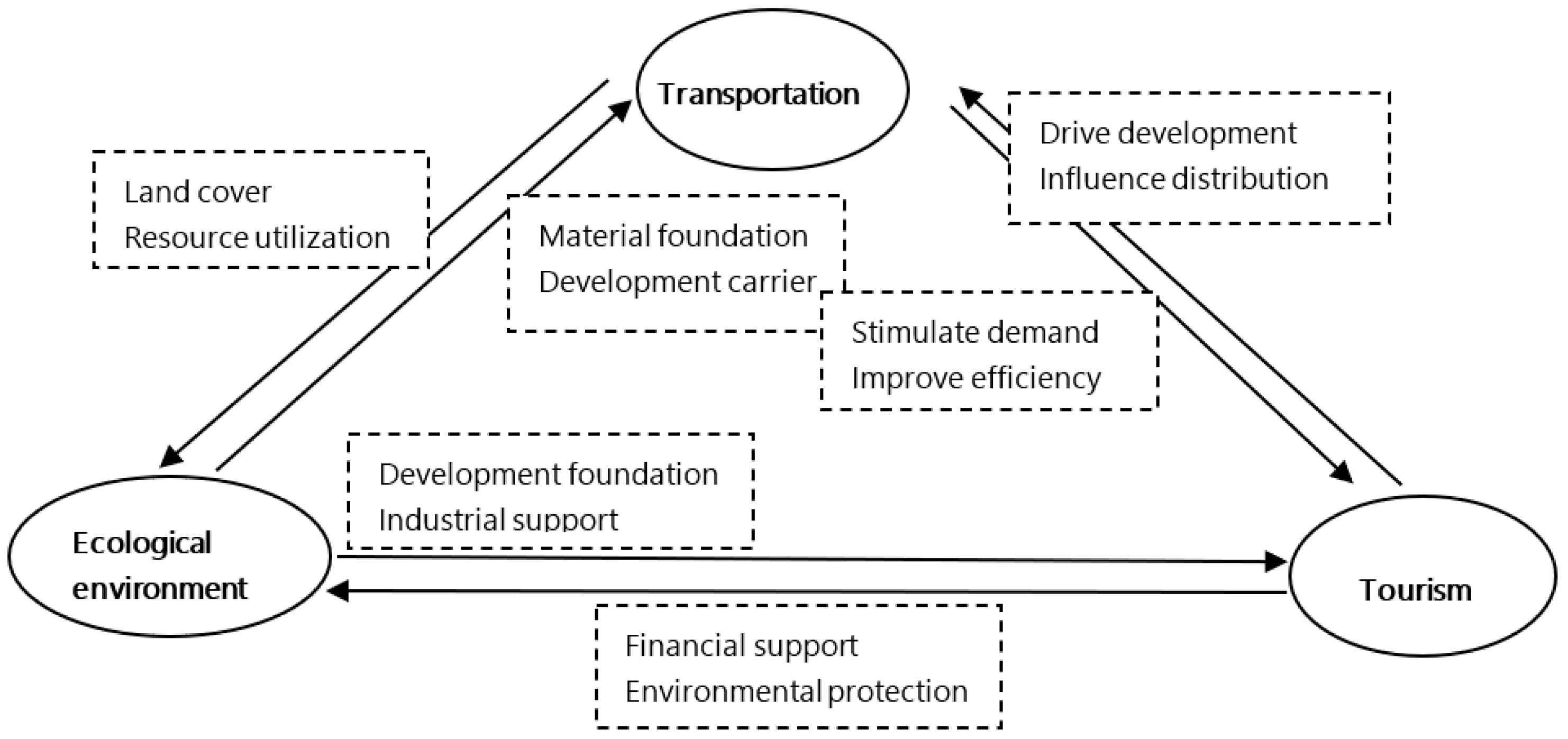
The TTE system, which is a vast open system with complex content and a diversified structure, has the following coupling characteristics (The interaction relationship of the three subsystems in the TTE system is shown in Figure 1).

Firstly, the ecological environment is an essential carrier on which the tourism and transportation industries carry out activities. On the one hand, the development of the tourism industry depends on the ecological environment. A good ecological environment can improve the experience and satisfaction of tourists and promote the sustainable and healthy development of the tourism economy. On the other hand, if the ecological environment is destroyed, the impact on traffic is undeniable. For example, natural disasters such as debris flow, sandstorms, and mountain landslides will reduce traffic safety and transportation efficiency, thus causing an increase in traffic operation costs.

Secondly, tourism development can guarantee the outcome of transportation and improve the ecological environment. Growth in tourism demand will stimulate the construction and expansion of transport infrastructure, and it can affect the evolution of transport network space–time patterns. In addition, the development of tourism should be based on not exceeding the carrying capacity of the local ecological environment. It can promote the improvement of the regional environment by providing funds and science and technology through the economic benefits generated by tourism.

Finally, the construction of transportation infrastructure effectively promotes the development of tourism and the protection of the ecological environment. Traffic can connect tourist sources and destinations, and regional traffic plays a crucial role in developing tourism economic activities. If transportation construction is blindly designed at the cost of the ecological environment, it will cause environmental problems such as vegetation degradation, species extinction, and resource waste.

At present, domestic and foreign scholars have studied the interaction between tourism and the ecological environment and tourism and transportation, and most of them focus on the perspective of binary relationships: the impact of tourism activities on the ecological environment, the coordinated development between transport and the tourism economy, and the effect of the ecological environment on tourism.

(1)

Transportation, which is one of the three pillars of tourism, is a prerequisite for people to carry out tourism activities, the premise and material basis for tourism development, and the critical lifeblood of tourism development. In recent years, with traffic system upgrades, regions formed by highways, high-speed railways, civil aviation, and urban rail transits as the main body of the integrated operation of the system improve tourism between tourists and destination accessibility, shorten the residents’ travel time, and to some extent, deepen the correlation between the regional tourism industry; there are also new requirements for the spatial allocation of tourism resources. Jaarsma’s (2008) research on rural tourism found that traffic congestion has seriously affected the travel experience of leisure tourists. When formulating a traffic management plan, it is necessary to fully consider the area’s recreational uses and the interdependence of the actors involved [1]. Houts et al. (2013) believes that although other tourist facilities have promoted the large-scale development of the tourism industry, the development of the air transportation industry has taken the tourism industry one giant step forward [2]. Carolina et al. (2015) performed research in Brazil to study the interactive relationship between tourism and transportation, and they proposed new research methods [3]. Alkheder et al. (2015) analyzed and evaluated the conditions of the existing transportation system of Ajloun, Jordan, and its contributions to the sustainable development of the country’s tourism industry, and they proposed that Jordan should fully consider its transportation industry planning when formulating tourism planning [4]. Sharkhuu et al. (2020) argue that good infrastructure and excellent road network accessibility are crucial drivers of development in all sectors of the economy. The gravity model is used to conduct an empirical study on international tourists arriving in Mongolia. The influence of classic demand factors, such as transportation infrastructure and carbon dioxide emissions on Mongolian tourism flows, is expounded [5]. Wang et al. (2021) evaluated tourism efficiency and transport accessibility from 2011 to 2017 by taking 17 administrative units in Hubei Province as research objects. The results show that the spatial matching and coupling degree between tourism efficiency and transport accessibility should be upgraded to improve the sustainability of tourism development [6]. By comparing Bihor-Hajdú–Bihar and Maramures–Zakarpattya cross-border regions, Wendt et al. (2021) analyzed leading tourism indicators and studied the progress made in transportation infrastructure driven by tourism to determine whether there is a correlation between the development of transportation networks and the increase in tourist traffic [7]. Papatheodorou’s (2021) research, based on microeconomics and economic geography tools, highlights the implications of air transport accessibility for tourism development. Utilizing synergy on synergies and revitalizing air transportation and tourism in the post-commercial environment of COVID-19 has added value, which is conducive to promoting the development of transportation and tourism [8]. The interactive relationship between tourism and transportation in the paper is improved. Through the literature review of the transportation system and tourism system, it can be seen that current research on the interaction between the two systems has both qualitative and quantitative analysis, but the evaluation method is relatively singular, which will inevitably bring research limitations. In addition, there are few studies on the interactive relationship between the transportation system and tourism system in the Silk Road Economic Belt region. The research objects of this paper are the provinces and cities along the Silk Road Economic Belt in China, and the evaluation methods of the combination of entropy weight method and cosine theorem are adopted, so the conclusions have more reference value.

(2)

Although tourism development can bring economic benefits to a region, it is crucial to consider the long-term impact of tourism on a particular area, especially on the premise that tourism depends on a specific ecological environment and the long-term effect of extensive development of tourism on the ecological environment. Hill et al. (2006) found that tourism activities interfere with the survival and reproduction of certain species on Mount Kosciuszko in Australia [9]. Burgin et al. (2011) found that yachting activities in coastal waters will affect the physics, chemistry, and biology of the ocean ecosystem [10]. Taking Harbin as an example, Xuan et al. (2013) created a mathematical model in 2010 to analyze the coordinated development relationship between Harbin’s tourism economy and the ecological environment, and they proposed policies and measures to promote the coordinated development of tourism and the ecological environment [11]. Huang et al. (2013) believes that the increase in the number of tourists and the mismanagement of natural resources has caused severe damage to the ecological environment. Huang constructed an ecological security evaluation system for the scenic area of the island city in the Hunan Province and provided a model example for the sustainable development of island tourism [12]. Gon et al. (2016) pointed out that the yacht tourism industry has resulted in negative environmental impacts, such as increased marine and coastal waste, increased sea pollution, and more crowded beaches on the Italian coastal cities of Grado and Lignan [13]. Zhong et al. (2020) studied the reserve as a kind of recreation ecology and the relationship between the contradiction of ecological protection, analyzing the historical development process of recreation ecology tourism destinations in China, focusing on the impact of tourism on the natural environment, the environmental management of tourism, and the different types of sustainable tourism in the development of the tourism destination [14]. Yong et al. (2021) collected data from 48 developing countries across Africa, Asia, and South America to determine the extent to which people’s awareness of environmental protection is at odds with ecological damage during tourism and to provide new insights into mitigating sea-level rise and promoting tourism [15]. From the above literature review, it can be seen that the research results of scholars domestically and abroad on tourism systems and ecological environment protection are relatively affluent, but the research perspective still regards the tourism system and the ecological environment system as two separate systems to explain the impact of one system on another. The contribution of this paper to the existing literature is to build a TTE system including the transportation system, tourism system, and ecological environment system. It not only studies the interactive relationship between the ecological environment system and tourism system but also studies the role of the tourism system and ecological environment protection system in the coordinated development of a TTE system. In addition, the interaction between specific tourism system evaluation indicators and ecological environment protection indicators is also studied through the EKC model.

(3)

It is important to conduct an interaction study of the transportation system and ecological environment system. Along with the development of transportation construction, the local ecosystem will be affected accordingly. There will be certain risks to water resources, land resources, forest resources, and other dependent aspects. Daigle et al. (2010) analyzed the impact of unpaved roads in Colombia on land, vegetation, and wildlife and argued that proper planning should be adopted to reduce the negative effect of paved roads [16]. Zhou et al. (2011) took the integrated transportation system and the ecological environment system as the research objects and analyzed the interactive relationship between the integrated transportation system and the ecological environment system by using the game model and analyzing the factors that affect the sustainable development of integrated transportation [17]. Zhou et al. (2012) believed that with the emergence of new transportation concepts and the development of advanced transportation methods, the construction of comprehensive transportation must meet the principles of ecology planning, reduce resource and energy consumption, reduce environmental pollution, and promote the harmonious development of the transportation industry and the environment [18]. Sun et al. (2015) believes that carbon dioxide emissions are the leading cause of global warming. The implementation of environmentally friendly regional transportation is essential to promote the sustainability of the tourism industry. Based on this idea, a model for estimating carbon dioxide emissions from regional tourism transportation was constructed and erected [19]. Ma et al. (2008) analyzed the interaction between energy consumption and environmental pollution in transport and discussed the social and economic benefits of energy conservation and emission reduction [20]. Wang et al. (2019) studied the positive impact of transportation activities such as tourist roads on ecology, entertainment, culture, and education while bringing tourism value to scenic spots [21]. Li et al. (2020) point out that a range of transport policies are used in both developed and developing countries to seek ways to mitigate pollution, showing that transport policies have significant and lasting impacts on urban life and global climate change [22]. Through the literature review of the transportation system and ecological environment protection, it can be seen that the current research mainly expounds on the relationship between the transportation facilities’ construction and ecological environment protection through qualitative methods. The contribution of this paper to the existing literature is to establish a comprehensive evaluation index system of the transportation system and ecosystem and quantitatively study the interactive relationship between the provinces and cities along the Silk Road Economic Belt from 2004 to 2016 by using a variety of methods. By analyzing the critical evaluation indexes, we can find a way to improve the benign interaction between the transportation system and ecological environment protection.

(4)

As a brief literature summary, domestic and foreign scholars who study the tourism system, the transport system, and the ecological environment system in a single system or a dual system in this field of research enrich the theory of this paper and provide valuable references. Nevertheless, the evaluation index selection lacks consideration, and the evaluation system is a little rough and straightforward, which cannot accurately and reasonably reflect the development of the TTE system. In the determination of index weight, a single subjective weight method or single objective weight method makes the weight have an inevitable defect. Most of the research on coordination evaluation is limited to static coordination assessment degree, and few studies use the scissors difference model to further analyze its dynamic evolution characteristics. In related studies, few scholars use the mean square error index model to study the spatiotemporal characteristics of coupling coordination degree.

This paper establishes a comprehensive evaluation index system of the TTE system. The objective weight of each evaluation index under different methods is determined by the law of cosine and entropy weight. The comprehensive weight of each evaluation index is determined by the combination weighting method of game theory. Based on this, the comprehensive evaluation value of each sample is calculated; this value is used to judge the pros and cons of the evaluation object. Second, the coupling coordination degree model and the scissors model are used to dynamically analyze the time evolution of the coupling coordination degree among the tourism system, the transportation system, and the ecological environment system of the nine provinces along the Silk Road Economic Belt from 2004 to 2016. Then, the provinces are divided by the coupling coordination degree to analyze interprovincial and north–south differences. Finally, using the interactive relationship between the tourism system and transportation system, tourism economic development and environmental quality are analyzed using the scissors model and the Kuznets curve. The analysis results provide a valuable and scientific basis for the relevant entities to formulate coordinated development strategies. It can be seen that to a certain extent, the research in this paper makes up for the gap in previous studies.

Compared with the existing literature, the possible innovations of this paper are as follows:

(1)

Most scholars use a single system or double system to measure the coupling degree and coupling coordination degree. In this paper, based on the current research results of coupling coordination and the actual development of nine provinces along the Silk Road Economic Belt, an evaluation index system of coupling coordination degree of the TTE system consisting of three subsystems is established.

(2)

This paper uses the method of entropy weight, the law of cosines, the combination weighting method in game theory, the coupling coordination degree model, and the scissors model along with the Silk Road Economic Belt province of the TTE system coupling and coupling coordination degree of measurement. Through the mean square deviation index model, this paper delves into nine provinces using the coupling coordination degree of regional differences and north–south differences. The results show the temporal and spatial characteristics of coupling coordination degree, and they show its temporal variation and spatial evolution more directly.

(3)

This paper not only confirms the rising trend of the coupling coordination degree of the TTE system in the Silk Road Economic Belt and the unbalanced spatial pattern of its distribution but also further explores the interactive relationship between tourism, economic development, and the ecological environment by using the EKC model.

Theoretical significance:

(1)

Having perfected the subsystems of travel, the transportation subsystem, and the ecological index evaluation system simultaneously to overcome the defects of the single evaluation method, this paper uses the method of cosine theorem and the entropy weight method to determine the objective weight of each evaluation index. Each index was determined by the method of game theory combination empowerment of combination weight, making the three subsystems of comprehensive evaluation more accurate.

(2)

The coupling coordination degree of each subsystem is elaborated, and the theoretical framework of the TTE system is perfected. Before the study of an area along with the province, primary consideration for a single subsystem (traffic system, tourism system, and ecosystem) or of the interactions between two subsystems will expand the research to three systems; this paper established the TTE integration system, which is a comprehensive study of the complex coupling relationship between the three subsystems.

Practical significance:

(1)

The construction of the ‘Belt and Road’ initiative is an important measure to expand China’s all-around opening up under the new situation, which is conducive to more countries sharing development opportunities and achievements. The development of tourism, transportation, construction, and the improvement of the environment to promote the implementation of the area play an important role. Still, there are inevitable provinces along the Silk Road Economic Belt with weak infrastructure, destroyed ecological environment, and stumbling problems in tourism development; because of this study, promoting the coordinated development of the TTE system and measures has practical significance.

(2)

The implementation of the economic development strategy along the Belt and Road provides a relatively loose external environment and good opportunities for the old industrial base of northeast China. The conclusions of this study also have specific guiding significance for the revitalization of the old northeast industrial base.

The sections of this study are arranged as follows: the first section is the introduction and related literature review; the second section introduces the materials and methods of this study and describes the research area, evaluation index system, data sources, and data preprocessing; the third section discusses the results and related explanations; the fourth section presents the research conclusions and policy recommendations.

2. Materials and Methods

2.1. Study Area

At the end of 2017, the nine provinces along the Silk Road Economic Belt accounted for 16.92% of China’s total economic output. These nine provinces have rich natural and cultural resources, allowing their tourism industries to grow significantly. Among them, Shaanxi, Sichuan, Yunnan, Guangxi, and Xinjiang have huge tourism industries with abundant tourism resources, and they are in leading positions in national tourism development compared to the other provinces. Strong economic growth and reliable transportation networks can enable tourism development in Chongqing, Gansu, Qinghai, and Ningxia to maximize their significant late-comer advantages and huge development potential. In addition, transportation in these provinces has developed rapidly, and the operating mileage of various modes of transportation and the turnover of tourism have been increasing. In 2014, President Xi Jinping proposed that the Silk Road Economic Belt should realize the “five links” of policy, currency, roads, trade, and people’s hearts. Road connectivity is the key to realizing these five links. Countries and domestic provinces along the route have actively responded to the One Belt, One Road initiative and have increased the construction of transportation infrastructure. However, the development of the nine provinces along the route is not without its challenges, as the ecology outlook is not optimistic. According to the China Environmental Statistics Yearbook, in 2017, the wastewater discharge of the nine provinces along the route was 13.46 billion tons. Furthermore, the early tourism development and transportation infrastructure construction occurred too quickly at a large scale and without consideration for protecting the ecological environment. Serious problems, such as environmental pollution, environmental degradation, and resource depletion, have gradually become prominent.

2.2. Evaluation Index System and Data Sources

For the setting of indicators, scholars have different views. Shu et al. (2015) evaluated the tourism system with four grade 1 indicators, including tourism effect, tourism income, tourism employment, and tourism industry, and 10 grade 2 indicators. The evaluation indexes of an ecosystem include the population index, economic index, social index, cultural index, and ecological environment index, which are 5 grade 1 indexes and 27 grade 2 indexes [23]. Fei et al. (2021) built the evaluation indexes for the economic system, including the economic development scale and social and economic construction; evaluation indexes for the ecosystem include environmental pollution status and effectiveness of environmental management, and evaluation indexes for the tourism system include tourism market size and tourism factor structure [24]. Han et al. (2021) evaluated the economic systems, including economic aggregate, economic benefits, and economic structure, and they assessed the environmental systems, including environmental quality and environmental governance [25]. Tang et al. (2015) evaluated the tourism system by developing scale and economic benefits, and they assessed the ecosystem by ecological quality, resource consumption, and environmental protection [26]. Wu et al. (2019) evaluated the transportation system, including infrastructure construction, transportation service, and transportation efficiency. They evaluated the tourism system including tourism industry scale, tourism industry benefit, and tourism service [27].

Based on the availability of data, the representativeness of indicators, the comprehensiveness of evaluation, and the existing research, this paper closely focuses on six dimensions, including scale, conditions, scale efficiency, status, pressure, and response, and it selects 27 evaluation indicators to construct an evaluation index of the TTE system (

Table 1. Evaluation index system of the TTE system.

Subsystem	Criterion	Index	Unit	Effect
Tourism system	scale	Number of domestic tourists	Million people	Positive
		Domestic tourism income	100 million yuan	Positive
		Number of inbound tourists	Million people	Positive
		Inbound tourism income	Ten thousand dollars	Positive
	conditions	Number of employees in catering industry	People	Positive
		Number of employees in accommodation industry	People	Positive
		The proportion of total tourism revenue to GDP	%	Positive
		The proportion of domestic tourists in the population	%	Positive
		Private passenger car ownership	Ten thousand	Positive
Transportation system	scale efficiency	Railway passenger traffic	Ten thousand people	Positive
		Highway passenger traffic	Ten thousand people	Positive
		Railway passenger turnover	Billion person-kilometers	Positive
		Highway passenger turnover	Billion person-kilometers	Positive
	conditions	Number of employees in the transportation industry	People	Positive
		Railway operating mileage	Million kilometers	Positive
		Highway mileage	Million kilometers	Positive
		High-speed grade highway mileage	Million kilometers	Positive
		Number of public transportation vehicles operated	Vehicles	Positive
Environmental system	status	Green coverage rate in built-up area	%	Positive
		Park green area per capita	M2/person	Positive
		Forest coverage	%	Positive
	pressure	Sulfur dioxide emissions	Tons	Negative
		Total wastewater discharge	Ten thousand tons	Negative
		Industrial solid waste generation	Ten thousand tons	Negative
	response	Harmless treatment rate of domestic garbage	%	Positive
		Industrial pollution control completed investment	Ten thousand yuan	Positive
		The daily treatment capacity of urban sewage	Ten thousand cubic meters

).

The data are sourced from the China Statistical Yearbook, the China Environment Statistical Yearbook, the China Tourism Statistical Yearbook, and the China City Statistical Yearbook, as well as other statistical yearbooks and national economic and social development statistical bulletins from 2004 to 2016.

2.3. Research Methods

2.3.1. Determination of Comprehensive Weight

Most prior studies adopt a single method to determine the weight of the evaluation index, which cannot overcome the shortcomings of using a single evaluation method. Therefore, this paper adopts the law of cosines and the entropy weighting method to determine the weight of each evaluation index; then, it calculates the comprehensive weight of each evaluation index through the combination weighting method of game theory.

The Law of Cosines

The cosine-included angle value, also known as the similarity, can objectively display the deviation degree of the distribution of each index value to better reflect the relative importance of each index. The specific steps are as follows (Xu et al., 2017) [28].

(1)

Construct the optimal solution vector $L_i^{+}$ and the worst solution vector $L_i^{-}$ of the evaluation index

$$L_i^{+}\{\begin{array}{c}\underset{1\le j\le n}{\max }\left\{S_{ij}\right\},i\in I_1\\ \underset{1\le j\le n}{\mathrm{mix}}\left\{S_{ij}\right\},i\in I_2\end{array}$$

(1)

$$L_i^{-}\{\begin{array}{c}\underset{1\le j\le n}{\mathrm{mix}}\left\{S_{ij}\right\},i\in I_1\\ \underset{1\le j\le n}{\max }\left\{S_{ij}\right\},i\in I_2\end{array}$$

(2)

where $L_i^{+}$ and $L_i^{-}$ represent the best value and worst value of each evaluation index, respectively; $S_{ij}$ represents the index evaluation value of the $i$ index in year $j$; $I_1$ and $I_2$ represent the positive effect index set (benefit index set) and the negative effect index set (cost index set), respectively; and $n$ represents the number of index evaluations.

(2)

Use the range method to establish the relative deviation matrix between each evaluation plan and the optimal solution vector and the worst solution vector:

$${\left(r_{ij}\right)}_{m\times n}={\left(\frac{\left|S_{ij}-L_i^{+}\right|}{\underset{1\le j\le n}{\max }\left\{S_{ij}\right\}-\underset{1\le j\le n}{\mathrm{mix}}\left\{S_{ij}\right\}}\right)}_{m\times n}$$

(3)

$${\left(t_{ij}\right)}_{m\times n}={\left(\frac{\left|S_{ij}-L_i^{-}\right|}{\underset{1\le j\le n}{\max }\left\{S_{ij}\right\}-\underset{1\le j\le n}{\mathrm{mix}}\left\{S_{ij}\right\}}\right)}_{m\times n}$$

(4)

where ${\left(r_{ij}\right)}_{m\times n}$ represents the relative deviation matrix between each evaluation plan and the optimal solution vector; ${\left(t_{ij}\right)}_{m\times n}$ represents the relative deviation matrix of each evaluation plan and the worst solution vector; $r_{ij}$ represents the degree of deviation between $S_{ij}$ and the absolute value of the optimal value $L_i^{+}$ relative to the range; and $t_{ij}$ represents the degree of deviation between $S_{ij}$ and the absolute value of the worst value $L_i^{-}$ relative to the range.

(3)

Determine the cosine-included angle value of the index:

$$c_i=cos{r}_i,t_i=\frac{{{\displaystyle \sum }}_{j=1}^n{r}_{ij\times }{t}_{ij}}{\sqrt{{{\displaystyle \sum }}_{j=1}^n{\left(t_{ij}\right)}^2}\sqrt{{{\displaystyle \sum }}_{j=1}^n{\left(r_{ij}\right)}^2}}$$

(5)

where $c_i$ represents the cosine-included angle value between the optimal deviation matrix row vector $r_{ij}$ and the worst deviation matrix row vector $t_{ij}$, which reflect the influence of the deviation between the evaluation object and optimal solution vector and the worst solution vector on the weight of the evaluation object, respectively.

(4)

Normalize the cosine-included angle value of each index:

$$w_{1i}=\frac{c_i}{{{\displaystyle \sum }}_{i=1}^m{c}_i}$$

(6)

where $w_{1i}$ represents the normalized cosine-included angle value (i.e., the cosine included angle weight) and $m$ represents the number of indicators.

The results of the law of cosine calculations are shown in Appendix A.

Entropy Weighting Method

The entropy weighting method is a standard objective weighting method that was first proposed by Shannon in 1948 to reflect the degree of disorder of information in the entropy value (Shannon, 1948) [29]. The larger the index entropy value is, the greater the effect of the index on decision making.

As a result of the difference, or positive and negative directions of the magnitude and dimension of each data point, it is necessary to normalize and standardize the original data and then calculate the index entropy weight.

The entropy weighting method is widely used in research. Zhang et al. (2014) selected eight typical pollutants as evaluation factors and determined the weight of water quality evaluation indicators based on the entropy weighting method [30]. Wang et al. (2020) evaluated the characteristics of 227 selected coal-fired power plants in China from 2012 to 2014 by using the entropy weighting method. They analyzed the coupling relationships among water, energy, and emissions [31].

(1)

The unquantified data processing is as follows:

Positive indicators:

$$x_{itj}^{*}=\left(x_{itj}-min\left\{x_{itj}\right\}\right)/\left(max\left\{x_{itj}\right\}-min\left\{x_{itj}\right\}\right)$$

(7)

Negative indicators:

$$x_{itj}^{*}=\left(max\left\{x_{itj}\right\}-x_{itj}\right)/\left(max\left\{x_{itj}\right\}-min\left\{x_{itj}\right\}\right)$$

(8)

where $x_{itj}$ denotes the value of the indicator $j$ in year $i$ and $max\left\{x_{itj}\right\}$ and $min\left\{x_{itj}\right\}$ indicate the maximum and minimum values of indicator $j$ for all years, respectively. Thus, all the index values are in the range of (0,1).

(2)

For the specific calculations using the entropy weighting method, refer to the literature (Yan et al.,2014 [32]; Jesmin et al., 2014 [33]) and Appendix B.

Game Theory Comprehensive Weighting Method

The game theory combination weighting method is a new combination weighting method that has been proposed in recent years. For the calculation process, refer to the literature (Lai et al., 2015 [34]; Zhao et al., 2017 [35]), and for the calculation results, refer to Appendix C. Wang et al. (2019) combined the two objective weighting methods with game theory to determine comprehensive weighting, evaluated the sustainability of China’s shale gas industry, and concluded that the overall sustainable development level of China’s shale gas industry is low [36]. Based on the combination weighting method of game theory, Zhu et al. (2021) integrated the three indicators to evaluate the importance of transmission lines into a comprehensive index for evaluating critical transmission lines in the power system [37].

The calculation formula is as follows.

Firstly, obtain n weights according to n types of weighting methods; then, construct a basic weight vector set $U=\left\{u^1,u^2\dots u^n\right\}$. A possible weight set is combined by $n$ vectors with the form of arbitrary linear combination as:

$$U={{\displaystyle \sum }}_{k=1}^n{\alpha }_k{u}_k^T\left({\alpha }_k\ge 0\right)$$

where u is a possible weight vector in set $U$ and ${\alpha }_k$ is the weight coefficient. Remarkably, in this paper, $n$ is equal to two (i.e., the law of cosines and IEW). Then, determine the most satisfactory weight vector $u^{*}$ of the possible weight vector sets according to the concept of game theory, suggesting that a compromise was reached among $n$ weights. Such a compromise can be regarded as optimization of the weight coefficient ${\alpha }_k$, which is a linear combination. The optimization aims to minimize the deviation between $u$ and $u_k$ to use the following formula:

$$min\Vert {\displaystyle \sum }_{j=1}^n{\alpha }_j\times u_j^T-u_i^T\Vert \left(i=1,2\dots n\right)$$

According to the differentiation property of the matrix, the condition of optimal first-order derivative is:

$${\displaystyle \sum }_{j=1}^n{\alpha }_j\times u_i\times u_j^T=u_i\times u_i^T\left(i=1,2\dots n\right)$$

The corresponding system of the linear equations is:

$$\left[\begin{array}{ccc}{u}_{1*}{u}_1^T& \cdots & u_{1*}{u}_n^T\\ ⋮& \ddots & ⋮\\ u_{n*}{u}_1^T& \cdots & u_{n*}{u}_n^T\end{array}\right]\left[\begin{array}{c}{\alpha }_1\\ \dots \\ {\alpha }_n\end{array}\right]=\left[\begin{array}{c}{u}_{1*}{u}_1^T\\ \dots \\ u_{n*}{u}_n^T\end{array}\right]$$

Step (3): Calculate the weight coefficient (α1, α2 · · · αn) and then normalize it with the following formula:

$${\alpha }_k^{*}=\frac{{\alpha }_k}{{{\displaystyle \sum }}_{k=1}^n{\alpha }_k}$$

Lastly, the combined weight will be obtained as:

$$u^{*}={{\displaystyle \sum }}_{K=1}^n{\alpha }_k{u}_k^T$$

2.3.2. Comprehensive Development Level Evaluation Model

The combination weight and standardized value of the evaluation index are determined based on the law of cosines, the entropy weighting method, and the game theory comprehensive weighting method.

Calculate the comprehensive development level of each of the three subsystems by combining weights and standardized values. The formula is as follows:

$$f_{it}\left(x\right)={{\displaystyle \sum }}_{j=1}^9{x}_{inj}^{*}{u}_{itj}=1, i=1\dots 9,t=1\dots 13,j=1\dots 9$$

(9)

$$g_{it}\left(y\right)={{\displaystyle \sum }}_{j=1}^9{y}_{inj}^{*}{u}_{itj}=1, i=1\dots 9,t=1\dots 13,j=1\dots 9$$

(10)

$$k_{it}\left(z\right)={{\displaystyle \sum }}_{j=1}^9{z}_{inj}^{*}{u}_{itj}=1, i=1\dots 9,t=1\dots 13,j=1\dots 9$$

(11)

where $f_{it}\left(x\right)$, $g_{it}\left(y\right)$, and $k_{it}\left(z\right)$ represent the comprehensive development level of the tourism subsystem, transportation subsystem, and ecological environment subsystem, respectively. $x_{inj}^{*}$, $y_{inj}^{*}$, and $z_{inj}^{*}$ represent the unquantified values of the tourism subsystem, transportation subsystem, and ecological environment subsystem, respectively. $u_{itj}$ represents the index combination weight, $i$ indicates the province (of which there are 9), $t$ represents the year (of which there are 13 years from 2004 to 2016), and $j$ represents the evaluation indicators of each system (of which there are 9).

2.3.3. Coupling Coordination Degree Model

The coupling coordination degree indicates the comprehensive value of two or more systems interacting based on various interactions. Zuo et al. (2021) used the coupling coordination degree model to measure the relationship between the ecological environment and economy and society and nature [38]. Similarly, Liu et al. (2021) used the coupling coordination degree model to evaluate the coordination level between carbon and air quality mitigation in 34 pilot low-carbon cities in China. They found that most pilot cities showed moderate coupling coordination between low-carbon development and air quality [39].

The development of the tourism industry, the construction of the transportation infrastructure, and the evolution of the ecological environment are intertwined in an interactive and dynamic relationship. The degree of coupling is a quantitative representation of the degree of interaction between systems. The model is as follows (Wang et al., 2017) [40]:

$$C=3{\left\{\frac{f_{it}\left(x\right)\times g_{it}\left(y\right)\times k_{it}\left(z\right)}{{\left[f_{it}\left(x\right)+g_{it}\left(y\right)+k_{it}\left(z\right)\right]}^3}\right\}}^{1/3}$$

(12)

where $C$ is the coupling degree of the three systems. The larger the value of $C$ is, the stronger the interaction between the systems. When $C=0$, there is no correlation between the systems, and the system develops into disorder. $f_{it}\left(x\right)$, $g_{it}\left(y\right)$, and $k_{it}\left(z\right)$ represent the comprehensive evaluation value of each subsystem of the tourism industry, the transportation industry, and the ecological environment, respectively.

This paper introduces the coupling coordination degree model to reflect the coupling degree and coordination level in the interaction process of each subsystem. The formula is as follows:

$$T=\alpha f_{it}\left(x\right)+\beta g_{it}\left(y\right)+\gamma k_{it}\left(z\right)$$

(13)

$$D=\sqrt{C\times T}$$

(14)

$T$ represents the comprehensive coordination index of the tourism system, transportation system, and ecological environment system and reflects the overall synergy of the three subsystems; $D$ represents the degree of coupling and coordination of the entire system (The classification standard of coupling coordination degree is shown in

Table 2. Classification standard of coupling coordination degree.

Serial Number	Coupling Coordination Degree	Coordination Level	Serial Number	Coupling Coordination Degree	Coordination Level
1	0.00–0.09	Extreme imbalance	6	0.50–0.59	Barely coordinated
2	0.10–0.19	Severe imbalance	7	0.60–0.69	Primary coordination
3	0.20–0.29	Severe disorder	8	0.70–0.79	Intermediate coordination
4	0.30–0.39	Mild disorder	9	0.80–0.89	Well-coordinated
5	0.40–0.49	On the verge of maladjustment	10	0.90–1.00	Quality coordination

); and $\alpha$, $\beta$, and $\gamma$ represent undetermined coefficients. The development of the tourism industry is one factor that can promote the growth of the transportation industry to a certain extent, although it is not the only factor. The development of the tourism industry, and the activities of tourists, are only one of the factors that impact the ecological environment. Based on the existing literature, this article argues that the three systems are equally important, so the values of $\alpha$, $\beta$, and $\gamma$ are all set to one-third.

2.3.4. The Mean Square Error Index Model

The northern and southern regions constitute China’s Silk Road Economic Belt. To explore the regional differences in the coupling coordination degree between various provinces and cities, the total difference in the coupling coordination degree is divided into interregional and interprovincial differences. The formula is (Zhang et al., 2018) [41]:

S = S₁ + S₂

(15)

$$S={\displaystyle \sum _{i=1}^I{J}_1}{\left(\overline{M_i}-\overline{M}\right)}^2/N+{\displaystyle \sum _{i=1}^I{\displaystyle \sum _{i=1}^{J_i}}}{\left(M_{ij}-\overline{M}\right)}^2/N$$

(16)

where $S$ represents the overall mean square error; $S_1$ and $S_2$ represent the regional mean square error and interprovincial mean square error, respectively; $M$ represents the average value of the coupling coordination degree of each province; $M_{ij}$ is the coupling coordination degree of each province; $j$ in region $i$; $N$ represents the number of provinces in the economic zone; $M_i$ is the mean value of the coupling coordination degree of each province in the region $i$; $I$ represents the number of regions; and $J_i$ represents the number of provinces contained in region $i$.

2.3.5. Scissor Difference Model

Seton et al. (2000) first proposed the concept of the scissors difference to describe the trend of the price gap between industrial products and agricultural products [42]. The scissors difference is now widely used in economic research (Yue et al., 2006) [43]. Liu et al. (2020) established a scissors difference model to study the dynamic evolution mechanism of the socioeconomic water environment system. They concluded that the speed difference between the two subsystems showed a downward trend, and the scissors difference was effectively controlled [44]. Su et al. (2021) constructed an evaluation index system and used the scissors difference method to study the ecological environment and social and economic development of Ningxia. The results showed that the scissors difference decreased first and then increased in a U-shaped trend, indicating that the development difference between the two systems decreased first and then increased [45].

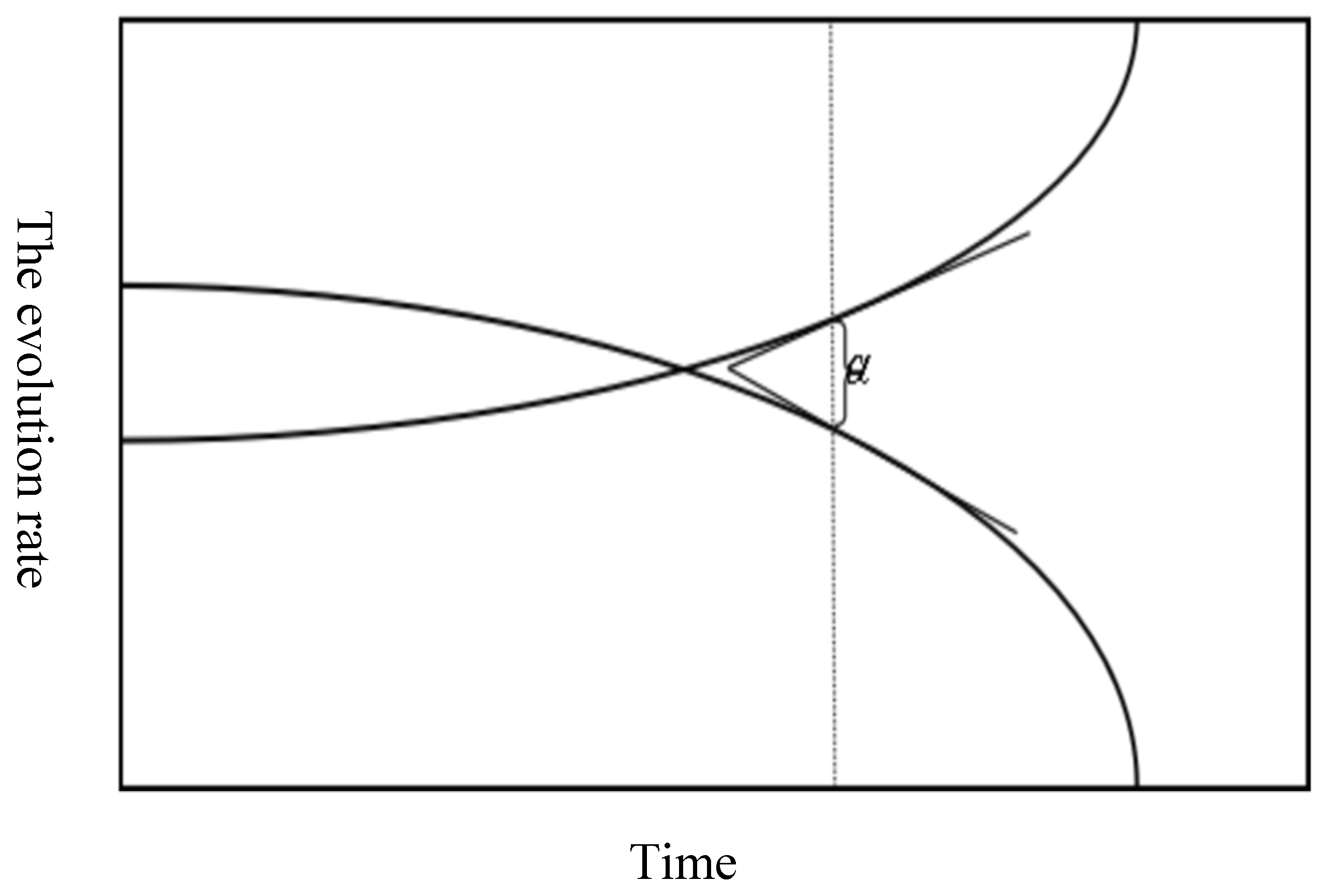
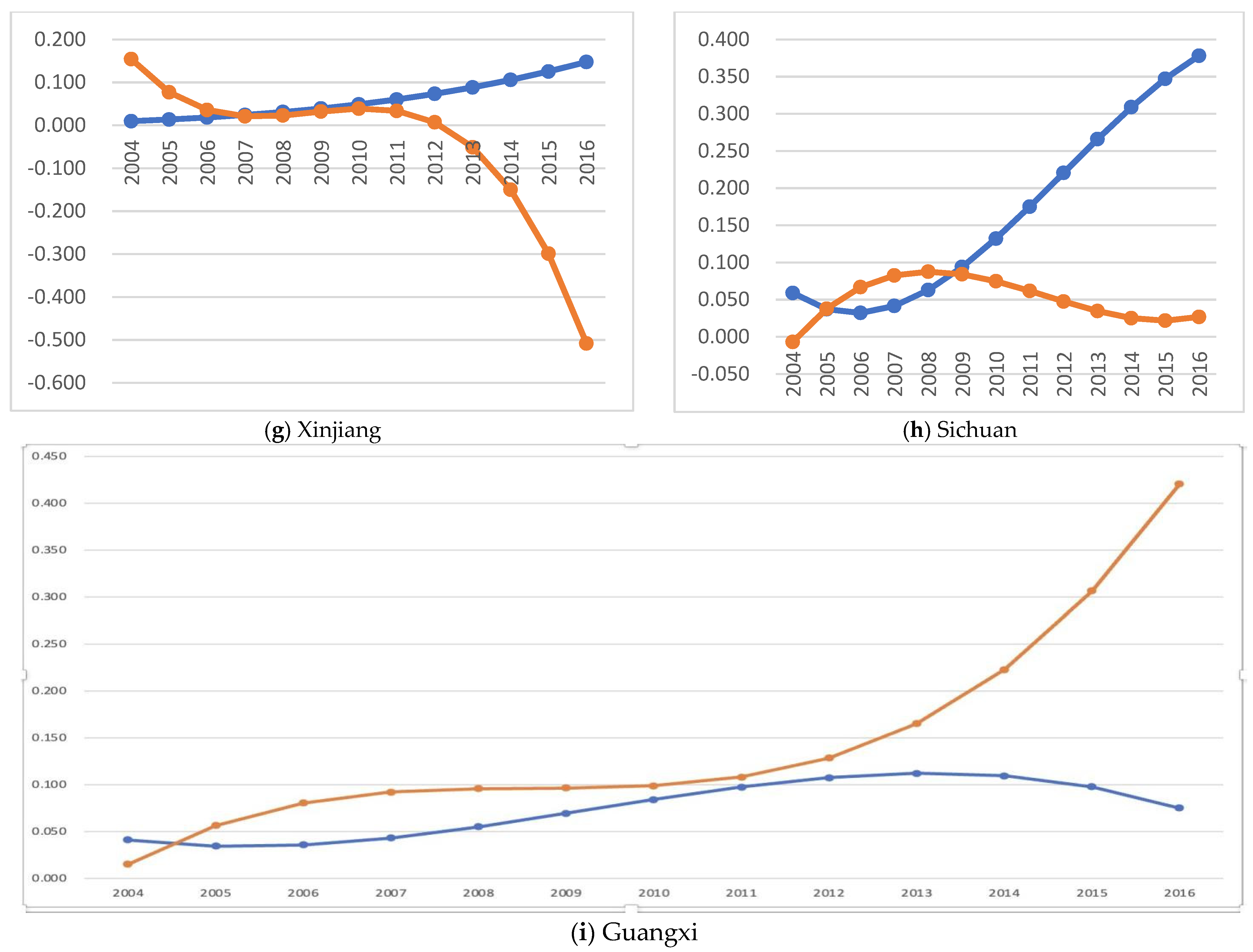
In this paper, we use the scissors difference model to measure the difference in development trends between the sea system and the land system at a given point in time. The larger the scissors difference is, the more significant the difference between the development trends of the two systems (see Figure 2).

The specific calculation process of the scissors difference model is as follows.

Scissors difference model: Suppose the two research systems are x and y. Obtain the coupling equations of the system $F\left(x\right)$ and the system $G\left(y\right)$ by fitting all the comprehensive evaluation values of system $f\left(x\right)$ and system $g\left(y\right)$ in EXCEL. Then, calculate the tangent angle α between $F\left(x\right)$ and $G\left(y\right)$ at a given time. The greater the value of α, the more significant the difference between the x system and y system will be. The specific calculation formula is as follows:

$$V_{F\left(x\right)}=F^{\prime }\left(x\right)=d_x/d_t$$

$$V_{G\left(y\right)}=G^{\prime }\left(y\right)=d_y/d_t$$

$$\alpha =arccos\frac{1+V_{F\left(x\right)}\ast V_{G\left(y\right)}}{\sqrt{\left(1+V_{F\left(x\right)}^2\right)\left(1+V_{G\left(y\right)}^2\right))}}(0\ll \alpha \ll \pi )$$

where the range of t is 1 to 13, corresponding to the years 2004–2016.

2.3.6. Environment Kuznets Curve

Since the 1990s, many research methods have been developed to study the relationship between environmental pollution and economic growth, the most representative of which is the environmental Kuznets curve (EKC), a hypothesis that was proposed by Genegrossman and Kruemeger in 1995. Its core view is that when a country’s economic development level is low, the degree of environmental pollution is low. However, as the economy continues to develop and the per capita income rises, the degree of environmental pollution also continues to increase. However, when the economy grows to a certain level (i.e., after reaching a critical point or an inflection point), environmental pollution will start to decrease. With the continuous development of the economy, ecological quality is improved. The process of ecological decay changes throughout economic growth and exhibits an inverted U-shaped curve, which is called the EKC (Grossman et al., 1994 [46]). The EKC has been observed in some developed countries. Still, some scholars have pointed out that depending on time and regional factors, it does not necessarily have an inverted U-shaped curve but may also have a U-shaped, N-shaped, or cubic curve (Yang et al., 2017 [47]; Ran et al., 2018 [48]).

In domestic and foreign literature, the environmental Kuznets curve is widely used to study the relationship between environmental pollution and economic growth. Yang et al. (2021) conducted a quantitative linear regression analysis of economic growth and environmental pollution in the region based on the Kuznets curve, and they verified the particularity of the Kuznets curve [49]. Li et al. (2021) studied the relationship between environment and economy in 89 Belt and Road countries from 1995 to 2017 and tested the environmental Kuznets curve. The research shows an inverse U-shaped relationship between environmental degradation and economic growth [50]. Cui et al. (2019) summarized the inverted U-shaped environmental Kuznets curve of dynamic evolution from the perspective of an economic development level and development structure based on the traditional Kuznets curve [51].

In recent years, the application scope of the environmental Kuznets curve has been expanding, and more and more scholars have applied it to study the relationship between tourism and ecology. Sun et al. (2021) discussed the relationship between tourism and ecological innovation from 1995 to 2018 under the framework of the environmental Kuznets curve (EKC) [19]. Similarly, Tian et al. (2020) studied the relationship between tourism and environment by using the environmental Kuznets curve, and the research results show that tourism development is the driving force to reduce carbon dioxide emissions [52].

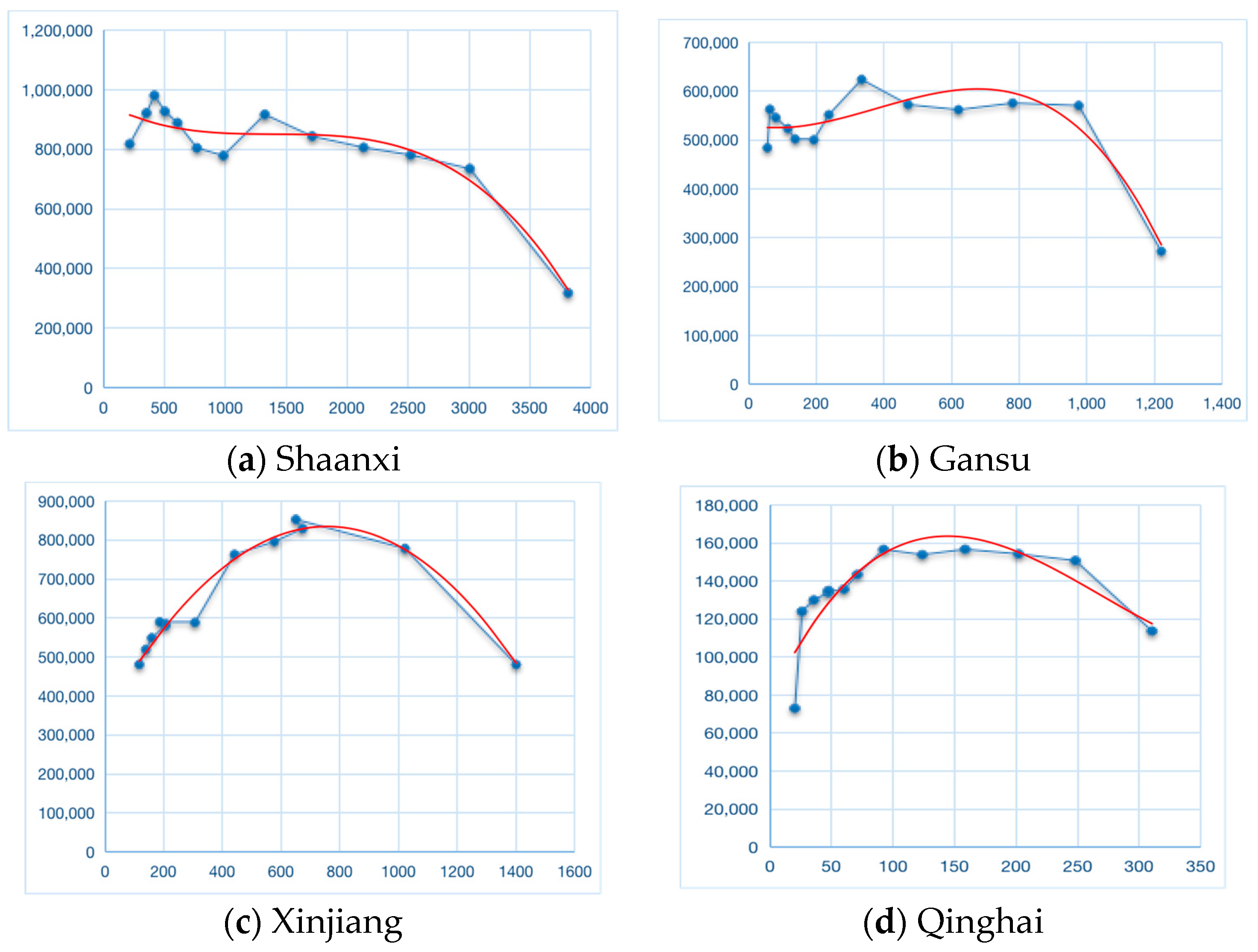
The tourism industry, as a significant pillar of the national economy, has caused severe environmental degradation. In this paper, we construct an EKC model between total tourism revenue, which is used as an evaluation index of the economic level of tourism, and the ecological environment, which is measured by sulfur dioxide emissions, total wastewater discharge, and industrial solid waste generation indicators, to explore the interactive relationship between tourism development and the ecological environment in nine Chinese provinces.

We used SPSS mathematical statistics software to fit the model curve, compare the degree of fit, and determine the EKC of the tourism economic level and the ecological environment level. The basic model is as follows:

$$m_t=\alpha +{\beta }_1\times TGD{P}_t+{\beta }_2\times TGD{P}_t^2+{\beta }_3\times TGD{P}_t^3$$

(17)

where $m_t$ represents the environmental pollution suffered at time $t$; the indicator variables are sulfur dioxide emissions, total wastewater emissions, and industrial solid waste generation; $TGD{P}_t$ represents the total tourism revenue at time $t$; ${\beta }_1$, ${\beta }_2$, and ${\beta }_3$ are parameters to be estimated; and $\alpha$ is a constant term.

Depending on the value of ${\beta }_1$, the shape of the EKC can be classified into the following types, as shown in

Table 3. Different shapes of EKC curve shape.

The Value of ${\mathit{\beta }}_1$$,{\mathit{\beta }}_2$$,{\mathit{\beta }}_3$	EKC Shape	Describe
${\beta }_1>0,{\beta }_2={\beta }_3=0$		There is a monotonic, linear relationship between the environment and income, where the environment deteriorates as income increases.
${\beta }_1<0,{\beta }_2={\beta }_3=0$		There is a monotonically decreasing linear relationship between the environment and income where the environment improves as income increases.
${\beta }_1>0,{\beta }_2<0,{\beta }_3=0$	Inverted “U” shape	That is representative of the EKC, where the inflection point is at the highest point of the curve.
${\beta }_1<0,{\beta }_2>0,{\beta }_3=0$	Positive “U” shape	At the lower income level, the environment improves as income increases, but at the higher income level, the environment deteriorates as income increases.
${\beta }_1>0,{\beta }_2<0,{\beta }_3>0$	Positive “N” shape	As income levels increase, the environment first deteriorates, then improves, and finally deteriorates.
	Increase	There is a monotone, linear relationship between the environment and income, where the environment deteriorates as income increases.
${\beta }_1<0,{\beta }_2>0,{\beta }_3<0$	Inverted “N” shape	As income levels increase, the environment first improves, then deteriorates, and finally improves.
	Decrease	There is a monotonically decreasing, linear relationship between the environment and income, where the environment improves as income increases.

.

3. Results and Interpretation

3.1. The Comprehensive Evaluation Value of the Tourism Subsystem, Transportation Subsystem, and Ecological Environment Subsystem

In the evaluation index system, the tourism subsystem comprehensive evaluation values f_it(x), transportation subsystem comprehensive evaluation values $g_{it}(y)$, and ecological environment subsystem comprehensive evaluation values $k_{it}(z)$ of the nine Chinese provinces from 2004 to 2016 are calculated by Formulas (9)–(11) and are shown in

Table 4. Comprehensive evaluation values of the tourism subsystem, transportation subsystem, and ecological environment subsystem of nine Chinese provinces from 2004 to 2016.

Year	Shaanxi			Gansu			Qinghai			Ningxia			Xinjiang
	${\mathit{f}}_{\mathbf{1}\mathit{t}}(\mathit{x})$	${\mathit{g}}_{\mathbf{1}\mathit{t}}(\mathit{y})$	${\mathit{k}}_{\mathbf{1}\mathit{t}}(\mathit{z})$	${\mathit{f}}_{\mathbf{2}\mathit{t}}(\mathit{x})$	${\mathit{g}}_{\mathbf{2}\mathit{t}}(\mathit{y})$	${\mathit{k}}_{\mathbf{2}\mathit{t}}(\mathit{z})$	${\mathit{f}}_{\mathbf{3}\mathit{t}}(\mathit{x})$	${\mathit{g}}_{\mathbf{3}\mathit{t}}(\mathit{y})$	${\mathit{k}}_{\mathbf{3}\mathit{t}}(\mathit{z})$	${\mathit{f}}_{\mathbf{4}\mathit{t}}(\mathit{x})$	${\mathit{g}}_{\mathbf{4}\mathit{t}}(\mathit{y})$	${\mathit{k}}_{\mathbf{4}\mathit{t}}(\mathit{z})$	${\mathit{f}}_{\mathbf{5}\mathit{t}}(\mathit{x})$	${\mathit{g}}_{\mathbf{5}\mathit{t}}(\mathit{y})$	${\mathit{k}}_{\mathbf{5}\mathit{t}}(\mathit{z})$
2004	0.000	0.015	0.166	0.149	0.062	0.373	0.052	0.028	0.582	0.004	0.052	0.570	0.114	0.009	0.336
2005	0.050	0.062	0.199	0.197	0.077	0.300	0.058	0.058	0.344	0.064	0.085	0.346	0.116	0.050	0.330
2006	0.098	0.152	0.266	0.223	0.126	0.408	0.143	0.156	0.398	0.099	0.125	0.471	0.153	0.150	0.357
2007	0.135	0.220	0.361	0.284	0.167	0.379	0.220	0.198	0.354	0.136	0.167	0.336	0.274	0.222	0.386
2008	0.198	0.304	0.427	0.132	0.304	0.426	0.167	0.285	0.332	0.170	0.306	0.379	0.166	0.259	0.403
2009	0.259	0.348	0.585	0.184	0.361	0.510	0.253	0.335	0.388	0.233	0.412	0.440	0.099	0.287	0.581
2010	0.367	0.502	0.680	0.262	0.425	0.489	0.332	0.409	0.347	0.295	0.553	0.478	0.255	0.320	0.525
2011	0.474	0.599	0.682	0.331	0.519	0.384	0.391	0.525	0.395	0.364	0.698	0.299	0.369	0.460	0.554
2012	0.602	0.659	0.717	0.428	0.615	0.519	0.457	0.589	0.404	0.494	0.824	0.329	0.499	0.619	0.488
2013	0.685	0.672	0.771	0.507	0.613	0.583	0.496	0.520	0.372	0.558	0.735	0.401	0.517	0.776	0.544
2014	0.699	0.818	0.775	0.530	0.730	0.603	0.630	0.567	0.457	0.592	0.806	0.435	0.480	0.844	0.628
2015	0.821	0.814	0.764	0.651	0.806	0.505	0.818	0.756	0.421	0.634	0.828	0.503	0.659	0.860	0.599
2016	0.968	0.843	0.800	0.797	0.906	0.715	0.999	0.822	0.627	0.806	0.804	0.696	0.864	0.832	0.734
Average	0.412	0.462	0.553	0.360	0.439	0.476	0.386	0.404	0.417	0.342	0.492	0.437	0.351	0.438	0.497
Year	Chongqing			Sichuan			Yunnan			Guangxi
	${\mathit{f}}_{\mathbf{6}\mathit{t}}(\mathit{x})$	${\mathit{g}}_{\mathbf{6}\mathit{t}}(\mathit{y})$	${\mathit{k}}_{\mathbf{6}\mathit{t}}(\mathit{z})$	${\mathit{f}}_{\mathbf{7}\mathit{t}}(\mathit{x})$	${\mathit{g}}_{\mathbf{7}\mathit{t}}(\mathit{y})$	${\mathit{k}}_{\mathbf{7}\mathit{t}}(\mathit{z})$	${\mathit{f}}_{\mathbf{8}\mathit{t}}(\mathit{x})$	${\mathit{g}}_{\mathbf{8}\mathit{t}}(\mathit{y})$	${\mathit{k}}_{\mathbf{8}\mathit{t}}(\mathit{z})$	${\mathit{f}}_{\mathbf{9}\mathit{t}}(\mathit{x})$	${\mathit{g}}_{\mathbf{9}\mathit{t}}(\mathit{y})$	${\mathit{k}}_{\mathbf{8}\mathit{t}}(\mathit{z})$
2004	0.002	0.032	0.231	0.021	0.027	0.300	0.002	0.048	0.432	0.000	0.019	0.231
2005	0.081	0.086	0.279	0.058	0.061	0.303	0.066	0.078	0.463	0.073	0.066	0.194
2006	0.102	0.141	0.296	0.129	0.135	0.326	0.098	0.167	0.374	0.101	0.149	0.249
2007	0.141	0.254	0.493	0.170	0.182	0.354	0.124	0.240	0.430	0.123	0.216	0.235
2008	0.204	0.355	0.510	0.128	0.254	0.409	0.144	0.196	0.451	0.154	0.265	0.234
2009	0.274	0.377	0.600	0.196	0.312	0.512	0.205	0.272	0.642	0.205	0.360	0.490
2010	0.380	0.462	0.646	0.289	0.420	0.515	0.293	0.352	0.730	0.305	0.424	0.487
2011	0.476	0.544	0.637	0.372	0.568	0.601	0.377	0.458	0.544	0.401	0.498	0.697
2012	0.627	0.627	0.653	0.578	0.618	0.573	0.520	0.569	0.613	0.541	0.585	0.681
2013	0.656	0.614	0.723	0.626	0.561	0.630	0.639	0.587	0.648	0.619	0.466	0.762
2014	0.786	0.701	0.669	0.702	0.666	0.655	0.695	0.699	0.697	0.702	0.577	0.793
2015	0.866	0.739	0.718	0.817	0.711	0.660	0.808	0.787	0.686	0.805	0.677	0.826
2016	0.987	0.789	0.712	0.950	0.774	0.736	1.045	0.909	0.786	0.949	0.738	0.844
Average	0.429	0.440	0.551	0.387	0.407	0.506	0.386	0.412	0.577	0.383	0.388	0.517

.

It can be seen in Table 4 that from 2004 to 2016, the development trends of the tourism and transportation systems in the Silk Road Economic Belt of the nine provinces were basically the same, and their comprehensive evaluation values significantly improved. In Gansu, Ningxia, and Xinjiang, the growth in comprehensive evaluation values for the tourism system was greater than that of the transportation system. Among the remaining six provinces, Yunnan experienced the most significant growth in its tourism system, while Gansu saw the most negligible change. Yunnan was also the province that experienced the most significant change in its transportation system, while Guangxi saw the least growth. Between 2004 and 2012, the comprehensive evaluation values of the transportation system in Gansu, Ningxia, and Xinjiang were higher than that of the tourism system compared to the other six provinces. However, this trend was reversed when considering the remaining provinces between 2013 and 2016, noting that 2013 was the first year of the Belt and Road strategy. Thus, the proposal of the One Belt, One Road strategy is of great strategic significance for promoting tourism in the provinces along the route in China. Since before 2007, Gansu, Ningxia, and Xinjiang have possessed an inherent advantage in tourism but a geographical location disadvantage in transportation; as a result, their tourism industries are relatively more developed than their transportation industries. Following the Qinghai–Tibet railway, which opened in 2006, the transportation industry began to grow rapidly, eventually to a more significant extent than the tourism industry. Thus, in China, national policy support plays a crucial role in promoting the development of transportation infrastructure.

The evolution trends of the comprehensive evaluation values for the ecological environment are inconsistent. Ecological environment evaluation values for Shaanxi, Sichuan, and Yunnan steadily increased, but they fluctuated on a generally upward trend for the remaining six provinces. The fluctuations were the most pronounced in Ningxia, which dropped from 0.570 in 2004 to a low of 0.299 in 2011, before rising to 0.696 by 2016. Regions with highly developed tourism and transportation industries have begun to recognize the importance of sustainable development. In areas where the tourism and transportation industries are relatively less advanced, the coordinated development of tourism, transportation, and the ecological environment is still in the exploratory stage.

3.2. Coupling Coordination Degree of the TTE System

The comprehensive evaluation values of the TTE system were substituted into the coupling coordination degree evaluation model to obtain the coupling coordination degree values of the TTE system of each province from 2004 to 2016, as shown in

Table 5. Coupling coordination degree of the TTE system of each province from 2004 to 2016.

Year	Shaanxi	Gansu	Qinghai	Ningxia	Xinjiang	Chongqing	Sichuan	Yunnan	Guangxi
2004	0.01	0.39	0.31	0.22	0.27	0.15	0.24	0.19	0.01
2005	0.29	0.41	0.32	0.35	0.35	0.35	0.32	0.36	0.31
2006	0.40	0.48	0.45	0.42	0.45	0.40	0.42	0.42	0.39
2007	0.47	0.51	0.50	0.44	0.54	0.51	0.47	0.48	0.43
2008	0.54	0.51	0.50	0.52	0.51	0.58	0.49	0.48	0.46
2009	0.61	0.57	0.57	0.59	0.50	0.63	0.56	0.57	0.58
2010	0.71	0.62	0.60	0.65	0.59	0.70	0.63	0.64	0.63
2011	0.76	0.64	0.66	0.65	0.67	0.74	0.71	0.67	0.72
2012	0.81	0.72	0.69	0.72	0.73	0.80	0.77	0.75	0.77
2013	0.84	0.75	0.68	0.74	0.78	0.81	0.78	0.78	0.78
2014	0.87	0.78	0.74	0.77	0.80	0.85	0.82	0.83	0.83
2015	0.89	0.80	0.80	0.80	0.84	0.88	0.85	0.86	0.88
2016	0.93	0.90	0.90	0.88	0.90	0.91	0.90	0.94	0.92

. The system coupling coordination degree of the nine provinces has generally developed toward good coordination, and all have experienced the three stages of uncoordinated development, transformational development, and coordinated development. From 2004 to 2005, the nine provinces were in uncoordinated development. While most provinces were in a state of mildly uncoordinated development by 2005, Shaanxi and Guangxi were in extremely uncoordinated development in 2004, and Chongqing and Yunnan were in severely uncoordinated development at the same time. From 2006 to 2009, the nine provinces transitioned from uncoordinated states to coordinated development states. Shaanxi and Chongqing were the first to reach coordinated development, whereas the speed of transformation for Sichuan, Yunnan, and Guangxi was slow. From 2010 to 2016, the nine provinces were all in a state of coordinated development, although Gansu, Ningxia, and Qinghai were slower to transition. As of 2016, all provinces were in a state of well-coordinated development.

Capital and technology accumulation in the early development of the tourism and transportation industries, as well as the popularization of environmental protection concepts, have restored the ecological environment and eased environmental pressure to a certain extent.

However, it is worth noting that except for Gansu, Qinghai, and Xinjiang, before 2013, the remaining six provinces lagged in tourism development, which was slower to grow than the construction of transportation facilities. After implementing the Belt and Road strategy, the rapid growth of the tourism industry narrowed the development gap between the tourism and transportation industries. In fact, since 2014, the comprehensive development level of the tourism industry has surpassed that of the transportation industry. Since 2015, the development of an extensive tourism economy and the construction of transportation facilities have caused considerable damage to the ecological environment. Coupled with the overexploitation of tourism resources and the inadequate control of environmental pollution, the ecological environment’s restrictive effect on the tourism and transportation industries has gradually emerged.

3.3. The Mean Square Error Index of the Coupling Coordination Degree

The mean square error index and the contribution rate of the overall difference $S$, interregional difference $S_1$, and interprovincial difference $S_2$ of the coupling coordination degree from 2004 to 2016 are calculated using Formulas (15) and (16) and are shown in

Table 6. The mean square error index of each province from 2004 to 2016.

Year	$\mathit{S}$	${\mathit{S}}_{\mathbf{1}}$	Contribution Rate	${\mathit{S}}_{\mathbf{2}}$	Contribution Rate	${\mathit{S}}_{\mathbf{2}}$ North	Contribution Rate	${\mathit{S}}_{\mathbf{2}}$ South	Contribution Rate
2004	0.0690	0.0020	2.95%	0.0670	97.05%	0.0496	74.05%	0.0174	25.95%
2005	0.0049	0.0000	0.30%	0.0049	99.70%	0.0041	82.53%	0.0009	17.47%
2006	0.0034	0.0002	6.12%	0.0032	93.88%	0.0025	76.29%	0.0008	23.71%
2007	0.0049	0.0001	1.90%	0.0048	98.10%	0.0030	63.96%	0.0017	36.04%
2008	0.0046	0.0001	1.28%	0.0045	98.72%	0.0008	16.77%	0.0038	83.23%
2009	0.0052	0.0001	1.08%	0.0052	98.92%	0.0038	72.84%	0.0014	27.16%
2010	0.0066	0.0001	0.99%	0.0066	99.01%	0.0051	78.18%	0.0014	21.82%
2011	0.0082	0.0003	3.38%	0.0079	96.62%	0.0060	76.43%	0.0019	23.57%
2012	0.0072	0.0004	4.99%	0.0069	95.01%	0.0055	79.57%	0.0014	20.43%
2013	0.0096	0.0002	2.41%	0.0093	97.59%	0.0084	89.94%	0.0009	10.06%
2014	0.0076	0.0004	4.64%	0.0072	95.36%	0.0063	86.79%	0.0010	13.21%
2015	0.0061	0.0004	6.64%	0.0057	93.36%	0.0046	80.75%	0.0011	19.25%
2016	0.0017	0.0001	4.28%	0.0016	95.72%	0.0011	65.63%	0.0006	34.37%

. Figure 3 shows that the total mean square error index displayed a downward trend from 2004 to 2016, indicating that the difference in the coupling coordination degree of the tourism system, transportation system, and eco-environmental system gradually decreased. The interprovincial differences were far greater than the regional differences. Among the overall differences, the contribution rate of the interprovincial differences was significant. Among the interprovincial differences, the contribution rate of the northern provinces was much higher than that of the southern provinces (i.e., there was a “strong south and weak north”).

3.4. The Scissors Difference between the Tourism System and Transportation System

According to the calculation formula of the scissors difference model, the scissors difference between the tourism system and the transportation system (i.e., the difference in the evolution rate of the two systems) of the nine provinces can be obtained from the scissors difference model, as shown in Figure 4. Between 2004 and 2016, the differences in the evolution rate between the tourism and transportation systems in Shaanxi, Yunnan, Qinghai, and Chongqing were relatively small, with the most miniature scissors difference being in Chongqing at 1.1°. Before 2009, the evolution rate of the transportation system in Shaanxi, Yunnan, Chongqing, and Qinghai was higher than that of the tourism system. However, after 2009, this trend reverses. The evolution rate of the tourism system and transportation system in Gansu, Xinjiang, Ningxia, Guangxi, and Sichuan was relatively low before 2010. The scissors difference between the two systems increased after 2010. As of 2016, Xinjiang had the largest scissors difference at 35.3°, which was followed by Gansu Province with a scissors difference of 30.7°.

The evolution rate of the tourism and transportation systems in nine Chinese provinces from 2004 to 2016 is shown in Figure 5. There is very close interdependence between tourism and transportation systems. A transportation system is a prerequisite and an essential factor for developing the tourism system. The continuous improvement of the transportation system has improved the timeliness and convenience of tourism activities and promotes the development of the tourism system. Before 2009, the transportation system in the studied nine provinces developed faster than the tourism system, but this growth supported the development of regional tourism in later years. In fact, since 2009, tourism has been overgrowing, whereas the development of the transportation system has dropped significantly, which is a trend that will limit the future development of the tourism industry.

3.5. The EKC of the Tourism System and Ecological Environment System

From the basic EKC model, the EKC fitting formula for the tourism economy and ecological environment in the nine provinces can be calculated (see Appendix D for details).

3.5.1. EKC Model of Total Tourism Revenue and Sulfur Dioxide Emissions

We can draw the following conclusions from the results of fitting the EKC with total tourism revenue and sulfur dioxide emissions (As shown in Figure 6). Between 2004 and 2016, the EKCs of Shaanxi, Chongqing, and Sichuan had no inflection points and showed a decreasing trend. Sulfur dioxide emissions declined as total tourism revenue increased. The EKCs of Gansu, Ningxia, and Guangxi were inverted N-shaped with two inflection points. For Gansu, the first turning point appeared between 2006 and 2007, and the second appeared between 2013 and 2014. Before 2007, the environment continuously deteriorated as the tourism economy developed. From 2007 to 2013, environmental quality improved as the tourism economy grew. However, from 2013 to 2016, ecological quality began to deteriorate again with the continuous development of the tourism economy. Xinjiang’s EKC curve was U-shaped with only one turning point that appeared between 2014 and 2015. Generally, before 2014, ecological quality improved as the tourism economy grew, but after 2015, this trend reversed. The EKC curves in Qinghai and Yunnan were positive N-shaped with two inflection points. In Qinghai, the first turning point appeared between 2012 and 2013 and the second turning point appeared after 2016; i.e., the environmental quality first improved and then deteriorated as the tourism economy developed.

3.5.2. EKC Model of Total Tourism Revenue and Total Wastewater Discharge

We can draw the following conclusions from the results of fitting the EKC with total tourism revenue and total wastewater discharge. From 2004 to 2016, the EKCs of Shaanxi and Yunnan exhibited an increasing trend without an inflection point. Sichuan showed an inverted N-shape, and the only inflection point with practical significance was the second turning point that appeared after 2016. The remaining five provinces had EKCs with positive N-shapes and two turning points. The interaction analysis between environmental quality and the tourism economy is the same as in Section 3.5.1.

3.5.3. EKC Model of Total Tourism Revenue and Industrial Solid Waste Generation

The EKC model results of total tourism revenue and industrial solid waste generation are shown in

Table 7. EKC curves for nine provinces from 2004 to 2016.

Ecological Environment Indicators	Shaanxi	Gansu	Qinghai	Ningxia	Xinjiang	Chongqing	Sichuan	Yunnan	Guangxi
Sulfur dioxide emissions	Decrease progressively	Inverted N-type	Positive N-type	Inverted N-type	Inverted U-type	Decrease progressively	Decrease progressively	Positive N-type	Inverted N-type
Total waste water emissions	Increase progressively	Positive N-type	Positive N-type	Positive N-type	Positive N-type	Positive N-type	Inverted N-type	Increase progressively	Positive N-type
Industrial solid waste production volume	Positive N-type	Positive N-type	Increase progressively	Positive N-type	Positive N-type	Positive N-type	Inverted U-type	Inverted U-type	Positive N-type

. We can draw the following conclusions from the results of fitting the EKC with the total tourism revenue and industrial solid waste generation. The EKC of Ningxia had an increasing trend without an inflection point. Sichuan and Yunnan had an inverted U-shape with only one inflection point. The remaining six provinces all had a positive N-shape with two inflection points. The interaction analysis between environmental quality and the tourism economy is also in Section 3.5.1. The interactive relationship between tourism, economic development, and environmental quality is in constant flux. With the development of the tourism economy, improvement of environmental protection capabilities, and change in consumer travel demand, environmental quality will show a good development trend for a period of time. However, large-scale and extensive development of the tourism economy will overcrowd tourism destinations, destroy the ecological environment, and worsen pollution. Without safeguards, the environmental quality will begin to deteriorate, which will restrict high-quality development of the tourism economy.

4. Conclusions and Policy Recommendations

4.1. Conclusions

In this paper, we constructed an index evaluation system of the coupling and coordination relationship of the TTE system. Then, we empirically analyzed the evolution of the coupling coordination degree and comprehensive evaluation values of nine Chinese provinces along the Silk Road Economic Belt from 2004 to 2016 through coupling coordination, mean square error index, scissors difference, Kuznets curve, and other models. We draw the following conclusions:

(1)

Judging from their comprehensive evaluation scores, while the state of the ecological environment system can exhibit an upward or downward trend depending on the stage of development, the tourism and transportation systems are on an overall upward trend, where the transportation and economic systems are evolving toward a stage of common development. The excessive development and traffic planning of tourism resources caused a series of ecological environment problems, affected the sustainable development of the transportation system actively adapting to the new situation request, insisted on high-quality development, promoting the comprehensive transportation, intelligent transportation, safe transportation, and green transportation construction, and walked the road of the new age transportation development.

(2)

The coupling and coordination relationship of the tourism–transportation–ecological environment in the nine provinces along the Silk Road Economic Belt in China is generally developing in a well-coordinated direction. With the implementation of the Belt and Road Initiative, provinces are experiencing a transformation from uncoordinated development to coordinated development. Although the conversion speed is not consistent, the strengthening of coordination is conducive to creating a harmonious and inclusive cultural environment. The surrounding cities promote all-round cooperation in culture, art, tourism, academia, medical treatment, and science and technology to strengthen the coordination of the tourism system in the three coupling systems and at the same time drive the coordination of the ecological environment, protect the eastern, central, and western ecological regions to a certain extent, and promote the sustainable development of the environment.

(3)

The total difference in the coupling coordination degree of the tourism system, transportation system, and ecological environment system of each province is narrowing. The interprovincial difference is more significant than the interregional difference; however, within regions, the difference between northern provinces is more significant than between southern provinces, exhibiting a trend of “strong in the south and weak in the north”. The degree of coupling and coordination among provinces needs to be strengthened. Under the Silk Road spirit of peace, cooperation, openness, and win–win, provinces should be endowed with the connotation of equality, inclusiveness, and mutual learning to achieve a coordinated development and harmonious coexistence.

(4)

The scissors difference in the evolution rate between the tourism and transportation systems first shrinks and then expands, showing a strong dependence between them. The development of the transportation industry precedes the development of tourism, promotes the optimal allocation of regional factor resources, and provides support for the development of the tourism economy. The sound development of the tourism economic system is conducive to creating a peaceful and stable surrounding environment, puts forward better requirements for the transportation industry, and further drives the development of transportation. The collaborative development of the two means that China’s tourism industry will implement the new development concept of innovation, coordination, green, open and sharing, and centering on and serving the Belt and Road strategy, which is of constructive significance to optimize the internal and external environment of China’s development.

(5)

There is a strong correlation between tourism, economic growth, and environmental quality, but it generally does not conform to the inverted U-shaped EKC. There are positive N, inverted N, and increasing, decreasing, and inverted U-shapes and other curves. Environmental quality may be improved or deteriorate depending on the state of tourism economic development, so the relationship between the tourism economy and environmental quality is constantly alternating. On the one hand, it is necessary to follow the precautionary principle. Ecologically sustainable development is the ecological foundation of sustainable development. On the other hand, the environment should be kept healthy, diverse, and productive for the benefit of the next generation.

4.2. Policy Recommendations

The coupling and coordination levels of the TTE system in each province indicate a state of interregional imbalance, and the degree of coordination needs to be improved. Therefore, we propose the following policy recommendations:

(1)

Adjust the structure of the tourism industry, vigorously develop ecotourism and low-carbon tourism, limit expansion, focus on quality improvement, strengthen policy coordination among tourism-related departments, and improve tourism competition mechanisms. Furthermore, increase tourism talent training, promote cross-border scientific research and project cooperation, and improve the cultural soft power of the Silk Road. Seize the opportunity of developing the Belt and Road strategy, change the existing tourism development mode, avoid “high consumption and high pollution”, and realize the sustainable development of tourism.

(2)

Improve the tourism transportation infrastructure system by increasing connectedness, comfort, and speed. Construct more highways, reduce geographical restrictions and administrative barriers to highway construction, and improve the accessibility of tourist attractions in remote provinces. For example, the Yaxi Expressway dramatically shortens the time for central and eastern Sichuan to enter western Sichuan and enhances the accessibility of scenic spots along the line. Create a high-quality rapid transportation network, ensure efficient service on the basis of common arteries of communication and wide coverage, and speed up the formation of the three-dimensional interconnection of the comprehensive traffic network pattern; construction can pass adjacent provinces, in an inline grid around the railway, in the province to achieve the Silk Road Economic Belt in more than nine provinces in the development of scenic spots together, and release the provinces along with the development potential. We should achieve common growth and prosperity through mutual benefit and win–win cooperation and foster a peaceful, stable, and harmonious neighborhood. For example, relying on its geographical advantage, Xinjiang has issued a series of action plans, proposing to build the Silk Road Economic Belt and accelerate the construction of five centers. Shanxi also mentioned that it should be built into a new starting point and bridgehead of the northwest region’s foreign economy. Gansu will build the golden section of the Silk Road Economic Belt, build the Lanzhou New Area logistics park, and open the Lanzhou international logistics special line; Qinghai grasped the opportunity of the construction of the Silk Road Economic Belt, expanded the breadth and depth of opening to the outside world, built a strategic channel connecting domestic and foreign countries, and made the construction of the Silk Road Economic Belt become a new economic growth point of Qinghai’s development. Ningxia is following the banner of the Belt and Road strategy to build a strategic fulcrum connecting China and the outside world.

(3)

The tourism ecological environment along the Silk Road Economic Belt has been damaged, and the cooperation of environmental protection should be emphasized in the development of the tourism economy and the construction of transportation infrastructure. By strengthening the construction of software infrastructure, natural conditions can be improved, the accountability system for environmental problems can be improved, the awareness of environmental protection of tourism subjects can be enhanced, and the sustainable growth can be satisfied to a greater extent. At the same time, it will increase the fiscal revenue of provinces along the Belt and Road, attract investment, prepare the necessary material and technological conditions for further development, and promote the sustainable development of the population, resources, and environment.

5. Research Implications

In this paper, provinces along the Belt and Road in China were selected as the research object to systematically analyze the coupling and coordination of the tourism system, transportation system, and ecological environment system. However, there are still some deficiencies in this study, which need to be further improved and supplemented in future research.

(1)

In the synergy of the TTE system, there is an interactive relationship between tourism, the transportation system, and the ecological environment system. Although tourism is in the core position, due to the ‘short-board effect’, it is not enough to emphasize the rapid development of tourism, the improvement of transportation facilities, and the protection of the ecological environment. Therefore, in future development, all provinces and cities should pay full attention to the regional short board, optimize policy guidance, reasonably formulate industrial development policies in line with the region, improve the shortboard, build a tourism development coordination mechanism from the technical level, and optimize and accelerate the coordinated development of the TTE system.

(2)

China’s inherent administrative barriers have always been a critical obstacle factor affecting the development of industrial integration between provinces. Therefore, in the future process of regional coordinated development, we should break administrative barriers, strengthen exchanges and cooperation between provinces (cities), promote the integrated construction of the tourism economy, transportation services, and ecological environment, and realize the overall coordinated and rapid growth of the regional economy. At the same time, we should pay more attention to the spatial relevance of industries and reduce the restrictions of other industries on the development of the tourism industry.

(3)

So far, research on the coupling coordination degree of the TTE system is still in the initial exploration stage. The details are presented as follows. (1) In the study area, this paper takes nine provinces along the Belt and Road in China as the research area, and the research scope is single and limited. In future, comparing and analyzing regional scales, such as the economic belt and urban agglomeration, should be considered. (2) In the research methods, on the one hand, the availability of the data indicators adopted in the index system in this paper are measurable and supported by data. However, some qualitative indicators, such as the tourism culture of the tourism system, intelligentization of the transportation system, and the sustainable development ability of the ecosystem can be further supplemented and improved in the future. On the other hand, in this paper, the cosine law method and entropy weight method were used to determine the weight of each evaluation index, both of which are objective evaluation methods. There is no subjective evaluation method in this paper, and future research can adopt a combination of subjective and objective methods.

References

1. Jaarsma, C.F.; Beunen, R.; Kooij, H.J. Traffic management at leisure destinations in the countryside: An integrated approach for transportation and tourism planning. Ann. Fam. Med. 2008, 241, 269–270. [Google Scholar]
2. Houts, D.V. Airtransport and international tourism: An examination of the distribution of the benefits between developed and developing countries. Tour. Rev. 2013, 39, 16–18. [Google Scholar] [CrossRef]
3. Carolina, S.J. Transport and tourism in brazil: An ongoing movement. Mobil. Hist. 2015, 6, 165–171. [Google Scholar]
4. Alkheder, S.A. Transportation and tourism sustainability in major jordanian tourism cities. Tour. Plan. Dev. 2016, 13, 253–273. [Google Scholar] [CrossRef]
5. Sharkhuu, O.; Yongjian, P.U.; Bayasgalan, T. The Impact of Transport Infrastructure and Pollutant Emissions in Sustainable Tourism for Mongolia. Int. J. Tour. Hotel. Manag. 2020, 8, 12. [Google Scholar]
6. Wang, Y.; Wang, M.; Li, K.; Zhao, J. Analysis of the Relationships between Tourism Efficiency and Transport Accessibility—A Case Study in Hubei Province, China. Sustainability 2021, 13, 8649. [Google Scholar] [CrossRef]
7. Wendt, J.A.; Grama, V.; Ilieş, G.; Mikhaylov, A.S.; Borza, S.G.; Herman, G.V.; Bógdał-Brzezińska, A. Transport Infrastructure and Political Factors as Determinants of Tourism Development in the Cross-Border Region of Bihor and Maramure. A Comparative Analysis. Sustainability 2021, 13, 5385. [Google Scholar] [CrossRef]
8. Papatheodorou, A. A review of research into air transport and tourism. Ann. Tour. Res. 2021, 87, 103151. [Google Scholar] [CrossRef]
9. Hill, W.; Pickering, C.M. Vegetation associated with different walking track types in the Kosciuszko alpine area, Australia. J Environ. Manag. 2006, 78, 24–34. [Google Scholar] [CrossRef]
10. Burgin, S.; Hardiman, N. The direct physical, chemical and biotic impacts on australian coastal waters due to recreational boating. Biodivers. Conserv. 2011, 20, 683–701. [Google Scholar] [CrossRef]
11. Xuan, F.H. The Coupling Development between Tourism Economy and Ecology environment in Harbin City. Adv. Mater. Res. 2013, 726, 4150–4153. [Google Scholar]
12. Huang, C.Q.; Peng, H.J. Evaluation Index System of Tourism Ecology environment Security of Islet in River and it’s Application. Adv. Mater. Res. 2013, 788, 379–382. [Google Scholar]
13. Gon, M.; Osti, L.; Pechlaner, H. Leisure boat tourism: Residents’ attitudes towards nautical tourism development. Tour. Rev. 2016, 71, 180–191. [Google Scholar] [CrossRef]
14. Zhong, L.; Zhang, X.; Deng, J.; Pierskalla, C. Recreation Ecology Research in China’s Protected Areas: Progress and Prospect. Ecosyst. Health Sustain. 2020, 6, 13. [Google Scholar] [CrossRef]
15. Yong, E.L. Understanding the Economic Impacts of Sea-Level Rise on Tourism Prosperity: Conceptualization and Panel Data Evidence. Adv. Clim. Chang. Res. 2021, 12, 240–253. [Google Scholar] [CrossRef]
16. Daigle, P. A summary of the environmental impacts of roads, management responses, and research gaps: A literature review. J. Ecosyst. Manag. 2010, 10, 66–90. [Google Scholar]
17. Zhou, Q.F.; Liu, L. Integrated Transport Development and Ecological Environment Game Identification. Advances in Computer Science, Intelligent System & Environment. DBLP 2011, 106, 165–170. [Google Scholar]
18. Zhou, Q.; Si, M.A.; Luo, Y. Harmonious Relations of Transportation Energy Consumption in Integrated Transport Development. J. Transp. Syst. Eng. Inf. Technol. 2012, 12, 11–16. [Google Scholar] [CrossRef]
19. Sun, Y.; Duru, O.A.; Razzaq, A.; Dinca, M.S. The asymmetric effect eco-innovation and tourism towards carbon neutrality target in Turkey. J. Environ. Manag. 2021, 299, 113653. [Google Scholar] [CrossRef]
20. Ma, T.S.; Fan, Y.J. Study of transportation and strategy of energy and environment in China. J. Traffic Transp. Eng. 2008, 8, 116–120. [Google Scholar]
21. Wang, M.M.; Kong, Y.P.; Chen, B.; Gu, X.F. Concept, Attributes and Classification of Tourism Highway in China. Highway 2019, 3, 176–181. [Google Scholar]
22. Li, S.; Xing, J.; Yang, L.; Zhang, F. Transportation and the Environment in Developing Countries. Annu. Rev. Resour. Econ. 2020, 12, 389–409. [Google Scholar] [CrossRef]
23. Shu, X.; Gao, Y.; Zhang, Y.; Yang, C. Study on the coupling relationship and coordinated development between tourism industry and ecological civilization city. J. Resour. Ecol. 2015, 25, 82–90. [Google Scholar]
24. Fei, J.; Lin, Y.; Jiang, Q.; Jiang, K.; Li, P.; Ye, G. Spatiotemporal coupling coordination measurement on islands’ economy-environment-tourism system. Ocean. Coast. Manag. 2021, 212, 105793. [Google Scholar] [CrossRef]
25. Han, H.; Guo, L.; Zhang, J.; Zhang, K.; Cui, N. Spatiotemporal analysis of the coordination of economic development, resource utilization, and environmental quality in the Beijing-Tianjin-Hebei urban agglomeration. Ecol. Indic. 2021, 127, 107724. [Google Scholar] [CrossRef]
26. Tang, Z. An integrated approach to evaluating the coupling coordinationbetween tourism and the environment. Tour. Manag. 2015, 46, 11–19. [Google Scholar] [CrossRef]
27. Wu, H.; Liu, D. Study on the coupling coordination degree of Transportation and tourism development in China. Econ. Empir. 2019, 17, 143–146. [Google Scholar]
28. Xu, H.Y.; Zheng, H.D.; Wu, L. Analysis on coupling coordination of tourism industry, urbanization, ecology environment—A case study of six provinces along the middle and lower reaches of the Yangtze river. J. Fujian Agric. For. Univ. 2017, 20, 84–92. [Google Scholar]
29. Shannon, C.E. A mathematical theory of communication. Bell Labs Tech. J. 1948, 27, 379–423. [Google Scholar] [CrossRef] [Green Version]
30. Zhang, M.; Ma, J.; Zhao, W.; Wang, X. Groundwater Environmental Quality Evaluation Based on the Entropy Weight Method. In Proceedings of the International Conference on Environmental Technology and Knowledge Transfer, Hefei, China, 15–16 May 2014. [Google Scholar]
31. Wang, C.; Xu, M.; Olsson, G.; Liu, Y. Characterizing of water-energy-emission nexus of coal-fired power industry using entropy weighting method. Resour. Conserv. Recycl. 2020, 161, 104991. [Google Scholar] [CrossRef]
32. Yan, J.H.; Feng, C.H.; Li, L. Sustainability assessment of machining process based on extension theory and entropy weight approach. Int. J. Adv. Manuf. Technol. 2014, 71, 1419–1431. [Google Scholar] [CrossRef]
33. Jesmin, F.K.; Sharif, M.B. Weighted entropy for segmentation evaluation. Opt. Laser Technol. 2014, 57, 236–242. [Google Scholar]
34. Lai, C.; Chen, X.; Wang, Z.; Wu, X. A fuzzy comprehensive evaluation model for flood risk based on the combination weight of game theory. Nat. Hazards 2015, 77, 1243–1259. [Google Scholar] [CrossRef]
35. Zhao, L.M.; Li, L.; Wu, Y.J. Research on the Coupling Coordination of a Sea–Land System Based on an Integrated Approach and New Evaluation Index System: A Case Study in Hainan Province, China. Sustainability 2017, 9, 859. [Google Scholar] [CrossRef] [Green Version]
36. Wang, Q.; Li, S. Shale gas industry sustainability assessment based on WSR methodology and fuzzy matter-element extension model: Thecase study of China. J. Clean. Prod. 2019, 226, 336–348. [Google Scholar] [CrossRef]
37. Zhu, D.; Wang, R.; Duan, J.; Cheng, W. Comprehensive weight method based on game theory for identify criticaltransmission lines in power system. Electr. Power Energy Syst. 2021, 124, 106362. [Google Scholar] [CrossRef]
38. Zuo, Z.; Guo, H.; Cheng, J.; Li, Y. How to achieve new progress in ecological civilization construction? - Based on cloud model and coupling coordination degree model. Ecol. Indic. 2021, 127, 107789. [Google Scholar] [CrossRef]
39. Liu, T.L.; Song, Q.J.; Lu, J.; Qi, Y. An integrated approach to evaluating the coupling coordination degree between low-carbon development and air quality in Chinese cities. Adv. Clim. Chang. Res. 2021, 12, 710–722. [Google Scholar] [CrossRef]
40. Wang, R.; Cheng, J.; Zhu, Y.; Lu, P. Evaluation on the coupling coordination of resources and environment carrying capacity in Chinese mining economic zones. Resour. Policy 2017, 53, 20–25. [Google Scholar] [CrossRef]
41. Zhang, S.L.; Xu, H.Y.; Zou, Q. Spatio-Temporal Differences between Tourism Economy and Traffic System in China Silk Road Economic Belt. J. Zhongzhou Univ. 2018, 35, 30–35. [Google Scholar]
42. Seton, F. Scissor crises, value-prices, and the movement of value-prices under technical change. Struct. Chang. Econ. D 2000, 11, 13–24. [Google Scholar] [CrossRef]
43. Yue, D.; Xu, X.; Li, Z.; Hui, C.; Li, W.; Yang, H.; Ge, J. Spatiotemporal analysis of ecological footprint and biological capacity of Gansu, China 1991–2015: Down from the environmental cliff. Ecol. Econ. 2006, 58, 393–406. [Google Scholar] [CrossRef]
44. Liu, Y.; Yang, L.; Jiang, W. Coupling coordination and spatiotemporal dynamic evolution between social economy and water environmental quality—A case study from Nansi Lake catchment, China. Ecol. Indic. 2020, 119, 106870. [Google Scholar] [CrossRef]
45. Su, S. Study on coupling coordination between Ecological environment and economic Development in Ningxia Hui Autonomous Region. Res. Soil Water Conserv. 2021, 28, 367–374. [Google Scholar]
46. Grossman, G.M.; Krueger, A.B. Economic Growth and the Environment. Q. J. Econ. 1994, 110, 353–377. [Google Scholar] [CrossRef] [Green Version]
47. Yang, X.; Lou, F.; Sun, M.; Wang, R.; Wang, Y. Study of the relationship between greenhouse gas emissions and the economic growth of Russia based on the Environmental Kuznets Curve. Appl. Energy 2017, 193, 162–173. [Google Scholar] [CrossRef]
48. Ran, Z.; Mengzhen, Z.; Junbo, X. Industrial Transfer, Economic Growth and Enrironmental Pollution: An Inspiration from the Environmental Kuznets Curve. Ecol. Econ. 2018, 34, 68–73. [Google Scholar]
49. Yang, H.A.; Ma, J.B. Correlation analysis between regional economic differences and environmental pollution based on Kuznets curve model. Environ. Technol. Innov. 2021, 22, 101444. [Google Scholar] [CrossRef]
50. Li, W.; Qiao, Y.; Li, X.; Wang, Y. Energy consumption, pollution haven hypothesis, and Environmental Kuznets Curve: Examining the environmenteeconomy link in belt and road initiative countries. Energy 2021, 239, 122559. [Google Scholar] [CrossRef]
51. Cui, X.; Han, M.; Fang, Z. Kuznets curve of inverted u-shaped environment with dynamic evolution. China Popul. Resour. Environ. 2019, 29, 74–82. [Google Scholar]
52. Tian, X.L.; Bélaïd, F.; Ahmad, N. Exploring the nexus between tourism development and environmental quality: Role of Renewable energy consumption and Income. Struct. Chang. Econ. Dyn. 2021, 56, 53–63. [Google Scholar] [CrossRef]
Figure 1. The TTE system coupling coordination mechanism.
Sustainability 14 03050 g001
Figure 2. Sketch map of the scissors difference.
Sustainability 14 03050 g002
Figure 3. The overall difference in coupling coordination degree from 2004 to 2016.
Sustainability 14 03050 g003
Figure 4. Scissors difference between the tourism and transportation systems in nine Chinese provinces from 2004 to 2016.
Sustainability 14 03050 g004
Figure 5. The evolution rate of the tourism and transportation systems in nine Chinese provinces from 2004 to 2016. Blue line: The evolution rate of the tourism system; Orange line: The evolution rate of the transportation system.
Sustainability 14 03050 g005aSustainability 14 03050 g005b
Figure 6. The EKC curves for partial provinces from 2004 to 2016.
Sustainability 14 03050 g006