Towards Increasing Hosting Capacity of Modern Power Systems through Generation and Transmission Expansion Planning

Abstract

The use of renewable and sustainable energy sources (RSESs) has become urgent to counter the growing electricity demand and reduce carbon dioxide emissions. However, the current studies are still lacking to introduce a planning model that measures to what extent the networks can host RSESs in the planning phase. In this paper, a stochastic power system planning model is proposed to increase the hosting capacity (HC) of networks and satisfy future load demands. In this regard, the model is formulated to consider a larger number and size of generation and transmission expansion projects installed than the investment costs, without violating operating and reliability constraints. A load forecasting technique, built on an adaptive neural fuzzy system, was employed and incorporated with the planning model to predict the annual load growth. The problem was revealed as a non-linear large-scale optimization problem, and a hybrid of two meta-heuristic algorithms, namely, the weighted mean of vectors optimization technique and sine cosine algorithm, was investigated to solve it. A benchmark system and a realistic network were used to verify the proposed strategy. The results demonstrated the effectiveness of the proposed model to enhance the HC. Besides this, the results proved the efficiency of the hybrid optimizer for solving the problem.

1. Introduction

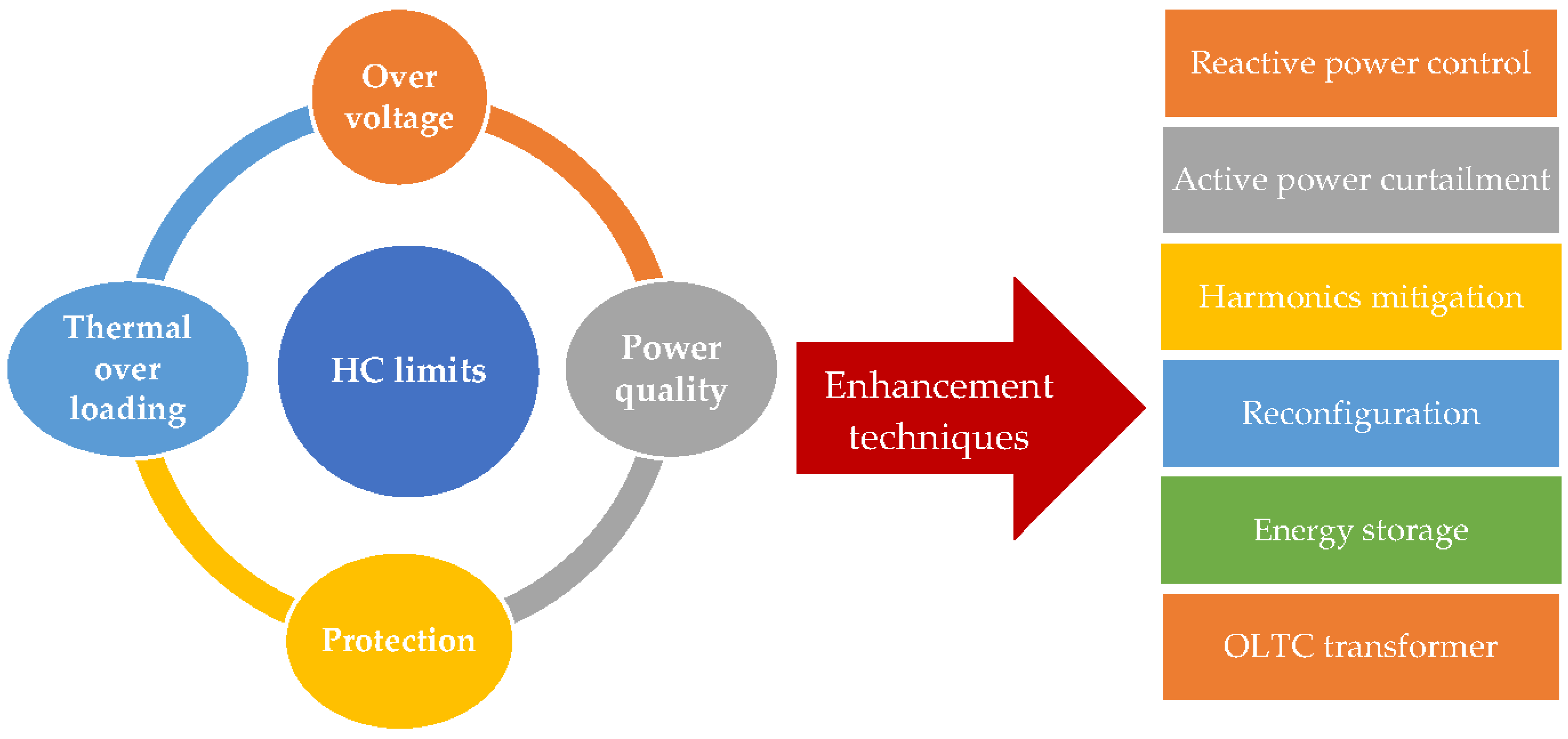
1.1. Background and Motivation

Recently, renewable and sustainable energy sources (RSESs) have been widely used to cope with the increase in global energy consumption and environmental pollution. According to the authors of [1], it is expected that the electricity generation from renewables will increase to 23,477 Billion KWh by 2050 to reduce the reliance on fossil fuel-based generation units. Incorporating the RSESs into modern power systems minimizes the systems’ security and increases the hazards [2]. The output of RSESSs is unpredictable, and the enormous use of RSESs increases the power systems’ uncertainties. Unplanned integration of RSESs increases the power system losses, overloading of power system’s components, and reliability issues such as exceeding the limits of short circuit capacity [3]. It may lead to partial or complete electricity outages.

Several research studies have been conducted to enhance the hosting capacity (HC) of modern power systems. HC studies aim to maximize the generation from RSESs that can be hosted in power systems without violating the operational constraints [4,5]. The HC has adverse impacts such as over-voltage, power losses, overloading, power quality, and protection problems, as explained in Figure 1 [4]. A voltage rise occurs if the output of the distribution generation units (DGs) exceeds the load demand and the surplus power flows to the network. Inaccuracies in locating DGs may result in reverse power flow to the upstream network that may surpass the thermal capacity of transmission lines and increase power losses. The massive use of DGs increases the power system harmonics and voltage dips and flickers. Moreover, it affects the magnitude and direction of the fault currents’ direction and magnitude that cause many protective issues.

Many techniques are have been suggested to mitigate the undesirable impacts of HC, as described in Figure 1 [4]. Simultaneous incorporation of RSESs, energy storage systems (ESSs), and reactive power sources was proposed by Santos et al. [6] and Santos et al. [7] to maintain the buses’ voltage within their limits and control reactive power. The impact of the on-load tap changer (OLTC) and the control of reactive power was proposed by Bletterie et al. [8] to compensate for the voltage of networks and enhance the HC automatically. The active power curtailment of DGs and the use of ESSs were introduced by Etherden et al. [9] and Etherden et al. [10], respectively, as effective tools to increase the HC of networks through balancing the mismatch between the generation and the consumption and tackling overvoltage and overloading issues. The impact of network reinforcement on supporting HC was studied by Navarro-Espinosa et al. [11]. The results revealed that it was cost-effective for low HC levels. Harmonic distortion constraints were embedded with the model suggested by Sakar et al. [12]. It was shown that the non-sinusoidal system’s voltage distortions and the load’s nonlinearity degree significantly impact the level of HC.

Increasing the HC in the planning phase is an alternative and effective way to overcome the shortcomings brought out from the massive use of RSESs. There is still much effort to provide a planning model capable of increasing the HC and avoiding the problems mentioned earlier.

1.2. Literature Review

In power system planning (PSP), power systems operators and planners define the optimal places and numbers of new generation stations, transmission circuits, or any other facility needed for expanding existing power networks to meet future load demands and fulfill security and reliability requirements [13]. PSP also decides the location and the size of other facilities such as fault current limiters, thyristor control series compensators, and ESSs if the candidate lines and generation units technically do not achieve the security and reliability constraints. These facilities are also used when they are economically favorable compared to the new circuits and generation units [14,15].

Four factors are affecting the accuracy of PSP. The first factor is the planning model. It can be a DC or AC optimal power flow-based model [16]. The AC model is more accurate compared with the DC model; however, it needs a higher computational burden [17,18,19].

The second factor is solution methods. Mathematical, heuristic, and meta-heuristic techniques are widely used to solve PSP problems. The mathematical approaches are effective to solve linear and simple problems, but they need higher computational efforts for solving problems with large search space [20,21,22]. The heuristic methods give high-quality solutions, but they cannot guarantee optimal solutions [23,24]. The meta-heuristic techniques need lower computational efforts than the mathematical techniques and are recommended for solving non-linear large-scale optimization problems [17,25,26,27,28]. The main disadvantage of meta-heuristic techniques is that they must be carried out for several runs to reach optimal solutions. Recently, many studies have tended to combine the characteristics of several meta-heuristic methods in a single algorithm with the hope of capturing high-quality solutions. Eslami et al. [29] suggested a hybrid algorithm based on a chaotic sine cosine algorithm and pattern search. The hybrid algorithm showed its superiority compared to some techniques from the literature in solving a set of benchmark problems. Neshat et al. [30] proposed a multi-swarm cooperative co-evolution framework. It comprised three meta-heuristics with a backtracking approach to speed up the optimization process and enhance the obtained solutions. The hybrid particle swarm algorithm with sine-cosine acceleration parameters was introduced by Chen et al. [31] to tackle the particle swarm algorithm’s shortcomings. The results proved the efficiency of the proposed approach.

The third factor is the type of reliability constraint. N-1 security and short-circuit current (SCC) limitations are the most applied to preserve the systems’ reliability in the planning phase [3,21,32]. Power systems must be ready to feed loads to any emergency that leads to a single generation unit or a transmission circuit being out of service. The short circuit current must be lower than the permissible levels to avoid the replacement of the installed circuit breakers.

The fourth factor is the approach applied to handle the power system’s uncertainties. As stated before, the output of RSESs is unpredictable, and the load demands change randomly, which increases the systems’ stochasticity. Many studies have been carried out to deal with this problem [33,34]. The stochastic and robust approaches are commonly applied to consider uncertainties in the PSP problem. The stochastic approach utilizes the proper probability distribution function for each uncertain variable to simulate its variation; however, the upper and the lower boundaries of the variables are sufficient for the robust approaches to consider uncertainties [35,36].

Several planning models have been presented to increase the use of RSESs and reduce carbon dioxide emissions in the planning phase; however, the available literature is still lacking to investigate a model that measures to what extent the networks can host RSESs [13].

Table 1. Summary of related works.

Ref.	Planning Model	The Methodology Applied for Integration RSESs
Refaat et al. [3]	A stochastic PSP model considering SCC constraints and N-1 security was adopted.	Economic and technical requirements constrained the penetration level of renewable units.
Luburić et al. [19]	An investment model aimed to find the optimal mix of transmission lines, TCSCs, and ESS was proposed.	Renewables’ maximum level was decided before conducting the analysis.
Hamidpour et al. [20]	A stochastic planning strategy to coordinate GEP, TEP, and ESSs expansion planning in the presence of demand response was established.	The expansion cost of RSESs was embedded in the objective function.
Gan et al. [22]	A security-constrained co-planning model of TEP and ESSs with high penetration of RSESs was presented.	The risk cost due to Renewable curtailed was presented in the cost function.
Najjar et al. [32]	A simultaneous model for GEP and TEP that considers SCC constraints was presented.	The expansion cost of RSESs controlled the use of RSESs.
Zhou et al. [37]	A precise PSP method was established to evaluate the operating costs involving robust hourly transmission constrained unit commitment and economic dispatch problems.	The penetration level of renewable units hosted was restricted by the economic costs and the technical aspects.
Zhang et al. [39]	An innovative scenario-based model that incorporated GEP, TEP, and reactive power planning problems was formulated.	A penalty cost due to Renewable curtailed was included in the objective function.
Mortaz et al. [40]	A TEP model was formulated to evaluate the impact of RSESs’ penetration level on TEP’s projects.	Defined RSESs’ capacity was distributed among different numbers of buses to assess the impact of use RSESs on TEP cost and projects required.
Zhuo et al. [41]	A Stochastic TEP planning model was established to consider enormous scenarios without employing a reduction method.	Different RSESs’ penetration levels were suggested to evaluate the proposed methodology.
Akhavizadegan et al. [42]	A bi-level optimization model was designed, and a new approach was proposed to identify a small number of high-quality scenarios for TEP.	The proposed method was investigated assuming that renewable energy capacity would increase by a fixed ratio each year until the end of the planning horizon.

summarizes some of them. Zhou et al. [37] presented a new PSP method for wind farms and ESSs considering the multi-stage operation process of networks. A parallel horizon-splitting method and a new genetic algorithm nested gradient descent technique were investigated to solve the problem. Abushamah et al. [38] proposed a novel strategy for formulating the composite centralized and distributed GEP problem to find the capacity, technology, operation strategy and optimal location of non-stochastic DGs. The genetic algorithm was employed to solve the problem.

Further, Zhang et al. [39] introduced an innovative scenario-based stochastic model for PSP that integrates reactive power planning. It considered the spinning reserve, unit ramp rate, and output of generation units. A relaxed AC optimal power flow was used to consider reactive power flow and buses’ voltage and angle constraints. Unit status and transmission switching were also applied to increase wind power usage and enhance the power system reliability. Mortaz et al. [40] studied the effect of RSESs on the TEP. The hourly resolution for RSESs and load demand were considered to study the impacts of correlation of capacities, fluctuations, variable resources, and locations on the TEP’s projects. A meta-heuristic technique named binary particle swarm optimization was adopted to solve the problem.

A massive scenarios-based model without implementing a reduction method was adopted in Zhuo et al. [41]. The TEP problem was divided into a master problem and several sub-problems. A strategy was proposed to reduce computation time. Akhavizadegan et al. [42] proposed a new approach to reduce the number of representative scenarios. The results demonstrated that the TEP-based proposed approach was more accurate than the well-established selection techniques reported in the literature.

1.3. Novelty and Contribution

In this work, the HC planning model is proposed for supplying the future load demands, measuring to what extent the penetration of RSESs can reach in modern power systems, and ensuring technical constraints. A load forecasting technique, incorporated with the planning model, is also employed to predict the annual load growth. A hybrid optimization algorithm that combines the features of two meta-heuristic techniques is established to solve the problem and tackle the shortcomings of meta-heuristic techniques. The HC planning scheme suggested is conducted on two test systems. The main contributions of the paper can be summarized as follows:

• HC planning model, which increases the host of RSESs and meets the future load demands, is proposed.
• The objective function is investigated to be more concerned with facilities’ size and quantity than the investment cost. It is formulated to determine the size of the thermal units that can be replaced to reduce environmental pollution. In addition, it targets to find the optimal TEP projects and FCLs and ESSs’ place and size to increase the HC level and guarantee the SCC and N-1 constraints without needing load shedding.
• A load forecasting technique based on adaptive neural fuzzy systems (ANFIS) is applied to predict the expected load growth.
• The hybrid optimization algorithm of the weighted mean of vectors optimizer [43] and the sine cosine algorithm [44] (INFO-SCA) is adopted to solve the problem.

2. Problem Formulation

The proposed HC planning model is formulated to reduce the reliance on conventional power units and maximize the use of RSESs. It aims to decide the optimal location of ESSs and RSES units such that the TEP’s projects are reduced and N-1 and SCC securities are achieved. The problem of FCLs placement and sizing are included in the model to meet the SCC Reliability.

To handle the network’s uncertainties, the suggested model takes into account the variation of load demand and the wind speed over 48 h. Outputs of RSESs are calculated using data of the selected scenarios [45].

The DC model is adopted in this work to reduce the complexity of the problem. The PSP problem is formulated as an optimization problem with four sub-objective functions and a set of constraints. The HC planning model considering N-1 reliability and SCC constraint is described below.

2.1. Objective Function (OF)

The problem OF is illustrated in (1). It aims to maximize the usage of RSESs and determine the location of new circuits and the size and place of FCLs and ESSs needed. In addition, the OF reduces the required load shedding to meet N-0 and N-1 securities.

$$OF=min\left\{{\omega }_G C_{GEP}^G+{\omega }_l C_{TEP}^l+{\omega }_{FCL} C_{SCC}^{FCL}+{\omega }_{shed} C_{penalty}^{shed}\right\}$$

(1)

The OF consists of four sub-objectives, as follows:

$$C_{GEP}^G={\displaystyle \sum }_{i=1}^G{\displaystyle \sum }_{h=1}^T\frac{{\omega }_g{P}_{g,i}^S+ {\omega }_{ESS} P_{ESS,i}^S}{P_{g,i}^S+P_{R,i}^S+P_{ESS,i}^S}$$

(2)

$$C_{TEP}^l={\displaystyle \sum }_{S=1}^{S_{max}}{\displaystyle \sum }_{i=1,j=1,i\ne j}^{i = n,j=n,i\ne j}\frac{C_{ij}(N_{ij}{}^S-N_{ij}{}^{S-1})}{C_{ij}(N_{ij}{}^{S,max}-N_{ij}{}^{S-1})}$$

(3)

$$C_{SCC}^{FCL}=\frac{{{\displaystyle \sum }}_{i=1}^{N_{FCL}}{{\displaystyle \sum }}_{S=1}^{S_{max}}{x}_{FCL,i}^S}{{{\displaystyle \sum }}_{i=1}^{N_{FCL}}{x}_{FCL,i}^{max}}$$

(4)

$$C_{penalty}^{shed}={\displaystyle \sum }_{i=1}^n{\displaystyle \sum }_{S=1}^{S_{max}}\frac{P_{shed,i}^s}{P_{d,i}^{s,max}}$$

(5)

The increase in the hosting capacity is achieved by minimizing the ratio between the output of thermal units and ESSs concerning the outcome of the RSESs, as explained in (2). The proposed model strives to reduce reliance on ESSs as possible. According to (2), $C_{GEP}^G$ equal or greater than ${\omega }_g$ means no RESs are installed, while $C_{GEP}^G$ of a zero value means that RSESs replace the existing thermal units, and no ESSs are needed. In (2), the objective is to install as many RSESs as possible regardless of the cost. ${\omega }_g$ and ${\omega }_{ESS}$ are weighting factors selected to guarantee that minimizing the output of thermal units is the priority. The second term in (1) explores the optimal location of TEP’s projects as described in (3). The cost of TEP’s projects is normalized such that the output of (3) does not exceed 1 and matches with the output of (2). The third term in the OF optimizes the location and the size of FCLs to maintain the SCC blew the rated value. Similar to (3), equation (4) is normalized such that the output is between 0 and 1. ${\omega }_l$, ${\omega }_G$, ${\omega }_{FCL}$, and ${\omega }_{shed}$ are weighting factors.

As mentioned in [3], achieving N-1 security in some networks needs the application of forced load shedding. The candidate circuits and the other candidate facilities may not ensure the N-0 and N-1 securities. Therefore, the OF is extended to minimize the required load shedding to realize the system’s reliability. The fourth term in (1) is zero if no load shedding is required and increases up to one if load shedding is a must.

Regarding (3), the circuits’ cost ($C_{ij}$) are needed because they depend on the length and the capacity of the circuits. However, the cost of FCLs is neglected in (4) because the cost of FCLs is a function of the size of FCL ($x_{FCL}$), hence $x_{FCL}$ is only necessary for the normalized formula.

It is shown that the penetration level of RSESs no longer depends on their economic feasibility, and increasing the HC is the first task. The four coefficients ${\omega }_l$, ${\omega }_G$, ${\omega }_{FCL}$, and ${\omega }_{shed}$ are introduced to control the problem objectives. For example, if the priority for the system’s planner is to study the impact of the use of RSESs on TEP projects, ${\omega }_l$ will be selected to be larger than other variables.

The suggested model becomes flexible by introducing the governor variables ${\omega }_g$ and ${\omega }_{ESS}$. By controlling these variables, the planner can decide which facility will compensate for unbalancing between the generation from RSESs and the consumption. If ${\omega }_{ESS}$ is larger than ${\omega }_g$, this implies that thermal units are responsible for compensating for a deficiency in renewable power.

2.2. Problem Constraints

The suggested optimization problem is subjected to a set of constraints provided in (6)–(23). Equations (6)–(18) describe the normal operation constraints, while congestion relief constraints are shown in (19)–(23).

2.2.1. Normal Operation Constraints

In the normal operation, the HC planning problem is constrained by active power balance equilibrium at each bus, lines’ thermal limits, voltage regulation bounds, and facilities capabilities. The active power equilibrium restriction, provided in (6), ensures that the power injected at scenario S at node i equals the difference between the total generated power at bus i, including the power discharged from ESSs and the power consumed at bus i due to electrical load and ESSs’ power charged. The power flow constraint is defined in (7). It maintains the power flows in the circuits between nodes i and j below the maximum level.

$$P_{g,i}^S+P_{R,i}^S-P_{d,i}^S+P_{shed,i}^S+P_{ch,i}^S+P_{dch,i}^S={\displaystyle \sum }_{\begin{array}{c}i,j\in N\\ i\ne j\end{array}}{P}_{ij}^S$$

(6)

$$-P_{ij}^{max}\le {\beta }_{ij} N_{ij}{}^S \left({\theta }_i^s-{\theta }_j^s\right)\le P_{ij}^{max}$$

(7)

The box-type constraints (8)–(12) restrict buses’ voltage angle, installed circuits, load shedding, and the outputs of RSESs and thermal units within their limits. They must not exceed the maximum permissible limits. The constraint (9) enforces that circuits constructed at previous scenarios exist in the next scenarios.

$${\theta }_i^{min}\le {\theta }_i^S\le {\theta }_i^{max}$$

(8)

$$N_{ij}^{S-1}\le \left(N_{ij}{}^{new,S}\right)\le N_{ij}^{max}$$

(9)

$$0\le P_{shed,i}^S\le P_{d,i}^{max,S}$$

(10)

$$P_{R,i}^{min}\le P_{R,i}^S\le P_{R,i}^{max}$$

(11)

$$P_{g,i}^{min}\le P_{g,i}^S\le P_{g,i}^{max}$$

(12)

Constraints (13) and (18) are related to the operation of ESSs installed. Inequality constraint (13) limits the maximum number of ESSs built at each scenario. While the box-type restrictions (14) and (15) controls charging power and discharging power of ESSs at each node. They must not be more than the rated values. Constraints (16)–(18) enforce that the state of charge and capacity of ESS built do not violate the upper and lower bounds.

$$N_{ESS,i}^{S-1}\le N_{ESS,i}^S\le N_{ESS,i}^{max}$$

(13)

$$0\le P_{dch,i}^S\le P_{dch,i}^{max}$$

(14)

$$0\le P_{ch,i}^S\le P_{ch,i}^{max,S}$$

(15)

$$SO{C}_{ESS,i}^{min}\le SO{C}_{ESS,i}^S\le SO{C}_{ESS,i}^{max}$$

(16)

$$0\le E_{ESS,i}^S\le E_{ESS,i}^{max}$$

(17)

$$SO{C}_{ESS,i}^S=SO{C}_{ESS,i}^{S-1}+{\eta }_{ESS}^{ch}{P}_{ch,i}^S-\raisebox{1ex}{$P_{dch,i}^S$}\!\left/ \!\raisebox{-1ex}{${\eta }_{bat}^{dch}$}\right.$$

(18)

2.2.2. Congestion Relief Constraints

The congestion relief constraints, N-1 security, and short-circuit current restriction are explained in (19)–(23) [3]. Restrictions (19) and (20) guarantee, for a single line outage contingency, the capability of installed devices to meet the power balance equilibrium, and lines’ thermal limit constraints. Transmission lines’ contingencies are only integrated into the model because they frequently occur compared with generation units’ contingencies.

$$P_{g,i}^S+P_{R,i}^S-P_{d,i}^S+P_{shed,i}^S-P_{ch,i}^S+P_{dch,i}^S={\displaystyle \sum }_{\begin{array}{c}i,j\in N\\ i\ne j\end{array}}{P}_{ij}^S$$

(19)

$$-P_{ij}^{max}\le {\beta }_{ij}(N_{ij}{}^S-1) \left({\theta }_i^S-{\theta }_j^S\right)\le P_{ij}^{max}$$

(20)

The three-phase fault is the worst and commonly occurs in power systems; hence it is considered. Short circuit current constraints are expressed in (21)–(23). The box-type Equation (21) defines the size of FCLs required to control the maximum fault current, while constraints (22) and (23) maintain the fault current below the maximum permissible limit.

$$N_{ij}{}^{s-1}{x}_{ij}^{FCL,s-1}\le x_{ij}^{FCL,s}\le N_{ij}{}^{new,s}{x}_{ij,max}^{FCL}$$

(21)

$$I_i^{SC,s}\le I_{max}^{SC}$$

(22)

$$I_i^{SC,s}=\frac{V_i\left(0\right)}{Z_{ii}}$$

(23)

2.3. Economic Analysis

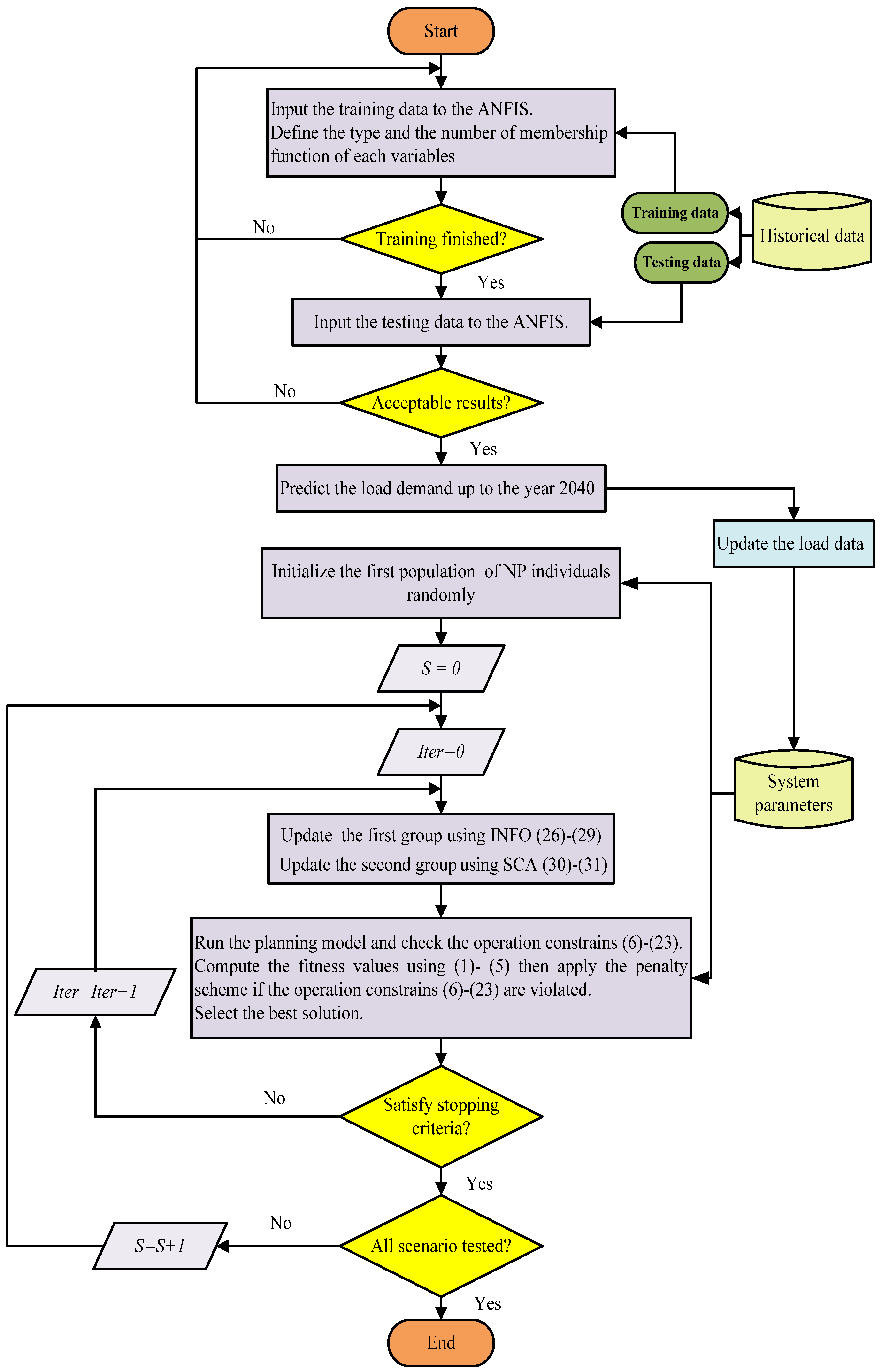
Levelized cost of energy (LCOE) is applied to measure the effectiveness of installed projects compared to other facilities. It is computed in $/MWh as given in (24) [46,47].

$$\mathrm{LCOE}=\frac{RF\times \left(C_{invest}^l+C_{cap}^R+C_{op}^R+C_{cap}^g+C_{op}^g+C_{cap}^{ESS}+C_{op}^{ESS}+C_{cap}^{FCL}\right)}{{{\displaystyle \sum }}_{S=1}^T{E}_s^R}$$

(24)

$C_{invest}^l$ is the cost of new circuits. $C_{cap}^R$, $C_{cap}^g$, $C_{cap}^{ESS}$, and $C_{cap}^{FCL}$ are the capital costs of new RSESs, thermal units, ESSs and FCLS. While $C_{op}^R$, $C_{op }^g$, and $C_{op}^{ESS}$ are the operational costs of RSESs, thermal units, and ESSs. RF is the recovery factor and is calculated as follows:

$$RF=\left(\frac{\lambda {\left(1+\lambda \right)}^y}{{\left(1+\lambda \right)}^y-1}\right)$$

(25)

where $\lambda$ and $y$ are discount rates and the planning horizon.

3. Methodology

A hybrid of INFO and SCA is investigated in this work to solve the suggested problem. The load forecasting process is inherent to the PSP. Therefore, the load forecasting based-ANFIS is incorporated with INFO-SCA to predict the annual load growth. A stochastic approach is applied to deal with uncertainties in power networks. A total of 48 data sets were collected to represent the variation of RSESs and electrical loads over two days. The main steps of the proposed strategy are summarized in Figure 2 and are explained in the following sub-sections.

3.1. Load Forecasting

Several techniques have been employed for long-term load prediction. The load forecasting-based ANFIS was selected and applied in this work. ANFIS can precisely predict the annual load growth and gives better results than some mathematical techniques [27,48].

ANFIS is widely used for solving many engineering problems. It combines the characteristics of artificial neural networks and fuzzy inference systems. ANFIS can capture the process’s non-linear structure, adaptability, and rapid learning capacity. However, it has a high computational cost, and its performance is constrained by the type and number of membership functions and the curse dimensionality [49].

ANFIS is implemented for load forecasting as described in Figure 2 [48]. It starts with defining the number of input variables and output variables. The ANFIS has a single input and a single output in this work. The input is the historical years, and the output is the peak load demand. The historical data set is divided into 70–90% training data and 10–30% testing data. After that, the number of fuzzy rules and the type of membership functions are decided. The training and testing processes are carried out to select the best model. Finally, the selected model is used to predict the future load demands.

3.2. Optimization Methods

INFO and SCA are two meta-heuristic optimization techniques and were firstly developed by Ahmadianfar et al. [43] and Mirjalili et al. [44], respectively. They present a good performance in solving many non-linear large-scale optimization problems. Like any meta-heuristic algorithm, they must be conducted for several runs to reach the optimal solution. The main features of both algorithms are outlined in

Table 2. Comparative analysis of INFO and SCA.

Features	INFO [43]	SCA [44]
Mechanism of operation	It is based on the idea of weighted means of vectors. The updating process is done in three stages: updating rule, vector combining, and a local search.	The updating process is based on sine and cosine functions to vary the candidate solutions either outwards or towards the best solutions.
vantages	It is efficient in solving real complex and challenging problems. It is capable of avoiding local optimums and converges fast to optimal solutions.	It is superior in solving unimodal, multi-modal, and composite test functions compared to some algorithms reported in the literature. It is recommended for solving complex engineering problems.
Limitations	Like any meta-heuristic technique, INFO and SCA do not guarantee the optimum solutions. Further, for both optimizers, well-defined algorithm parameters for one problem may not be suitable for solving another problem.

.

In this study, both algorithms were combined to solve the proposed problem. The hybrid of INFO and SCA (INFO-SCA) is suggested to improve the exploration and exploiting phases to get high-quality solutions with a minimum number of iterations and runs.

The procedure applied to solve the PSP problem is given in (26)–(31) and is detailed in Figure 2. The operational mechanism of the INFO-SCA can be summarized in the following steps:

Step 1:

The initial population is randomly generated considering the lower and upper bounds of the decision-making variables.

Step 2:

The population is divided into two groups. The first group contains the first half of the population, and the new variables are obtained using INFO’s updating scheme provided in (26)–(29). The updating scheme is carried out in three stages: updating rule, vector combining, and a local search. The first stage enhances the diversity of the population during the search procedure, as illustrated in (26) and (27).

$$po{p}_1^{stage1}=\{\begin{array}{c}po{p}^t+\sigma \times meanrule+rnd\times \frac{po{p}^{bs}-po{p}^{a1}}{f\left(po{p}^{bs}\right)-f\left(po{p}^{a1}\right)+1}, if rand<0.5\\ po{p}^a+\sigma \times meanrule+rnd\times \frac{po{p}^{a2}-po{p}^{a3}}{f\left(po{p}^{a2}\right)-f\left(po{p}^{a3}\right)+1}, if rand\ge 0.5\end{array}$$

(26)

$$po{p}_2^{stage1}=\{\begin{array}{c}po{p}^{bs}+\sigma \times meanrule+rnd\times \frac{po{p}^{a1}-po{p}^b}{f\left(po{p}^{a1}\right)-f\left(po{p}^b\right)+1}, if rand<0.5\\ po{p}^{bt}+\sigma \times meanrule+rnd\times \frac{po{p}^{a1}-po{p}^{a2}}{f\left(po{p}^{a1}\right)-f\left(po{p}^{a2}\right)+1}, if rand\ge 0.5\end{array}$$

(27)

$po{p}^{bt}$ and $po{p}^{bs}$ are the better and best solutions in the population, respectively. The better solution is randomly selected from the top five solutions. $po{p}^{a1}$, $po{p}^{a2}$, and $po{p}^{a3}$ are randomly selected from the population.$f\left(pop\right)$ is the fitness value of $pop$ solution. $rnd$ is a random number between 0 and 1. $meanrule$ is calculated as explained in [43].

The second stage promotes the local search ability to give promising solutions, as shown in (28).

$$po{p}^{stage2}=\{\begin{array}{c}po{p}_1^{stage1}+\mu . \left|po{p}_1^{stage1}-po{p}_2^{stage1}\right|, if rand1<0.5 and rand2<0.5\\ po{p}_2^{stage1}+\mu . \left|po{p}_1^{stage1}-po{p}_2^{stage1}\right|, if rand1<0.5 and rand2\ge 0.5\\ po{p}^t, if rand1\ge 0.5\end{array}$$

(28)

$po{p}^{stage2}$ is the output vector in the second stage, and $\mu$ equals 0.05 × rnd.

The third stage is investigated to avoid dropping into local optimums as follows:

$$po{p}^{t+1}=\{\begin{array}{c}po{p}^{bs}+rnd \times \left(meanrule+rnd\times \left(po{p}^{bs}-po{p}^{a1}\right)\right), \\ if rand3<0.5 and rand4<0.5\\ po{p}^{rnd}+rnd \times \left(meanrule+rnd\times \left(v_1\times po{p}^{bs}-v_2\times po{p}^{rnd}\right)\right),\\ if rand3<0.5 and rand4\ge 0.5\\ po{p}^{stage2}, if rand3\ge 0.5\end{array}$$

(29)

$po{p}^{rnd}$ is a new solution that combines the solutions $po{p}^{avg}$, $po{p}^{bt}$, and $po{p}^{bs}$. $v_1$ and $v_2$ are two random numbers. More details about INFO are presented in Ahmadianfar et al. [43].

Step 3:

The second group comprises the second half of the population, and the SCA is employed to update the decision-making variables. The SCA’s updating scheme is explained in (30) and (31).

$$po{p}^{t+1}=\{\begin{array}{c}po{p}^t+R_1\times \sin \left(R_2\right)\left|R_3\times po{p}^{bs}-po{p}^t\right|, if R_4<0.5\\ po{p}^t+R_1\times \cos \left(R_2\right)\left|R_3\times po{p}^{bs}-po{p}^t\right|, if R_4\ge 0.5\end{array}$$

(30)

$R_1$ changes in each iteration using (31). $R_2$, $R_3$, and $R_4$ are randomly selected.

$$R_1=a-\frac{iter}{ite{r}_{max}}$$

(31)

where $ite{r}_{max}$ is the maximum number of iterations, and a is a constant. Further information about SCA can be obtained in the prior work of Mirjalili et al. [44].

Step 4:

After each iteration, the objective functions are calculated after the new variables in each group are obtained. If the candidate solutions do not meet the operating constraints, a high penalized value is added to the objective functions.

Step 5:

The solution, corresponding to the minimum fitness value in both groups, is regarded as the best solution, and in the next iteration, is used to calculate the new variables in the groups.

The suggested INFO-SCA exploits the advantages of both algorithms to enhance the performance and reduce the computational burden by reducing the number of required runs.

4. Numerical Results

The realistic Egyptian extra-high voltage network (EHVN) and the benchmark IEEE 24-bus system were selected for conducting the proposed study. The simulations were carried out on MATLAB r2021a platform via a DELL PC, with a model name of OptiPlex7050, having an Intel^® Core™ i7′ CPU at 2.6 GHz-16 GB RAM. The results were obtained over 30 separate runs to identify the best solutions.

4.1. Test Systems

The EHVN is a 500 kV network. It comprises 8 generating units, 17 loads, and 19 transmission lines, as described in Figure 3 [27]. Regarding the potential transmission projects, it was supposed that the maximum number of circuits is four to reinforce the network to host more RSESs and supply the demand centers in the period between the year 2020 and the year 2040. The data of the transmission lines, generations, and loads of EHVN are presented in Fathy et al. [27]. To increase the dependency on RSESs, it was suggested that buses 1, 5, 14, 17, and 18 were the candidate locations for new wind units. The rated capacity of each unit was 10 GW. It was assumed that buses 9, 15, 17, and 18 were suitable for linking with ESSs. The wind speed data and the peak load’s variation are adapted from [50,51], respectively. The testing scenarios are shown in Figure 4. The rated power and storage capacities of ESSs were 200 MW and 500 MWh. The maximum number of ESSs at each location is five. Noteworthily, ${\omega }_l$, ${\omega }_G$, ${\omega }_{FCL}$, and ${\omega }_{shed}$ were selected to be 0.2, 0.6, 0.2, 0.2, respectively. Whilst ${\omega }_g$ and ${\omega }_{ESS}$ were 1.75 and 0.25, respectively.

This study assumed that the EHVN supplies about 24.9% of electrical loads in Egypt. Hence, the historical data of the peak load demand in Egypt from 2008 to 2020 were selected to predict the annual load growth until 2040.

The IEEE 24 bus system is a well-done test system. The total power demand is 2850 + j 580 MVA. The locations of generation and demand centers are shown in Figure 5. Some modifications were carried out to make contingencies [52]. The new candidate routes are represented by dash lines, as seen in Figure 5, and the complete data of the system are introduced in [52]. It was suggested that the maximum number of circuits that could be installed in each route is 2. To increase the usage of RESs, it was assumed that buses 1, 13, and 23 were vital locations to install new wind units and replace the existing thermal units. The rated capacity of each unit was 1000 MW. The candidate position of ESSs was at buses 1, 13, 17, 18 and 23.

4.2. EHVN’s Expansion

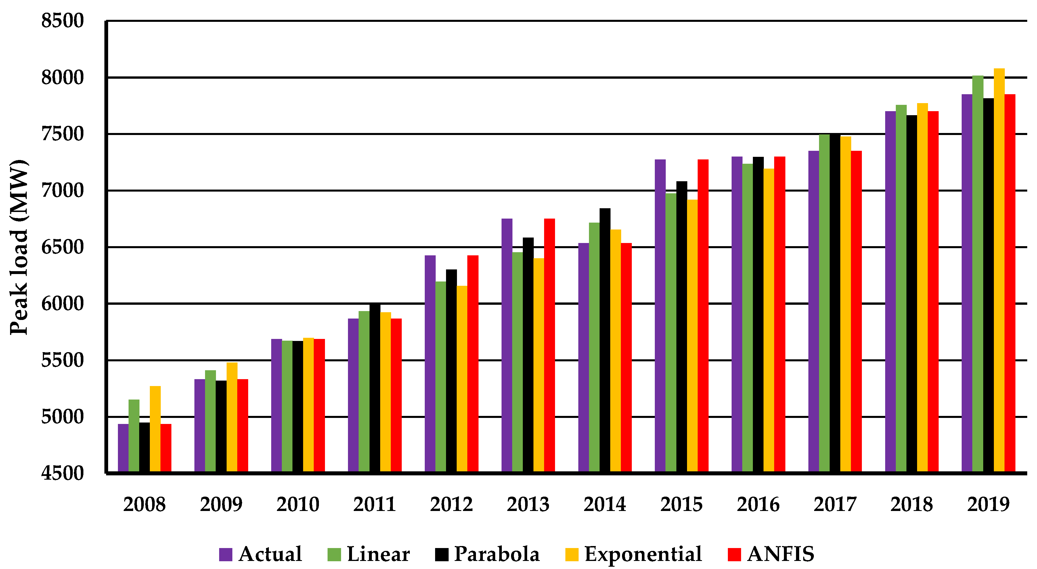
4.2.1. Load Forecasting for EHVN

A comparison between ANFIS-, linear-, parabola-, and exponential- based models for load forecasting is depicted in Figure 6. The historical data from the year 2008 to the year 2020 were used to investigate the performance of the four techniques. For ANFIS, the number of fuzzy rules was 15, and the number of nodes was 64. The historical data until the year 2019 were the trained data, and the data in 2020 were the tested data. As shown in Figure 5, although the test data has an upward trend, linear-, parabola-, and exponential- based models failed to forecast the peak loads precisely. The results demonstrated that the ANFIS was superior to other methods in terms of the sum of absolute error. It was 0.00061 for ANFIS and 151.57, 98.715, 181.83 and for linear-, parabola-, and exponential-based models, respectively.

Based on previous findings, the ANFIS was selected to predict the growth of loads up to the year 2040. As explained in Figure 7, the load will reach 27,716.3 MW in 2040. It was about 3.46 times the load in 2020. A lack of good planning to accommodate this stunning increase could threaten network security. In addition, reliance on conventional generation methods to meet the required consumption increases environmental pollution.

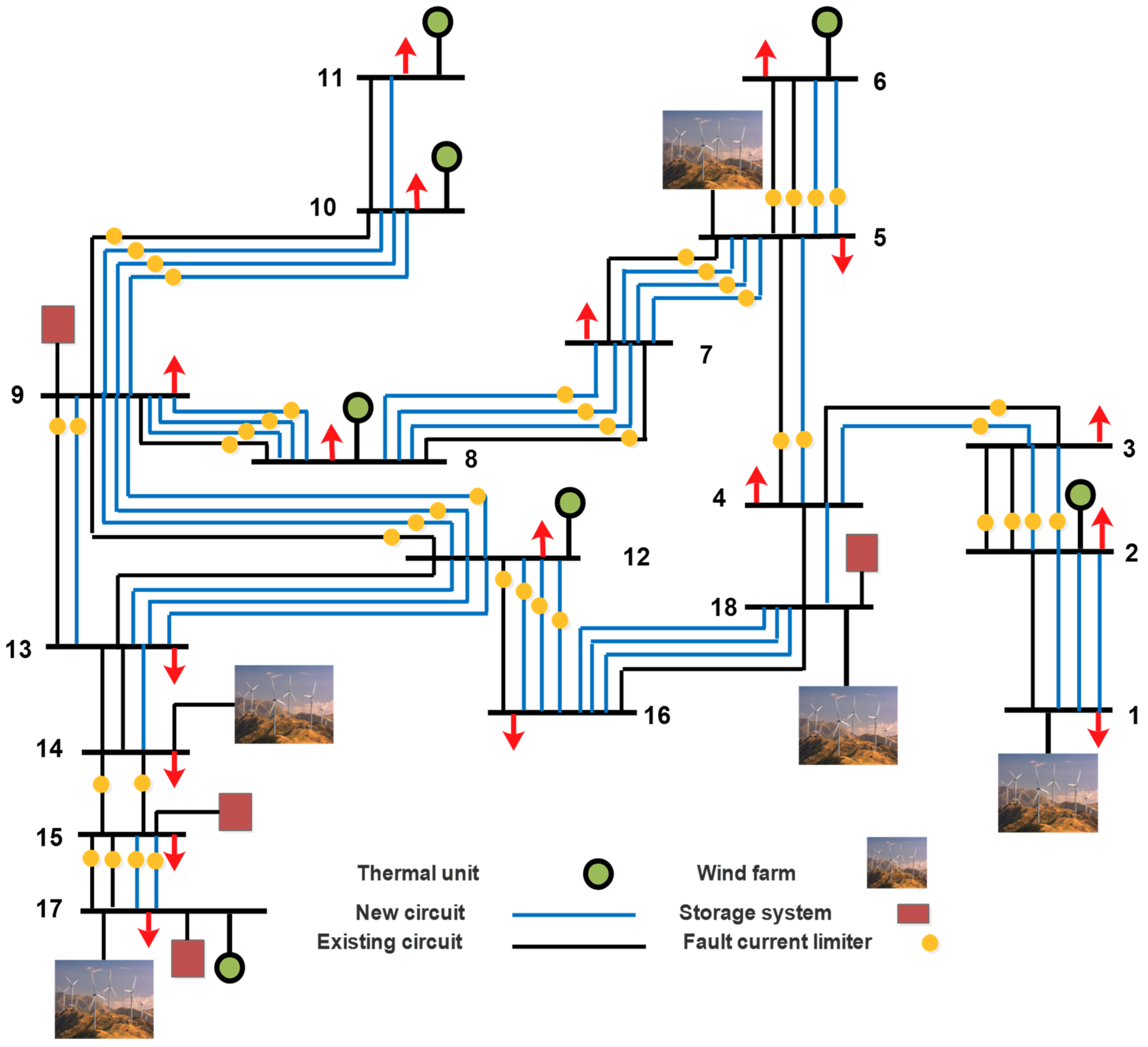
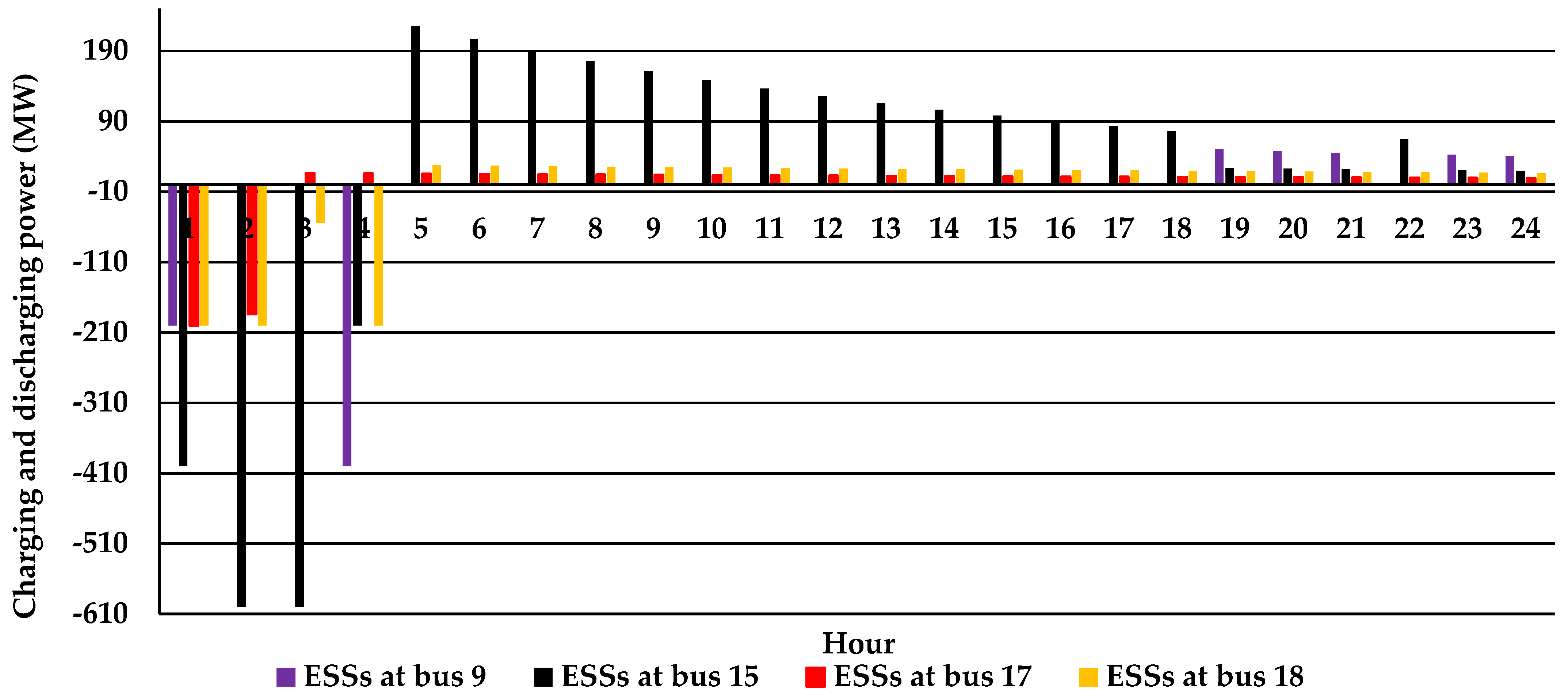
4.2.2. Configuration of EHVN in the Year 2040

Table 3. PSP’s projects for EHVN in the year 2040.

Route		No. Circuits	FCL Size	Bus	Total Generation (MWh)	ESS (MWh)
From	To
1	2	4	0	1	118,497.014 (wind)	0
2	3	4	4.163	2	6083.111 (thermal)	0
3	4	2	0.320	3	0	0
4	5	2	6.008	4	0	0
5	6	4	3.188	5	200,633.784 (wind)	0
5	7	4	0.426	6	18,031.351 (thermal)	0
7	8	4	6.112	7	0	0
8	9	4	5.938	8	16,489.200 (thermal)	0
9	10	4	6.032	9	0	3055.556
10	11	2	0	10	7344.435 (thermal)	0
9	13	2	3.099	11	5698.079 (thermal)	0
12	9	4	6.040	12	155,561.912 (thermal)	0
12	13	4	0	13	0	0
13	14	3	0	14	189,688.367 (wind)	0
14	15	2	6.040	15	0	8611.111
17	15	4	6.038	16	0	0
12	16	4	6.040	17	245,539.772 (wind, thermal)	2108.467
16	18	4	0	18	200,686.896 (wind)	3687.427
4	18	2	0

reveals the projects required for EHVN’s expansion. There was a need for 63 circuits to satisfy the demands needed at each hour. Blue lines in Figure 8 represent locations of new circuits. The results obtained showed that no load shedding was employed to achieve the reliability requirements.

The results also showed that the HC varies between 44.81% and 100% over the 48 scenarios, as shown in Figure 9. The maximum share of wind units was from scenario number 32 to scenario number 48 when the peak load changed from 79.69% to 91.25% of the total peak loads, and wind speed varied between 8.58 m/s and 12.76 m/s. While the minimum share was at scenario number 1 at the loading of 87.81% and wind speed of 5.26 m/s. Figure 9 clarifies that the HC increased in low consumption periods and high wind speed. Noteworthy, the wind farms at buses 1, 5, and 14 contributed about 13.022%, 22.042%, and 20.84% of the total output of RSESs, while wind units at buses 17 and 18 shared the same percentage of 22.048%.

As illustrated in Table 3, the optimal places for ESSs were at nodes 9, 15, 17, and 18. The total capacity of ESSs required was 17.462 GWh. It is divided as follows: 3.0556 GWh for the ESSs at bus 9, whereas the capacities of the storage systems at buses 15, 17, and 18 were 8.611 GWh, 2.108 GWh, and 3.687 GWh, respectively. The ESSs’ power needed over the first 24 h is described in Figure 10. The major reliance on ESSs was at hours from 12 a.m. to 3 a.m. The use of ESSs was essential to enhance the HC and maintain the resilience of modern power systems. It is worth mentioning that the ESSs were forced to stop discharging power to the grid if the available power from RSESs is about 65% of the total loads at each hour. This condition was applied to allow the ESSs to charge in periods that outputs of wind units are high. The increase in the number of representative days may positively impact the level of ESSs shared.

Figure 11 illustrates the SOC of ESSs at buses 9, 15, 17, and 18 over the two representative days. The minimum SOC was about 90% at scenario 4 for the ESSs at bus 15, while it was about 97.5%, 98.4%, and 97.45% for ESSs at buses 9, 17, and 18. Although all ESSs did not reach the maximum discharge depth, it was not preferable to supply additional power to guarantee all storage systems were fully charged within two days.

Table 3 reflects that the use of FCLs was essential, and the dependency on the location and the number of new circuits, ESSs and generation units was not sufficient to achieve the short-circuit constraints. The locations of FCLs installed are shown in Figure 8 in yellow color. As shown in Figure 12, the maximum of short-circuit at each scenario did not exceed the maximum (62 p.u).

4.2.3. Impact of ${\omega }_g$ and ${\omega }_{ESS}$ on Expansion Projects

Figure 13 shows ESSs’ discharged power for the first three hours at different values of ${\omega }_g$ and ${\omega }_{ESS}$. As ${\omega }_{ESS}$ decreases and ${\omega }_g$ increases, the penetration of ESSs increases. Therefore, if ESSs need to be fully charged in a short period, it is preferable that ${\omega }_{ESS}$ is high to reduce energy discharged. These factors can also control ESSs if there are some issues related to the available area or the size of ESSs.

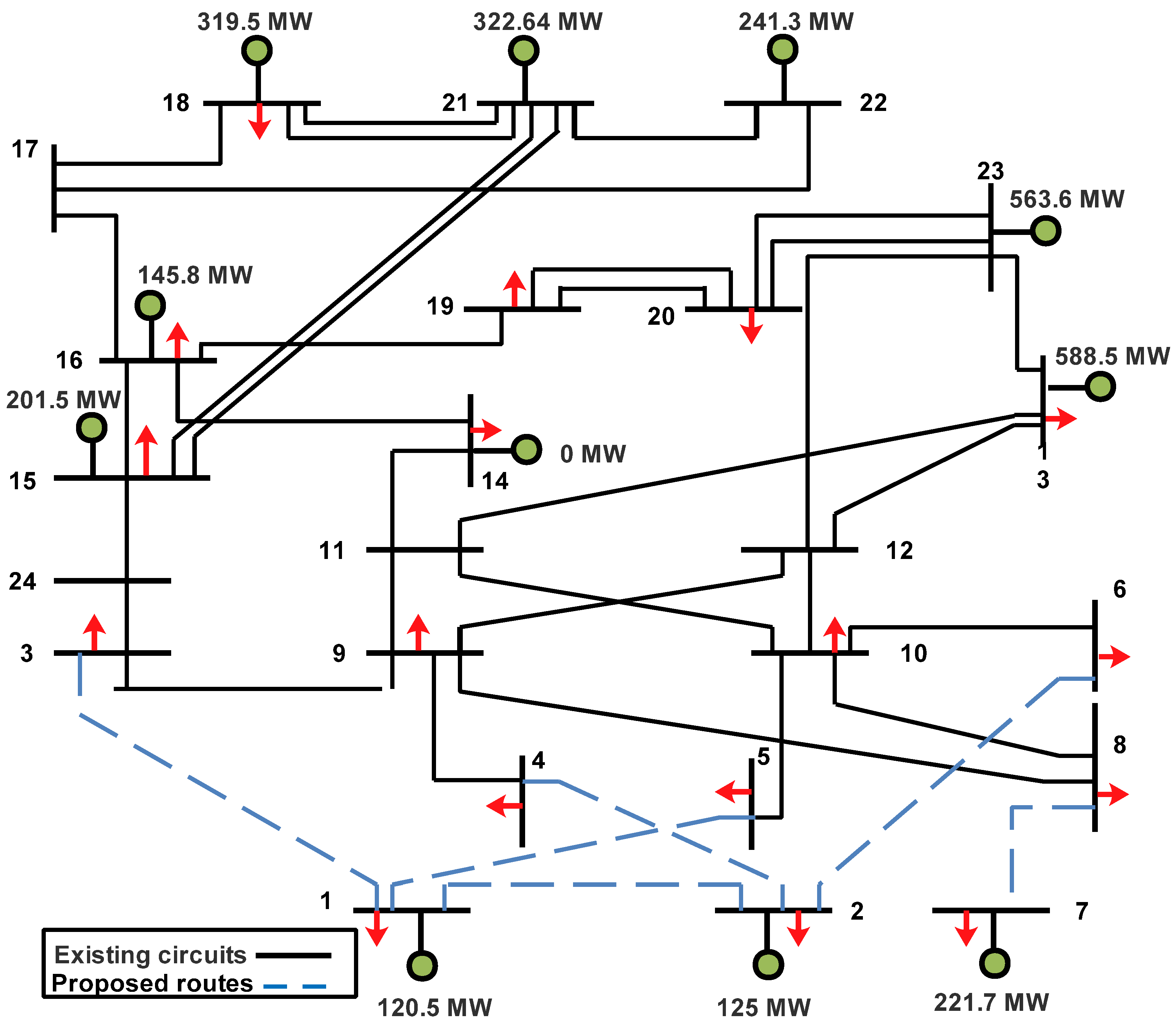
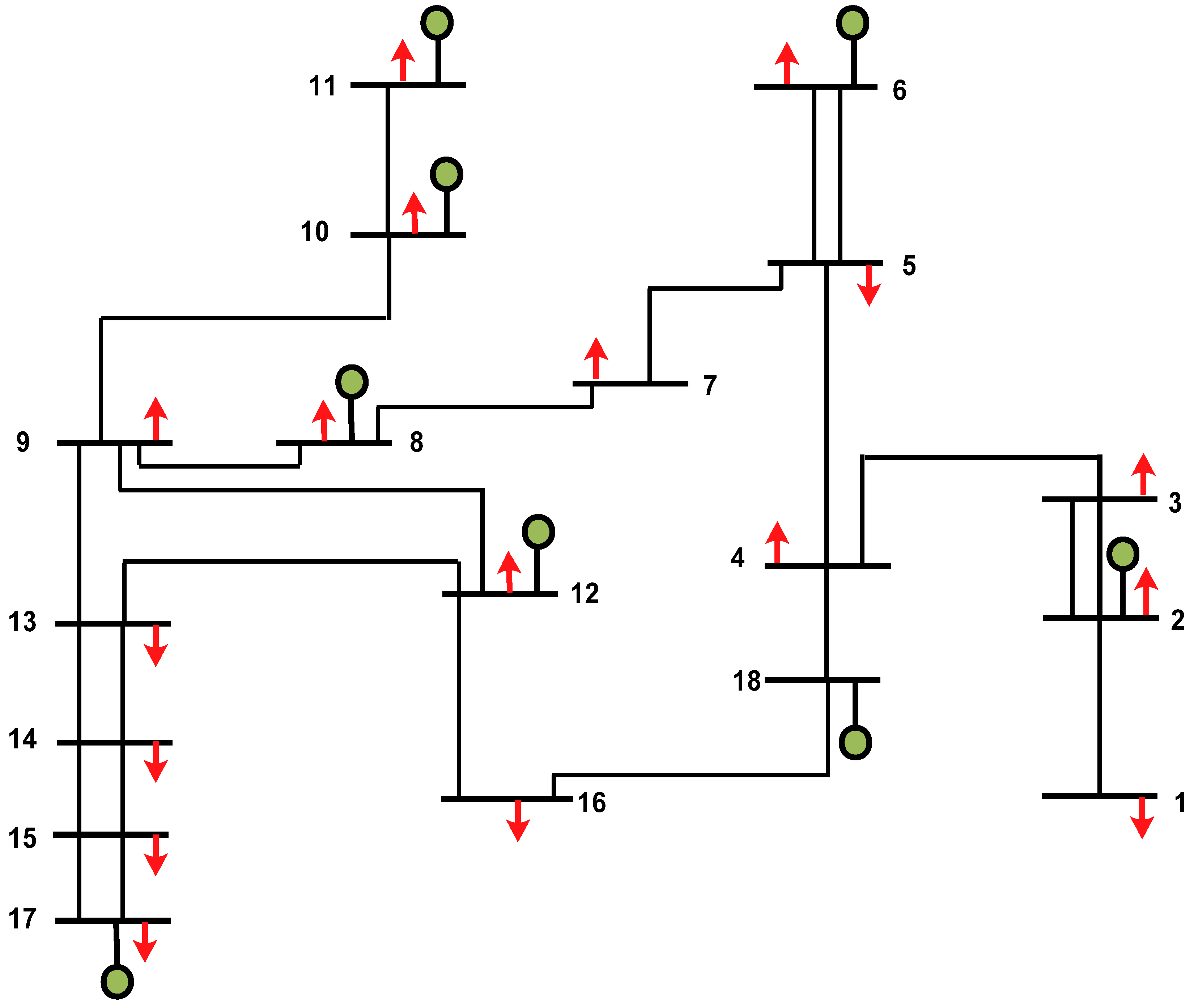
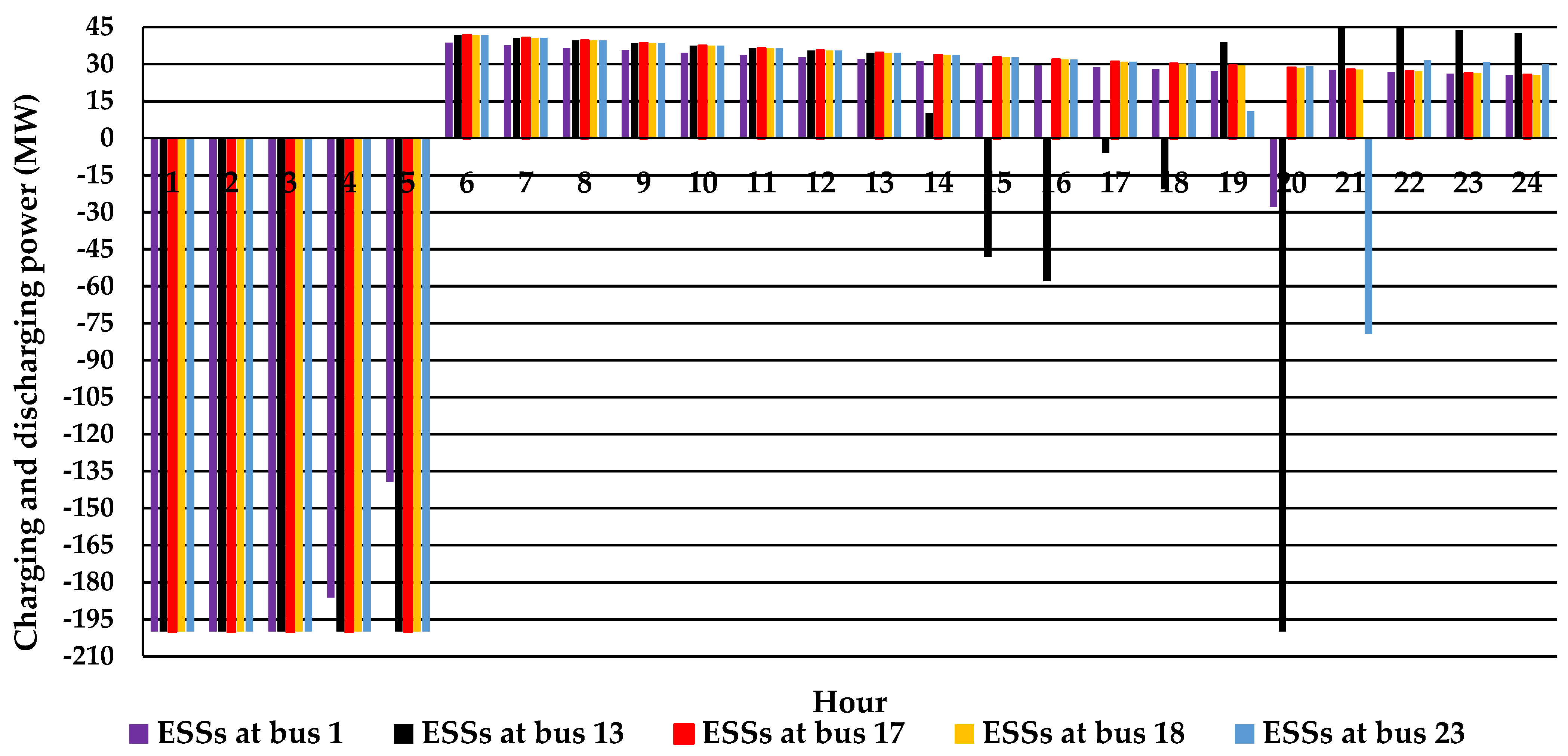
4.3. IEEE 24-Bus System’s Expansion

Final Configuration of the 24-Bus System

Figure 14 shows the final configuration of the 24-bus system. A total of 63 circuits were installed to achieve the reliability requirements, as shown in

Table 4. PSP’s projects for the 24-bus system.

Route		No. Circuits	FCL Size	Bus	Total Generation (MWh)	ESS (MWh)
From	To
1	2	0	0.278	1	17,648.471 (wind)	1323.906
1	3	0	4.224	2	7315.6251 (thermal)	0
1	5	2	1.690	3	0	0
2	4	2	2.534	4	0	0
2	6	0	3.840	5	0	0
3	9	2	2.380	6	0	0
3	24	2	1.678	7	7284.6921 (thermal)	0
4	9	2	2.074	8	0	0
5	10	2	1.766	9	0	0
6	10	2	1.210	10	0	0
7	2	2	0.278	11	0	0
7	4	0	4.224	12	0	0
7	5	2	2.534	13	20,111.154 (wind)	1850.813
7	8	2	1.228	14	0	0
8	9	2	3.302	15	9841.098 (thermal)	0
8	10	2	3.302	16	3396.190 (thermal)	0
9	11	2	1.678	17	0	1388.888
9	12	2	1.678	18	12,747.406 (thermal)	1388.888
10	11	2	1.678	19	0	0
10	12	2	1.678	20	0	0
11	13	2	0.952	21	17,696.942 (thermal)	0
11	14	2	0.836	22	5573.306 (thermal)	0
12	13	2	0.952	23	20,111.154 (wind)	1498.999
12	23	1	1.932	24	0	0
13	23	1	1.730	NA *
14	16	2	0.778
15	16	2	0.346
15	21	2	0.980
15	24	2	1.038
16	17	2	0.518
16	19	2	0.462
17	18	2	0.288
17	22	2	2.106
18	21	2	0.518
19	20	2	0.792
20	23	2	0.432
21	22	1	1.356

* NA: not applicable.

. The results demonstrated that FCLS was necessary to ensure the short-circuit current constraints. As depicted in Figure 15, the maximum of short-circuit current did not surpass 20 p.u.

The results proved that the HC varied between 20.88% and 78.52% of the total generation over the 48 scenarios, see Figure 16. The maximum HC was achieved at scenario number 36. According to Table 4, each wind farm at buses 13 and 23 shaped about 34.75% of the total output of RSESs, while wind units at buses 1 produced about 30.49% of the total output of RSESs, respectively. The results also showed the facilities’ capability to maintain the power flow without load shedding for the N-1 line-outage contingencies.

Further, Table 4 reveals that the best locations for the candidate ESSs were at nodes 1, 13, 17, 18, and 23. The total GWh of ESSs installed was about 7.45 GWh. The maximum capacity of ESS placed at bus 1 was 1.324 GWh, while the capacities of ESSs at buses 13, 17, 18, and 23 were 1.850, 1.3889, 1.3889, and 1.499 GWh, respectively. The charging and discharging powers over the first 24 h are described in Figure 17. Like the EHVN, the ESSs were forced to stop discharging power if the output power of RSESs is about 40% of the total loads at each hour. This condition guaranteed that ESSs charged in periods that outputs of wind units were high and fully charged as fast as possible.

Figure 18 presents the SOC of ESSs over the two representative days. The minimum SOC was about 93.45% for the ESSs at bus 13, whilst it was about 94.58%, 94.13%, 94.13, and 94.13% for ESSs at buses 1, 17, 18, and 23, respectively. Figure 18 also shows that more time was needed for ESSs to reach 100% SOC.

Based on all the results presented, many points can be inferred. The suggested modeling framework considerably contributed to increasing the penetration of RSESs and improving the HC. The normalization scheme applied makes the control of expansion projects depends on the proper setting of the coefficients ${\omega }_l$, ${\omega }_G$, ${\omega }_{FCL}$, and ${\omega }_{shed}$. Therefore, by setting ${\omega }_G$ three times the other variable, minimizing the reliance on thermal units became a priority. By introducing the governor factors ${\omega }_g$ and ${\omega }_{ESS}$, the planning model turns into a more flexible and controllable model. Hence, the system operator and planner can decide the penetration level of ESSs. The sensitivity analysis performed revealed that through decreasing ${\omega }_{ESS}$, the power shared from ESSs increased, and the lower limit of ${\omega }_{ESS}$ depends on the capacity of RSESs available over the representative scenarios.

4.4. LCOE Analysis

The input variables to compute the LCOE are given in

Table 5. Input parameters for calculating LCOE.

Facility	Capital Cost Factor	Operating Cost Factor
		Fixed (×106 $/MW)	Variable (×106 $/MW)
Wind unit	0.139 × 106 $/MW	0.232	0
Thermal units	0.536 × 106 $/MW	0.123	0.144
FCL	0.51 × 106 $/p.u	NA	NA
ESS	0.528 × 106 $/MW	0.0046	0.0001
circuits	Adapted from [27,52]	NA	NA

. The investment cost of new circuits is adapted from [27,52], whereas the capital and the operating costs of ESSs and generation units are obtained from [47,53], respectively. $\lambda$ and $y$ are 0.085 and 20, respectively. The results showed that the LCOE for EHVN’s projects required was about 0.006 million USD/MWh, while it was about 0.0223 million USD/MWh for the 24-bus system.

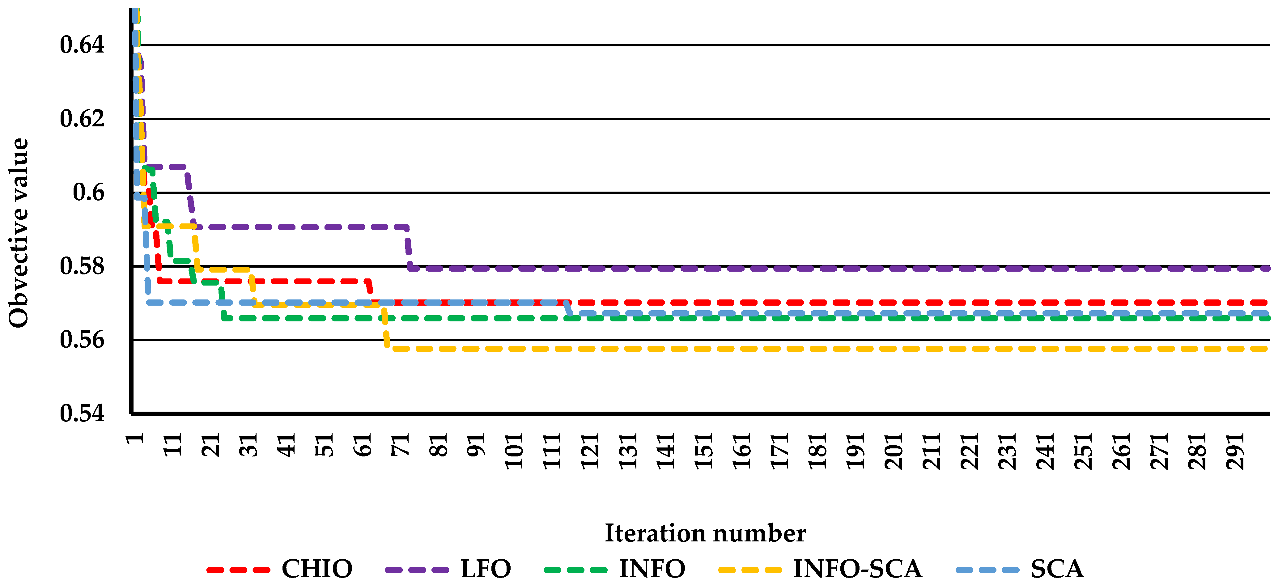
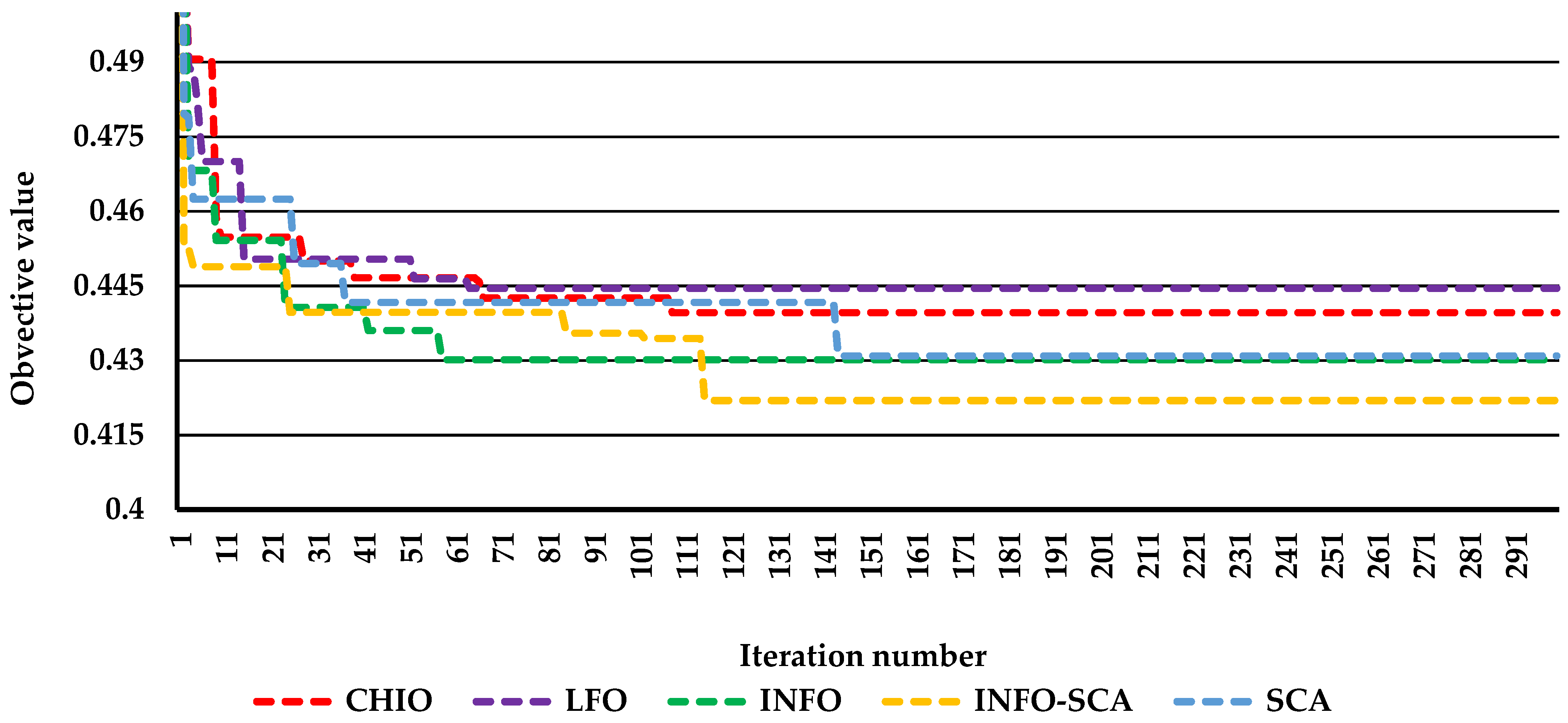
4.5. Testing the Performance of the INFO-SCA

To evaluate the performance of the hybrid of INFO and SCA, INFO-SCA was compared with INFO, SCA, the coronavirus herd immunity optimizer (CHIO) [54], and the Lévy flight distribution algorithm (LFO) [55]. The evaluation process was conducted in terms of the time consumed to carry out one run (T_run), and the best and worst values. It is worth mentioning that the population size was 30 for all algorithms, and the maximum number of iterations was 300. At the same time, the maximum number of runs was 30.

Table 6. Simulation results of the five algorithms for the EHVN.

Algorithm	Objective Value		Trun (s)
	Best	Worst
INFO-SCA	0.421957	0.445141	400.38
INFO	0.430142	0.45530	370.24
SCA	0.430912	0.45521	362.15
CHIO	0.439621	0.46301	453.32
LFO	0.444512	0.463221	443.05

and

Table 7. Simulation results of the five algorithms for the 24-bus system.

Algorithm	Objective Value		Trun (s)
	Best	Worst
INFO-SCA	0.557634	0.58053	805.35
INFO	0.565905	0.58432	781.02
SCA	0.567239	0.5902	770.54
CHIO	0.570144	0.5885	844.41
LFO	0.579398	0.5902	823.62

show the obtained results of all algorithms of the first scenario for the EHVN and the IEEE 24-bus system. The results demonstrated the efficiency of INFO-SCA in solving the problem. INFO-SCA mastered the best solutions in acceptable computational time. Figure 19 and Figure 20 illustrate the convergence curves of the five techniques for both systems. For EHVN, INFO-SCA needed about 115 iterations to reach the best solutions, whilst INFO, SCA, CHIO, and LFO converged in about 58, 141, 108, and 64 iterations, respectively. On the other hand, INFO-SCA needed about 68 iterations to reach the best solutions for the 24-bus system, while INFO, SCA, CHIO, and LFO needed about 25, 116, 64, and 73 iterations, respectively.

It is shown that the parallel operation mechanism of SCA and INFO improved the exploration and exploiting phases of both algorithms. Unlike individual algorithms, the best solution in each iteration obtained by one of the optimizers helped the other to explore a better search area in the next iterations [56]. More exploration and exploitation areas were investigated because of the unique updating scheme featured in each optimizer. The combined scheme was able to avoid stagnation at the local optimums. Further, reaching the global optimum for large-scale problems can be achieved in a minimum number of runs.

5. Conclusions

In this paper, the HC planning model was suggested and examined to increase the use of RSESs and fulfill future load demands. Furthermore, a long-term load forecasting method based on ANFIS was integrated with the planning model to predict the future increase in electrical loads. The PSP problem was formulated as an optimization problem to increase the HC for networks as a priority. The objective function aimed to determine the optimal projects for the generation and transmission expansion and decide the location and size for ESSs and FCLs required to achieve the problem constraints and avoid load shedding. In addition to the operational constraints, the reliability constraints such as N-1 security and short-circuited current constraints were considered. The problem was complex and formulated as a non-linear large-scale optimization problem. To solve it, the hybrid INFO-SCA was applied.

For the two investigated test systems, the suggested model succeeded to exploit all RSESs’ available power over planning scenarios. The HC in EHVN reached 100% over some scenarios, while it was 78.52% of the IEEE 24-bus system. The LCOE was applied in this work to consider the economic aspect of the installed projects. It was about 0.006 million USD/MWh for EHVN, while it was about 0.0223 million USD/MWh for the 24-bus system. Also, it was shown for both test systems that hybrid INFO-SCA was superior in reaching high-quality solutions compared to SCA and INFO. However, SCA had the fastest convergence speed. The results proved the efficiency of ANFIS in forecasting the annual load growth compared to some methods from the literature.

References

1. International Energy Outlook 2021-U.S. Energy Information Administration (EIA). Available online: https://www.eia.gov/outlooks/ieo/ (accessed on 31 January 2022).
2. Sinsel, S.R.; Riemke, R.L.; Hoffmann, V.H. Challenges and solution technologies for the integration of variable renewable energy sources—A review. Renew. Energy 2020, 145, 2271–2285. [Google Scholar] [CrossRef]
3. Refaat, M.M.; Abdel Aleem, S.H.E.; Atia, Y.; Ali, Z.M.; El-Shahat, A.; Sayed, M.M. A mathematical approach to simultaneously plan generation and transmission expansion based on fault current limiters and reliability constraints. Mathematics 2021, 9, 2771. [Google Scholar] [CrossRef]
4. Ismael, S.M.; Abdel Aleem, S.H.E.; Abdelaziz, A.Y.; Zobaa, A.F. State-of-the-art of hosting capacity in modern power systems with distributed generation. Renew. Energy 2019, 130, 1002–1020. [Google Scholar] [CrossRef]
5. Rabiee, A.; Mohseni-bonab, S.M. Maximizing hosting capacity of renewable energy sources in distribution networks: A multi-objective and scenario-based approach. Energy 2017, 120, 417–430. [Google Scholar] [CrossRef]
6. Santos, S.F.; Fitiwi, D.Z.; Shafie-Khah, M.; Bizuayehu, A.W.; Cabrita, C.M.P.; Catalão, J.P.S. New multi-stage and stochastic mathematical model for maximizing RES hosting capacity—Part I: Problem formulation. IEEE Trans. Sustain. Energy 2016, 8, 304–319. [Google Scholar] [CrossRef]
7. Santos, F.; Fitiwi, D.Z.; Member, S.; Shafie-khah, M.; Bizuayehu, A.W.; Cabrita, C.M.P.; Catal, P.S. New Multi-Stage and Stochastic Mathematical Model for Maximizing RES Hosting Capacity—Part II: Numerical Results. IEEE Trans. Sustain. Energy 2017, 8, 320–330. [Google Scholar] [CrossRef]
8. Bletterie, B.; Le Baut, J.; Kadam, S.; Bolgaryn, R.; Abart, A. Hosting Capacity of LV Networks with Extended Voltage Band. In Proceedings of the Proceedings—2015 International Symposium on Smart Electric Distribution Systems and Technologies (EDST), Vienna, Austria, 8–11 September 2015; IEEE: Washington, DC, USA, 2015; pp. 531–536. [Google Scholar]
9. Etherden, N.; Bollen, M.H.J. Increasing the hosting capacity of distribution networks by curtailment of renewable energy resources. In Proceedings of the 2011 IEEE Trondheim PowerTech, Trondheim, Norway, 19–23 June 2011; IEEE: Washington, DC, USA, 2011; pp. 1–7. [Google Scholar]
10. Etherden, N.; Bollen, M.H.J. Dimensioning of energy storage for increased integration of wind power. IEEE Trans. Sustain. Energy 2013, 4, 546–553. [Google Scholar] [CrossRef]
11. Navarro-Espinosa, A.; Ochoa, L.F. Increasing the PV hosting capacity of Lv networks: OLTC-fitted transformers vs. reinforcements. In Proceedings of the 2015 IEEE Power and Energy Society Innovative Smart Grid Technologies Conference, ISGT 2015, Washington, DC, USA, 18–20 February 2015. [Google Scholar]
12. Sakar, S.; Balci, M.E.; Abdel, S.H.E.; Zobaa, A.F. Integration of large- scale PV plants in non-sinusoidal environments: Considerations on hosting capacity and harmonic distortion limits. Renew. Sustain. Energy Rev. 2018, 82, 176–186. [Google Scholar] [CrossRef] [Green Version]
13. Gacitua, L.; Gallegos, P.; Henriquez-Auba, R.; Lorca; Negrete-Pincetic, M.; Olivares, D.; Valenzuela, A.; Wenzel, G. A comprehensive review on expansion planning: Models and tools for energy policy analysis. Renew. Sustain. Energy Rev. 2018, 98, 346–360. [Google Scholar] [CrossRef]
14. Mahdavi, M.; Sabillon Antunez, C.; Ajalli, M.; Romero, R. Transmission Expansion Planning: Literature Review and Classification. IEEE Syst. J. 2019, 13, 3129–3140. [Google Scholar] [CrossRef]
15. Gomes, P.V.; Saraiva, J.T. State-of-the-art of transmission expansion planning: A survey from restructuring to renewable and distributed electricity markets. Int. J. Electr. Power Energy Syst. 2019, 111, 411–424. [Google Scholar] [CrossRef]
16. Refaat, M.M.; Aleem, S.H.E.A.; Atia, Y.; Ali, Z.M.; Sayed, M.M. AC and DC Transmission Line Expansion Planning Using Coronavirus Herd Immunity Optimizer. In Proceedings of the 2021 22nd International Middle East Power Systems Conference (MEPCON), Assiut, Egypt, 14–16 December 2021; pp. 313–318. [Google Scholar]
17. Refaat, M.M.; Aleem, S.H.E.A.; Atia, Y.; Ali, Z.M.; Sayed, M.M. Multi-stage dynamic transmission network expansion planning using lshade-spacma. Appl. Sci. 2021, 11, 2155. [Google Scholar] [CrossRef]
18. Alhamrouni, I.; Khairuddin, A.; Ferdavani, A.K.; Salem, M. Transmission expansion planning using AC-based differential evolution algorithm. IET Gener. Transm. Distrib. 2014, 8, 1637–1644. [Google Scholar] [CrossRef]
19. Luburić, Z.; Pandžić, H.; Carrión, M. Transmission expansion planning model considering battery energy storage, TCSC and LINEs using AC OpF. IEEE Access 2020, 8, 203429–203439. [Google Scholar] [CrossRef]
20. Hamidpour, H.; Aghaei, J.; Pirouzi, S.; Dehghan, S.; Niknam, T. Flexible, reliable, and renewable power system resource expansion planning considering energy storage systems and demand response programs. IET Renew. Power Gener. 2019, 13, 1862–1872. [Google Scholar] [CrossRef]
21. Esmaili, M.; Ghamsari-Yazdel, M.; Amjady, N.; Chung, C.Y.; Conejo, A.J. Transmission Expansion Planning including TCSCs and SFCLs: A MINLP Approach. IEEE Trans. Power Syst. 2020, 35, 4396–4407. [Google Scholar] [CrossRef]
22. Gan, W.; Ai, X.; Fang, J.; Yan, M.; Yao, W.; Zuo, W.; Wen, J. Security constrained co-planning of transmission expansion and energy storage. Appl. Energy 2019, 239, 383–394. [Google Scholar] [CrossRef]
23. Romero, R.; Rocha, C.; Mantovani, M.; Mantovani, J.R.S. Analysis of heuristic algorithms for the transportation model in static and multi-stage planning in network expansion systems. IEE Proc.-Gener. Transm. Distrib. 2003, 150, 521–526. [Google Scholar] [CrossRef]
24. Silva Sousa, A.; Asada, E.N. Combined heuristic with fuzzy system to transmission system expansion planning. Electr. Power Syst. Res. 2011, 81, 123–128. [Google Scholar] [CrossRef]
25. Shayeghi, H.; Mahdavi, M.; Bagheri, A. Discrete PSO algorithm based optimization of transmission lines loading in TNEP problem. Energy Convers. Manag. 2010, 51, 112–121. [Google Scholar] [CrossRef]
26. Shayeghi, H.; Mahdavi, M.; Bagheri, A. An improved DPSO with mutation based on similarity algorithm for optimization of transmission lines loading. Energy Convers. Manag. 2010, 51, 2715–2723. [Google Scholar] [CrossRef]
27. Fathy, A.A.; Elbages, M.S.; El-Sehiemy, R.A.; Bendary, F.M. Static transmission expansion planning for realistic networks in Egypt. Electr. Power Syst. Res. 2017, 151, 404–418. [Google Scholar] [CrossRef]
28. Leite Da Silva, A.M.; Rezende, L.S.; Da Fonseca Manso, L.A.; De Resende, L.C. Reliability worth applied to transmission expansion planning based on ant colony system. Int. J. Electr. Power Energy Syst. 2010, 32, 1077–1084. [Google Scholar] [CrossRef]
29. Eslami, M.; Neshat, M.; Khalid, S.A. A Novel Hybrid Sine Cosine Algorithm and Pattern Search for Optimal Coordination of Power System Damping Controllers. Sustainability 2022, 14, 541. [Google Scholar] [CrossRef]
30. Neshat, M.; Mirjalili, S.; Sergiienko, N.Y.; Esmaeilzadeh, S.; Amini, E.; Heydari, A.; Garcia, D.A. Layout optimisation of offshore wave energy converters using a novel multi-swarm cooperative algorithm with backtracking strategy: A case study from coasts of Australia. Energy 2022, 239, 122463. [Google Scholar] [CrossRef]
31. Chen, K.; Zhou, F.; Yin, L.; Wang, S.; Wang, Y.; Wan, F. A hybrid particle swarm optimizer with sine cosine acceleration coefficients. Inf. Sci. Ny. 2018, 422, 218–241. [Google Scholar] [CrossRef]
32. Najjar, M.; Falaghi, H. Wind-integrated simultaneous generation and transmission expansion planning considering short-circuit level constraint. IET Gener. Transm. Distrib. 2019, 13, 2808–2818. [Google Scholar] [CrossRef]
33. Moradi-Sepahvand, M.; Amraee, T. Hybrid AC/DC Transmission Expansion Planning Considering HVAC to HVDC Conversion under Renewable Penetration. IEEE Trans. Power Syst. 2021, 36, 579–591. [Google Scholar] [CrossRef]
34. Naderi, E.; Pourakbari-Kasmaei, M.; Lehtonen, M. Transmission expansion planning integrated with wind farms: A review, comparative study, and a novel profound search approach. Int. J. Electr. Power Energy Syst. 2020, 115, 105460. [Google Scholar] [CrossRef]
35. Mazaheri, H.; Ranjbar, H.; Saber, H.; Moeini-Aghtaie, M. Expansion planning of transmission networks. In Uncertainties in Modern Power Systems; Academic Press: Cambridge, MA, USA, 2021; pp. 35–56. [Google Scholar]
36. Ramirez, J.M.; Hernandez-Tolentino, A.; Marmolejo-Saucedo, J.A. A stochastic robust approach to deal with the generation and transmission expansion planning problem embedding renewable sources. In Uncertainties in Modern Power Systems; Academic Press: Cambridge, MA, USA, 2021; pp. 57–91. [Google Scholar]
37. Zhou, Y.; Zhai, Q.; Yuan, W.; Wu, J. Capacity expansion planning for wind power and energy storage considering hourly robust transmission constrained unit commitment. Appl. Energy 2021, 302, 117570. [Google Scholar] [CrossRef]
38. Abushamah, H.A.S.; Haghifam, M.R.; Bolandi, T.G. A novel approach for distributed generation expansion planning considering its added value compared with centralized generation expansion. Sustain. Energy Grids Netw. 2021, 25, 100417. [Google Scholar] [CrossRef]
39. Zhang, H.; Cheng, H.; Liu, L.; Zhang, S.; Zhou, Q.; Jiang, L. Coordination of generation, transmission and reactive power sources expansion planning with high penetration of wind power. Int. J. Electr. Power Energy Syst. 2019, 108, 191–203. [Google Scholar] [CrossRef]
40. Mortaz, E.; Valenzuela, J. Evaluating the impact of renewable generation on transmission expansion planning. Electr. Power Syst. Res. 2019, 169, 35–44. [Google Scholar] [CrossRef]
41. Zhuo, Z.; Du, E.; Zhang, N.; Kang, C.; Xia, Q.; Wang, Z. Incorporating Massive Scenarios in Transmission Expansion Planning with High Renewable Energy Penetration. IEEE Trans. Power Syst. 2020, 35, 1061–1074. [Google Scholar] [CrossRef]
42. Akhavizadegan, F.; Wang, L.; McCalley, J. Scenario selection for iterative stochastic transmission expansion planning. Energies 2020, 13, 1203. [Google Scholar] [CrossRef] [Green Version]
43. Ahmadianfar, I.; Asghar Heidari, A.; Noshadian, S.; Chen, H.; Gandomi, A.H. INFO: An Efficient Optimization Algorithm based on Weighted Mean of Vectors. Expert Syst. Appl. 2022, 195, 116516. [Google Scholar] [CrossRef]
44. Mirjalili, S. SCA: A Sine Cosine Algorithm for solving optimization problems. Knowl.-Based Syst. 2016, 96, 120–133. [Google Scholar] [CrossRef]
45. Biswas, P.P.; Suganthan, P.N.; Mallipeddi, R.; Amaratunga, G.A.J. Optimal reactive power dispatch with uncertainties in load demand and renewable energy sources adopting scenario-based approach. Appl. Soft Comput. J. 2019, 75, 616–632. [Google Scholar] [CrossRef]
46. Kamdar, I.; Ali, S.; Taweekun, J.; Ali, H.M. Wind Farm Site Selection Using WAsP Tool for Application in the Tropical Region. Sustainability 2021, 13, 13718. [Google Scholar] [CrossRef]
47. Mostafa, M.H.; Abdel Aleem, S.H.E.; Ali, S.G.; Ali, Z.M.; Abdelaziz, A.Y. Techno-economic assessment of energy storage systems using annualized life cycle cost of storage (LCCOS) and levelized cost of energy (LCOE) metrics. J. Energy Storage 2020, 29, 101345. [Google Scholar] [CrossRef]
48. Akdemir, B.; Çetinkaya, N. Long-term load forecasting based on adaptive neural fuzzy inference system using real energy data. Energy Procedia 2012, 14, 794–799. [Google Scholar] [CrossRef] [Green Version]
49. Şahin, M.; Erol, R. A Comparative Study of Neural Networks and ANFIS for Forecasting Attendance Rate of Soccer Games. Math. Comput. Appl. 2017, 22, 43. [Google Scholar] [CrossRef] [Green Version]
50. Renewables.ninja. Available online: https://www.renewables.ninja/ (accessed on 31 January 2022).
51. Egyptian Electricity Holding Company Annual Reports. Available online: http://www.moee.gov.eg/english_new/report.aspx (accessed on 31 January 2022).
52. Zhang, H.; Heydt, G.T.; Vittal, V.; Mittelmann, H.D. Transmission expansion planning using an AC model: Formulations and possible relaxations. In Proceedings of the 2012 IEEE Power and Energy Society General Meeting, San Diego, CA, USA, 22–26 July 2012; IEEE: Washington, DC, USA, 2012; pp. 1–8. [Google Scholar]
53. Saboori, H.; Hemmati, R. Considering carbon capture and storage in electricity generation expansion planning. IEEE Trans. Sustain. Energy 2016, 7, 1371–1378. [Google Scholar] [CrossRef]
54. Al-Betar, M.A.; Alyasseri, Z.A.A.; Awadallah, M.A.; Abu Doush, I. Coronavirus Herd Immunity Optimizer (CHIO); Springer: London, UK, 2021; Volume 33, ISBN 0123456789. [Google Scholar]
55. Houssein, E.H.; Saad, M.R.; Hashim, F.A.; Shaban, H.; Hassaballah, M. Lévy flight distribution: A new metaheuristic algorithm for solving engineering optimization problems. Eng. Appl. Artif. Intell. 2020, 94, 103731. [Google Scholar] [CrossRef]
56. Zobaa, A.F.; Aleem, S.H.E.A.; Abdelaziz, A.Y. Classical and Recent Aspects of Power System Optimization; Academic Press: Cambridge, MA, USA; Elsevier: Amsterdam, The Netherlands, 2018; ISBN 9780128124413. [Google Scholar]
Figure 1. Hosting capacity problems and enhancement techniques.
Sustainability 14 02998 g001
Figure 2. The applied forecasting and planning scheme.
Sustainability 14 02998 g002
Figure 3. Initial configuration of the EHVN, adopted from [27].
Sustainability 14 02998 g003
Figure 4. Selected testing scenarios.
Sustainability 14 02998 g004
Figure 5. Initial configuration of the IEEE 24- bus system, adopted from [52].
Sustainability 14 02998 g005
Figure 6. Load forecasting using ANFIS and three mathematical methods (linear-, parabola-, and exponential- based models).
Sustainability 14 02998 g006
Figure 7. Load growth until the year 2040 using ANFIS.
Sustainability 14 02998 g007
Figure 8. Final configuration of EHVN.
Sustainability 14 02998 g008
Figure 9. Percentage of HC over the two representative days for the EHVN.
Sustainability 14 02998 g009
Figure 10. Charging and discharging powers of ESSs at each scenario for the EHVN.
Sustainability 14 02998 g010
Figure 11. SOC of ESSs over the two representative days for the EHVN.
Sustainability 14 02998 g011
Figure 12. Maximum of short circuit current at each scenario for the EHVN.
Sustainability 14 02998 g012
Figure 13. Impact of ω g and ω E S S on expansion projects.
Sustainability 14 02998 g013
Figure 14. Final configuration of the 24-bus system.
Sustainability 14 02998 g014
Figure 15. Maximum of short circuit current at each scenario for the 24-bus system.
Sustainability 14 02998 g015
Figure 16. Percentage of HC over the two representative days for the 24-bus system.
Sustainability 14 02998 g016
Figure 17. Charging and discharging powers of ESSs over the first 24 h for the 24-bus system.
Sustainability 14 02998 g017
Figure 18. SOC of ESSs over the two representative days for the 24-bus system.
Sustainability 14 02998 g018
Figure 19. Convergence curves of the five algorithms for the EHVN.
Sustainability 14 02998 g019
Figure 20. Convergence curves of the five algorithms for the 24-bus system.
Sustainability 14 02998 g020