A New Container Throughput Forecasting Paradigm under COVID-19

Abstract

COVID-19 has imposed tremendously complex impacts on the container throughput of ports, which poses big challenges for traditional forecasting methods. This paper proposes a novel decomposition–ensemble forecasting method to forecast container throughput under the impact of major events. Combining this with change-point analysis and empirical mode decomposition (EMD), this paper uses the decomposition–ensemble methodology to build a throughput forecasting model. Firstly, EMD is used to decompose the sample data of port container throughput into multiple components. Secondly, fluctuation scale analysis is carried out to accurately capture the characteristics of the components. Subsequently, we tailor the forecasting model for every component based on the mode analysis. Finally, the forecasting results of all the components are combined into one aggregated output. To validate the proposed method, we apply it to a forecast of the container throughput of Shanghai port. The results show that the proposed forecasting model significantly outperforms its rivals, including EMD-SVR, SVR, and ARIMA.

1. Introduction

As an essential node for the realization of international trade, ports are not only the core infrastructure for building a global transportation system, but are also an important part of building an international supply chain [1]. The operation of the port transportation industry is a “barometer” of national macro-economy. The fluctuation of container throughput can directly reflect the prosperity and development of word trade. The sudden outbreak and spread of COVID-19 has had a great impact on the safe operation and management of China’s ports in the short term [2].

The World Health Organization (WHO) declared the outbreak of COVID-19 to be a public health emergency of international concern on 31 January 2020, and defined COVID-19 as a pandemic on 11 March 2020 [3]. In order to control the spread of the epidemic, governments around the world have taken different levels of preventive and control measures, which, while interrupting the spread of the virus, have also negatively impacted maritime trade. Measures such as restrictions on ship activity and work stoppages can lead to a decline in transportation and hinder the development of the world economy [4,5]. The scale and duration of the impact of COVID-19 will cause fluctuations and oscillations in port container throughput.

The time series of port container throughput is superimposed by linear or nonlinear data, and is usually affected by accidental events. The reasonable decision of port management for the influence of major events relies on the reliability and superiority of forecasting. The accurate forecasting of the container throughput is central to the planning of the government transportation departments at the micro and macro levels; it also plays an important role in the investment planning and stable operations of the port [6].

However, the container throughput data contains a variety of complex superimposed components. The traditional forecasting techniques cannot effectively capture the impact of major events on the forecast results, and it is difficult to obtain forecast results that can be used to guide practice. It is necessary to establish a port container throughput forecasting method with high extensibility and that is suitable for the common scenarios of major events. To remedy the above shortcomings, this paper proposes a decomposition–ensemble forecasting method (EMD-Event Analysis-ARIMA-SVR (EEAS)) which applies the event analysis into container throughput forecasting. Firstly, the EMD is used to decompose the original observed data into a finite number of Intrinsic Mode Functions (IMFs). Then, the data characteristics of different IMFs are analyzed by means of a smoothness test, model fluctuation scale analysis, structural breakpoint test, etc. Subsequently, the components are predicted by using ARIMA or SVR according to the data characteristics and the results of significant event determination. Finally, the final forecasting results are obtained by ADD. The results show that the proposed model can effectively capture the degree of impact of the new crown epidemic on container throughput, and the forecasting accuracy is higher than that of EMD-SVR, SVR, and ARIMA.

The main contributions of this paper are as follows: (1) this paper proposes a novel decomposition–ensemble forecasting framework for port container throughput in the context of major events. The proposed model is not only tailored to container throughput forecasting under COVID-19, but also can be applied for impact analysis and forecasting in the context of major events, e.g., hurricanes and earthquakes. (2) This paper expands the application of EMD-based event analysis methods to port container throughput forecasting. Event analysis is introduced into the decomposition–ensemble forecasting model, and significant accuracy is achieved in the empirical forecasting analysis. (3) This paper is the first study to forecast the container throughput under COVID-19, and the proposed model is a powerful tool for port operation and investment planning.

This paper will introduce the impact of the epidemic on port container throughput and the application of throughput forecasting model in Section 2. Here, the application research of the decomposition–ensemble model is also thoroughly discussed. The research model and related theoretical ideas are described in detail in Section 3. Experimental verification is carried out with data to prove the reliability of the model in Section 4. Section 5 presents the conclusions and suggests some directions for future research.

2. Literature Review

This paper proposes a decomposition–ensemble forecasting method which applies an event analysis to port container throughput forecasting in the context of an epidemic. Therefore, the paper is related to the research topics on forecasting models, decomposition methods in forecasting, and forecasting considering COVID-19.

2.1. Forecasting Model

Predictive techniques can generally be divided into three main categories: econometric models, artificial intelligence models (AI), and hybrid algorithms.

In the field of container throughput forecasting, some traditional economic models have been frequently used, such as the autoregressive integrated moving average (ARIMA) model [7], the seasonal autoregressive integrated moving average (SARIMA) model [8,9], the exponential smoothing model [10], the error correction model (ECM) [11], the auto-regressive conditional heteroscedasticity (ARCH) model [12], the multiple regression model [13], the vector autoregressive (VAR) model [14], and the grey forecasting model [15,16]. However, these econometric models are unable to capture the nonlinear part of the original data. These econometric models have poor forecasting performance, particularly with regard to some nonlinear time series data.

Therefore, artificial intelligence (AI) models are used to describe nonlinear characteristics in the time series of container throughput. These AI models include the grey neural network [17,18], the discrete particle swarm optimization [19,20], the back-propagation neural network (BPNN) model [21], fuzzy neural networks [22], etc. In recent years, artificial intelligence technology has been constantly innovated and developed. Yu et al. [23] mentioned that, in the application of artificial intelligence technology, SVR (support vector regression algorithm), LSSVR (least squares support vector regression algorithm), and ANN (artificial neural network algorithm) are considered as the main applied artificial intelligence forecasting models. These three models can predict linear stationary and nonlinear stationary data with high precision, which are superior to econometric models in terms of forecasting performance (e.g., ARIMA). However, artificial intelligence models also have drawbacks such as the potential local optimum, the sensitivity of parameter selection [24], and complex computational operations.

Substantial hybrid approaches have been developed for better forecasting performance. Huang et al. [25] combined projection pursuit regression (PPR) with a genetic programming (GP) algorithm and proposed a hybrid method to forecast the container throughput of Qingdao Port. Based on the hybrid theory, Yu et al. [26] proposed a “decomposition and ensemble” or “divide and conquer” approach.

2.2. Decomposition Methods in Forecasting

By decomposition and ensemble, the proposed method can effectively improve the forecasting accuracy [23]. Xie et al. [27] proposed a hybrid forecasting method based on a combination of least squares supported vector regression (LSSVR) and a preprocessing method that includes SARIMA, seasonal decomposition (SD), and classical decomposition (CD). Yu et al. [28] proposed a sparse representation (SR) as a decomposition tool for the integrated forecasting of complex time series, greatly improving the forecasting accuracy of crude oil prices. Jianwei et al. [29] used variational mode decomposition (VMD) to decompose and forecast oil prices. Yu et al. [30] applied EMD-based neural network ensemble learning paradigms to forecast the world crude oil spot price. EMD is a common data decomposition tool proposed by Huang et al. [31]. This method decomposed nonlinear and non-stationary time series into several Intrinsic Mode Functions (IMFs). EMD has been widely used in many fields. EMD also provides a multi-scale framework to analyze the impact of extreme events, which has been successfully applied to crude oil price analysis, among others [32,33]. In order to grasp the impact of the epidemic event on each model feature of the port, the iterative cumulative sum of squares (ISCC) algorithm and Chow test mentioned by Inclán and Tiao [34] can be combined to conduct the structural change-point test for each feature model. The EMD decomposition tool is considered as a powerful data decomposition tool with a wide range of applications.

Most of the current forecasting studies employing various decomposition algorithms directly use components of the original data for forecasting without applying event analysis. This paper proposes a hybrid decomposition–ensemble forecasting model applying the event analysis to the container throughput forecasting tasks, which provides a powerful tool for forecasting tasks considering the impact of major events, e.g., COVID-19. Moreover, we extend the application of EMD-based event analysis by applying it to port container throughput forecasting.

2.3. Forecasting Considering COVID-19

Many scholars analyze the epidemic to improve the forecasting accuracy and study the impact of the epidemic on the fluctuation of the forecasting. Wu et al. [35] proposed a novel oil price, production, and consumption forecasting methodology. They input the text features of oil news headlines in the context of COVID-19 into some common forecasting models, such as BPNN, SVM, etc. Wu et al. [36] forecast crude oil prices by using convolutional neural network (CNN) and variational mode decomposition (VMD) to extract and process text features in online news. Weng et al. [37] proposed a modeling framework, the genetic algorithm regularization online extreme learning machine with forgetting factor (GA-RFOS-ELM), to estimate the effects of news during COVID-19 on the volatility of crude oil futures. Stifanic et al. [38] integrated the stationary wavelet transform (SWT) and bidirectional long short-term memory (BDLSTM) networks to predict commodity and stock price movement during COVID-19. Koyuncu et al. [39] forecast the container throughput index with the time series. They examined the relationship between the short-term estimate of the container throughput index and COVID-19.

A majority of current studies forecast crude oil prices, commodity prices, stock prices, container throughput index, etc., considering COVID-19. This paper is the first to address the container throughput under COVID-19.

Different from the existing studies, to the best of our knowledge, this is the first study to propose a hybrid decomposition–ensemble forecasting model integrating event analysis into the container throughput forecasting tasks, which provides a powerful tool for forecasting tasks considering the impact of major events, e.g., COVID-19. Furthermore, our paper applies EMD-based event analysis into port container throughput forecasting to expand the application of event analysis. We compare the existing studies with our study in

Table 1. Comparisons between pertinent studies and our study.

Literature	Model	Mixed Model	AI Model	The Impact of Major Events	Decomposition–Ensemble Model
Rashed et al. [7]	ARIMA	×	×	×	×
Farhan et al. [8]	SARIMA	×	×	×	×
Ruiz et al. [9]	SARIMA-ANN	√	√	×	×
Schulze et al. [10]	SARIMA and Holt–Winters	×	×	×	×
Fung et al. [11]	Error-correction model	×	×	×	×
Munim et al. [12]	ARIMA-ARCH	√	×	×	×
Veenstra et al. [13]	Vector autoregressive model	×	×	×	×
Gao et al. [14]	Structural change VAR model	×	×	×	×
Peng et al. [15]	Grey model	×	×	×	×
Guo et al. [16]	Grey model	×	×	×	×
Ding et al. [17]	BP Neural Network	×	√	×	×
He et al. [18]	GM(1,1)-BPNN	√	√	×	×
Jing et al. [19]	MARS-RSVR	√	√	×	×
Xiao et al. [20]	TF-DPSO	√	√	×	×
Liu et al. [21]	BPNN	×	√	×	×
Milenkovic et al. [22]	FNN	×	√	×	×
Yu et al. [23]	EEMD-DCD-ANN, EEMD-DCD-LSSVR	√	√	×	√
Tang et al. [24]	EEMD-LSSVR	√	√	×	√
Hang et al. [25]	PPR-GP	√	√	×	×
Yu et al. [26]	EMD-LSTM-ELM	√	√	×	√
Xie et al. [27]	SARIMA-LSSVR, SD-LSSVR, and CD–LSSVR	√	√	×	√
Yu et al. [28]	SR-FNN-ADD	√	√	×	√
Jianwei et al. [29]	VMD-ICA-ARIMA	√	√	×	√
Yu et al. [30]	EMD-FNN-ALNN	√	√	×	√
Wu et al. [35]	CNN-BPNN/MLR/SVM/LSTM/RNN	√	√	√	×
Wu et al. [36]	CNN-VMD	√	√	√	×
Weng et al. [37]	GA-RFOS-ELM	√	√	√	×
Stifanic et al. [38]	BDLSTM + WT-ADA	√	√	√	√
Koyuncu et al. [39]	SARIMA and ETS	×	×	×	×
This paper	EMD-Event Analysis-ARIMA-SVR	√	√	√	√

.

3. Methodology Formulation

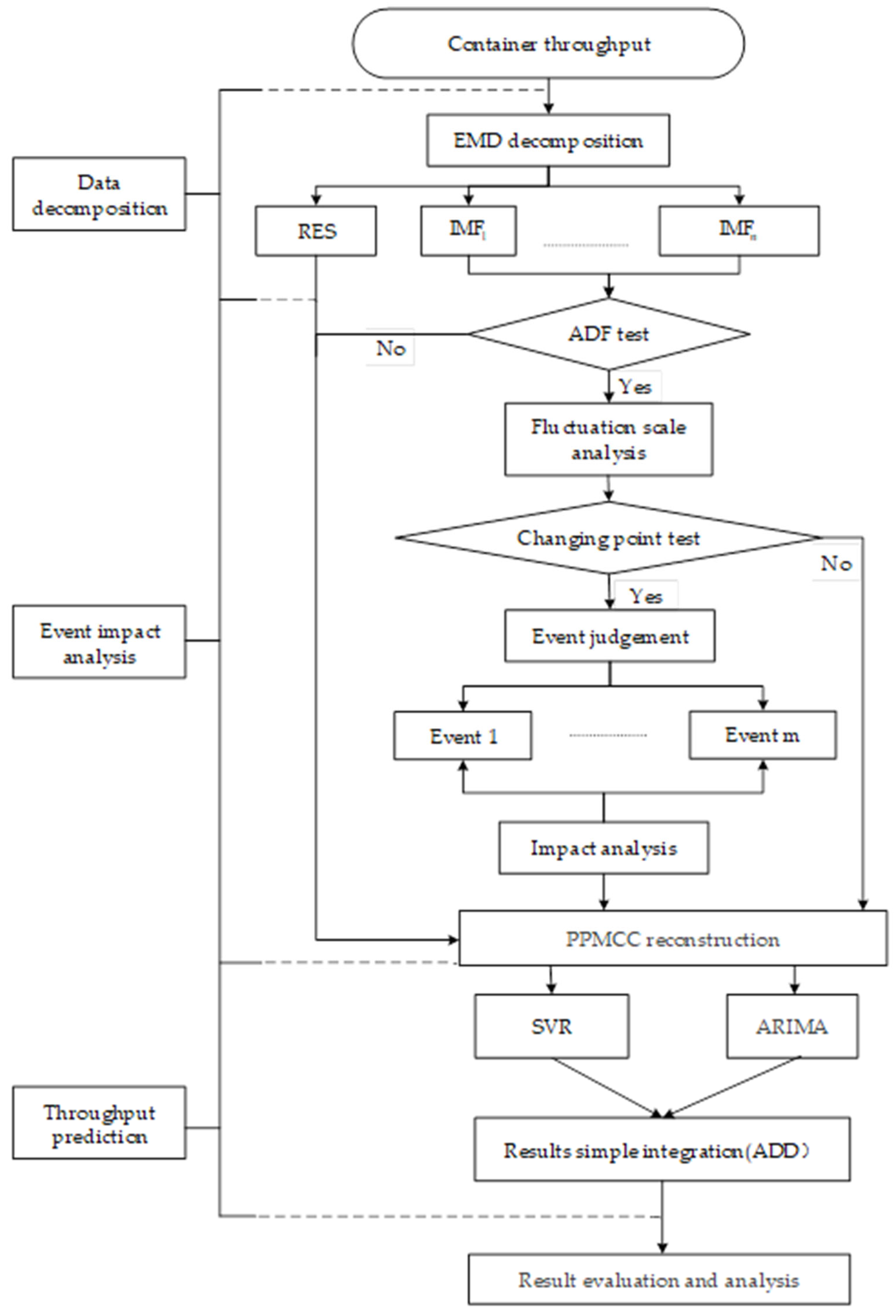
3.1. Framework of the Proposed Methodology

To explore the impact of COVID-19 on port container throughput and improve the forecasting accuracy, a decomposition–ensemble methodology is proposed based on event analysis. This method actually improves the existing decomposition–ensemble technology in the framework of “divide and conquer” [40]. By incorporating EMD and a forecasting model, the event analysis and forecasting are integrated into a dual-function hybrid model.

The framework of this study is composed of the following three main steps, described in Figure 1.

Step 1: Decomposition stage. The empirical mode decomposition (EMD) is used to decompose the port container throughput.

Step 2: Analysis stage. The first screening of the decomposed components is completed by stationarity test, and the second screening is completed by structural change-point test to screen out the volatile components in the non-smoothness components. Then, statistical analysis and fluctuation scale analysis are carried out for the volatile component to quantify the impact of the epidemic on the port throughput.

Step 3: Forecasting stage. The model is selected and optimized to predict each component. Then, the forecasting results of the corresponding component are combined into the aggregated output of port container throughput forecasting.

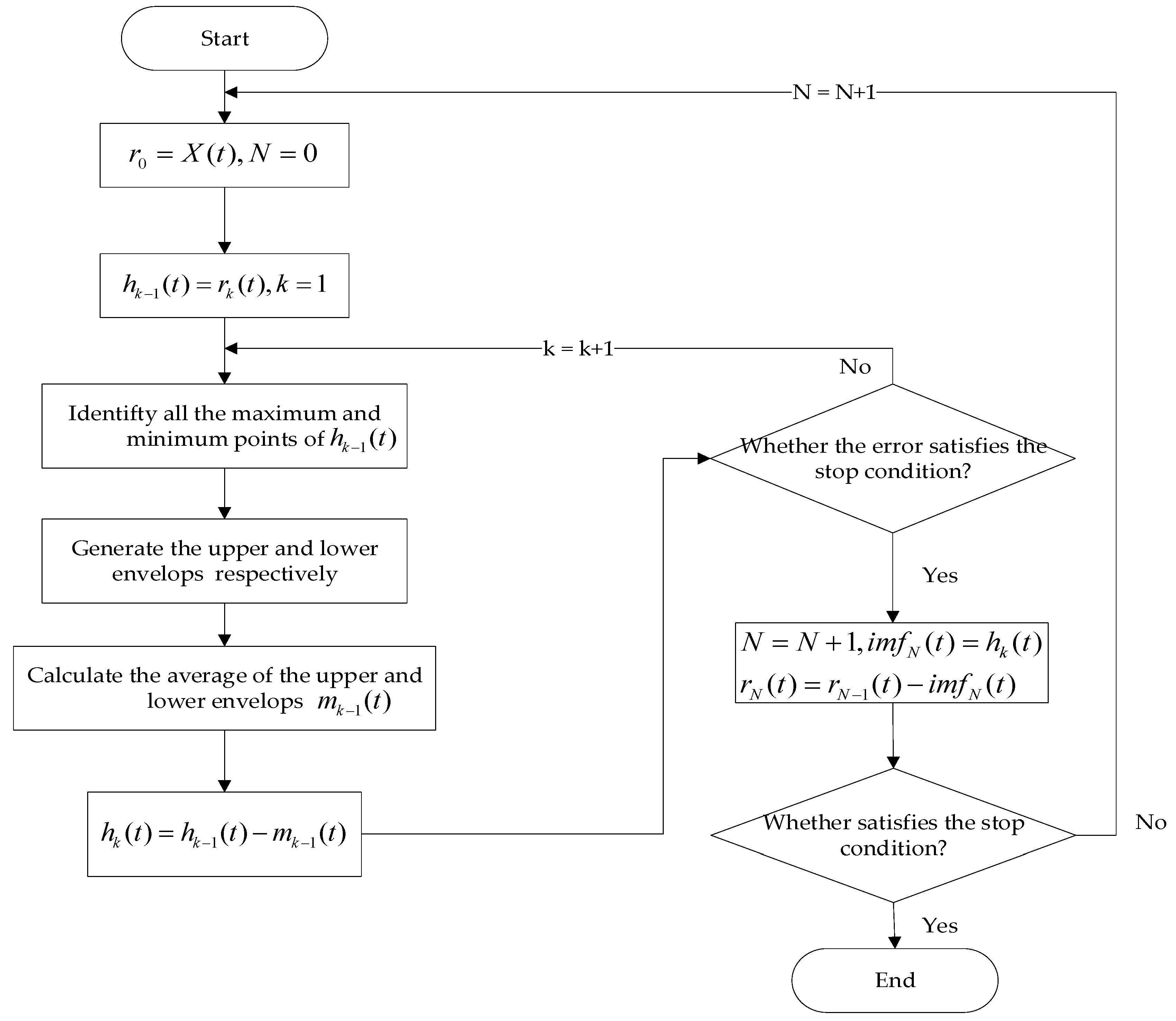
3.2. Data Decomposition

Empirical mode decomposition (EMD) is applied in this paper. EMD can effectively analyze the feature of the signal itself and truly extract the trend of the data series, so it is good at analyzing the correlation between components and their influence factors.

The EMD decomposition flow is presented in Figure 2. The original time series data can be expressed as follows [31]:

$$X_t={\sum }_{i=1}^{N}im{f}_i\left(t\right)+r_{N,t},$$

(1)

where N is the number of IMFs, $r_{N,t}$ is the residual component, and $im{f}_i\left(t\right) \left(i=1,2,...n\right)$ is the ith IMF at the time of $t$. IMF components with different frequencies are different, and they vary with $X_t$.

3.3. Mode Feature Analysis

In this part, we will conduct the structural change-point test analysis (change-point test). ICSS, proposed by Inclán and Tiao [34], is a well-established method for structural change-point testing. For the shortcomings of ICSS, a Chow test can be used for the change-point test. Finally, the results of the structural change-point test will be combined with an epidemic to conduct impact analysis. This section consists of the following steps: the stationary data components are screened out through a stationarity test; in the test, the ICSS algorithm and Chow test method are used to carry out a volatility test to explore how the epidemic affects the components.

3.3.1. Stationarity Test

A time series can be called stationary if there is no systematic change in the mean (no trend) or the variance, and if the periodic change is strictly eliminated. At present, the most popular stationarity test of time series data is the Augmented Dickey–Fuller (ADF) test. The test judges whether there is any unit root in the process of data generation. If there is no unit root, the time series data can be regarded to be stationary, and vice versa.

3.3.2. Fluctuation Scale Analysis

To obtain the characteristics of price fluctuations in different time scales, the IMFs of the estimation window and event window are statistically analyzed, respectively. We use three measures as follows: the fluctuation period, correlation coefficient, and variance proportion of IMF.

The volatility period is defined as the total number of points divided by the number of peaks in each IMF, and it indicates the vibration magnitude (influence period) of the IMF. $IM{F}_i$ is the $i\mathrm{th}\mathrm{IMF}.$A correlation coefficient is used to measure the relationship between a single component and the original time series. The variance proportion is measured as the ratio of IMF volatility to overall throughput volatility. Among them, the variance proportion is expressed as follows:

$$A_i=\frac{{\delta }_i}{\delta }$$

(2)

where ${\delta }_i$ is the variance of $IM{F}_i$, and $\delta$ is the sum of the variances of the components series.

In this paper, the phase variance percentage correlation coefficient will be used to screen out the components that can show the characteristics of the data, that is, the mode and the fluctuation rule.

3.3.3. Fluctuation Scale Analysis

A breakpoint test can be used to verify whether the sequence data has structural changes due to some extreme events. In this part, the ICSS algorithm and Chow test are applied to obtain structural changes.

In this paper, the ICSS algorithm is performed to find the suspect points (structural break points) of the screened IMF. The change point is verified by a Chow test, and the test divides the time series data into two parts according to the supposed change-point time. Finally, the F test, as shown in Equation (3), is used to check whether the parameters obtained from the previous part of the data are equal to those obtained from the latter part of the data, judging, thus, whether the structure has changed [34].

$$F=\frac{\frac{SSE-SS{E}_1-SS{E}_2}{m+1}}{\frac{SS{E}_1+SS{E}_2}{N_1+N_2-2m-2}}~F\left(m+1,N_1+N_2-2m-2\right),$$

(3)

where $m$ is the number of the explanatory variables,$N_1$ and $N_2$ are observations in the data subsets before and after the breakpoint$k$, and $SSE$ is the sum of residual squares in the modeling of the whole time series data with a degree of freedom of $N_1+N_2-m-1$. $SS{E}_1$ and $SS{E}_2$ are the sum of residual squares in the data subsets before and after the breakpoint $\mathrm{k}$, and their degrees of freedom are $N_1-m-1$ and $N_2-m-1$, respectively. Given the significance level $\mathsf{\alpha }$, if $F>F\left(m+1,N_1+N_2-2m-2\right)$, or $F<F\left(1-\alpha ,N_1+N_2-2m-2\right)$, then it indicates that the regression model is structurally unstable, and this point is the structural change point of the time series.

After the change-point test, this paper segments the corresponding IMF series and calculates the relevant indexes for each series. The relevant indexes include general statistics (i.e., maximum, minimum, difference, median, mean, variance), distribution (i.e., skewness, kurtosis, and probability), and each segment is compared. Finally, we conduct the event analysis based on the previous fluctuation scale analysis.

3.4. Throughput Forecasting

3.4.1. Reconstruction Clustering

We process the original throughput sequence data by EMD, and we obtain a series of throughput component IMFs with frequencies ranging from high to low. Then, we use the Pearson product–moment correlation coefficient (PPMCC) to reconstruct and aggregate the modes, to reduce the number of modes, as follows [41]:

$$R=\frac{1}{n-1}{\sum }_{i=1}^n\left(\frac{X_i-\overline{X}}{S_x}\right)\left(\frac{Y_i-\overline{Y}}{S_Y}\right) ,$$

(4)

where $n$ is the number of observed data, $X_i$ represents the observed data value of mode, and $Y_i$ is the observed data value of $m\left(t\right).\overline{X}$ and $\overline{Y}$ are the mean values of the observed sequence data. $S_x$ and $S_Y$ are the standard deviations of the observed sequence data. $m\left(t\right)$ represents the local mean of the original throughput sequence.

$$m\left(t\right)=0.5\times \left(a+b\right),$$

(5)

where$a$ is the lower envelope sequence of the original signal, while $b$ is the upper envelope sequence of the original signal.

During screening, the intrinsic mode components that are smaller than the contribution rate threshold are discarded, and the intrinsic mode components larger than the contribution rate threshold are extracted for the reconstruction and aggregation of time series data. Finally, by data feature-driven reconstruction, each mode is further reconstructed and aggregated into some valuable components.

3.4.2. Forecasting Model

(1)

ARIMA model

The ARIMA model is based on stationary time series, so the stationarity of time series is an important prerequisite for modeling. The general form of $\mathrm{ARIMA}\left(\mathrm{P},\mathrm{Q},\mathrm{d}\right)$ model is described by [42]:

$$y_t=C+{\alpha }_1{y}_{t-1}+\cdots {\alpha }_p{y}_{t-p}+{\theta }_1{\mu }_{t-1}+\cdots \theta q{\mu }_{t-q}+{\mu }_t,$$

(6)

where $y_{t-i}$ refers to the stationary sequence value, and it is obtained by a stationary test and differential exchange of $IM{F}_i$ and residual $r_{N,t}$. $p$ is the number of auto-regressive terms, $\theta$ is the moving average model coefficient, $q$ is the number of moving average terms, indicating the lag number of forecasting errors, and C is a constant. $\alpha$ is the coefficient of the auto-regressive model. ${\mu }_t$ is the random error term which is independent identically distributed, and it is a white noise sequence. Equation (6) consists an auto-regressive process and a moving average process.

When $C=0$, the model becomes a centralized $\mathrm{ARMA}\left(\mathrm{p},\mathrm{q}\right)$ model and when $\mathrm{q}=0$, Equation (6) becomes a $\mathrm{p}$-order autoregressive model, which is recorded as $\mathrm{AR}\left(\mathrm{P}\right)$. When $\mathrm{p}=0$, Equation (6) is called a q-order moving average model, which is recorded as $\mathrm{MA}\left(\mathrm{q}\right)$. In this paper, the establishment of the $\mathrm{ARIMA}$ model is the selection of $\mathrm{p},\mathrm{q}$, and $\mathrm{d}$. Each IMF and residual$r_{N,t}$ correspond to an $\mathrm{ARIMA}$ model.

(2)

SVR model forecasting

Vapnik et al. [43] systematically expounded the statistical theory of classification and regression problems and the concept and classification of SVM. They proposed a support vector machine-learning method, including support vector regression (SVR) and support vector classification (SVC). Support vector machine is a classification algorithm. Since different models can be made according to different input data, it can be also applied in regression. SVR is one of the specific applications of statistical learning theory and it can be transformed into solving a quadratic programming problem.

The minimization of structural risk can enhance the generalization ability of classifier. The empirical risk and confidence range are minimized, so as to obtain good statistical laws when the statistical sample size is small. The support vector regression problem can be described as follows.

The training sample data set is $\left\{\left(x_i, y_i\right)|i=1,2,3\dots n\right\}$, and $x_i$∈R, $y_i$∈R are the input and output target values, respectively. Then, the optimal linear regression function can be constructed as follows:

$$f\left(x\right)={\omega }^T\phi \left(x\right)+b,$$

(7)

where $f\left(x\right)$ is the estimation result of $x$, $\phi \left(x\right)$ maps the input vector $x$ into a vector in the feature space, and the weight ${\omega }^T$and bias$b$ are obtained by minimizing the regularized risk function of $\mathrm{SVR}$. If the regression function$f\left(x\right),$satisfying the changing relationship of each pair of $\left(x_i,y_i\right)$, is estimated according to the samples—so that the difference between $f\left(x\right)$ and $y_i$ are very small—then $f\left(x\right)$ can be performed to predict the $y_i$ corresponding to any $x_i$. The SVR problem can be described as:

$$\begin{array}{c}min \frac{1}{2}{\omega }^T\omega +\gamma {\sum }_{i=1}^m\left(e_i+e_i^{\ast }\right),\\ s.t.\{\begin{array}{c}{y}_i-\omega ·\phi \left(x\right)-b\le \epsilon +e_i\\ \omega ·\phi \left(x\right)+b-y_i\le \epsilon +e_i^{\ast }\\ e_i,e_i^{\ast }\ge 0\end{array},\end{array}$$

(8)

where $e_i$,${e_i}^{\ast }$ are the slack variables, $\epsilon$ is the error, and $\gamma >0$ is the penalty parameter, which is the penalty degree of the sample point. This is a quadratic programming problem, which is usually not solved directly. Then, we introduce Lagrange multipliers $\alpha and \eta$ to transform the above constrained optimization problem into an unconstrained optimization problem. Thus, the problem becomes a dual problem to solve, which can be expressed as:

$$\begin{array}{cc}L\left(\omega ,b,e,\alpha \right)\hfill & =\frac{1}{2}{\omega }^T\omega +\gamma {\displaystyle {\displaystyle \sum }_{i=1}^m}\left(e_i+e_i^{\ast }\right)-{\displaystyle {\displaystyle \sum }_{i=1}^m}\left({\eta }_i{e}_i+{\eta }^{\ast }{e}_i^{\ast }\right)\hfill \\ \hfill & -{\displaystyle {\displaystyle \sum }_{i=1}^m}{\alpha }_i\left(\epsilon +e_i-y_i+\omega ·\phi \left(x\right)+b\right)-{\displaystyle {\displaystyle \sum }_{i=1}^m}{\alpha }_i^{\ast }\left(\epsilon +e_i^{\ast }+y_i-\omega ·\phi \left(x\right)-b\right).\hfill \end{array}$$

(9)

With the Karush–Kuhn–Tucker$\left(\mathrm{KKT}\right)$ optimization condition and the minimum optimization algorithm, the dual optimization problem is solved. After eliminating $e_i and \omega$, the kernel function $K{x}_i,x$ is defined, and after obtaining$\alpha$ and $b$, the optimal linear regression function expression of SVR can be obtained as follows:

$$f\left(x\right)={\sum }_{i=1}^n{\alpha }_i-{\alpha }_i^{\ast }K\left(x_i,x\right)+b,$$

(10)

where $K{x}_i,x$ is a kernel function and is and arbitrary symmetric function satisfying the $\mathrm{Mercer}$ condition, i.e., $K{x}_i,x_j=\phi {\left(x_i\right)}^T\phi \left(x_j\right)$. The four common kernel functions include a linear kernel, polynomial kernel, radial basis function $\left(\mathrm{RBF}\right),$and sigmoid kernel. The most commonly used kernel function is the RBF kernel, and the expression is as follows:

$$K\left(x_i,x\right)=exp\left(-\frac{\parallel x_i-x_j\parallel }{2{\sigma }^2}\right).$$

(11)

According to above process, SVR has only two parameters to select, $\gamma$ and ${\sigma }^2$, which can be obtained by solving the linear equations. In this paper, the optimal parameter combination ($\gamma ,{\sigma }^2)$ is obtained by the grid search algorithm. The grid search algorithm is an exhaustive attack method for specifying parameter values. Consequently, we add a new parameter forecasting lag $d$ for model optimization. The value of$d$ will be defined by the event analysis. In this paper, combined with the concept of data analysis, we optimize the combination of the $\left(d,\gamma , {\sigma }^2\right)$ parameters of the SVR model using the grid search method. Under the condition of $\gamma ϵ\left[{\gamma }_{min},{\gamma }_{max}\right]$ and $\sigma ϵ\left[{\sigma }_{min},{\sigma }_{man}\right]$, the minimum mean square error MSE is taken as the objective function $F$, which is solved by the grid search algorithm. The expression can be described as:

$$min F=\frac{1}{n}{\sum }_{i=1}^n{\left(y_i-{\widehat{y}}_i\right)}^2.$$

(12)

3.4.3. Ensemble Forecasting

For ensemble forecasting, all multiple regression models can be used to generate the final result of the original data $X_t$, i.e., ${\widehat{X}}_t=f\left({\widehat{d}}_t\left(1\right),{\widehat{d}}_t\left(2\right),\dots {\widehat{d}}_t\left(j\right)\right)$. ${\widehat{X}}_t$ represents the final forecasting result of sequence ${\sum }_{i=1}^{t-1} X_i$ and ${\widehat{d}}_t\left(j\right)$ is the forecasting value of the jth component. Since the original sequence data is decomposed into the linear expansion of the model by $\mathrm{EMD}$, the sum of the components is equal to the actual value of the original data, that is, $X_t=d_t\left(1\right)+\dots d_t\left(j\right)$. Therefore, this paper uses a simple but effective integration method, i.e., ADD (simple addition). For the original data$X_t$, all predicting components ${\widehat{d}}_t\left(1\right),{\widehat{d}}_t\left(2\right),\dots {\widehat{d}}_t\left(j\right)$ can be simply added to the final forecast as follows:

$${\widehat{X}}_t={\widehat{d}}_t\left(1\right)+{\widehat{d}}_t\left(2\right)\cdots {\widehat{d}}_t\left(j\right).$$

(13)

4. Empirical Analysis

4.1. Empirical Design

This section introduces the experiment design, including a data description and the evaluation criteria.

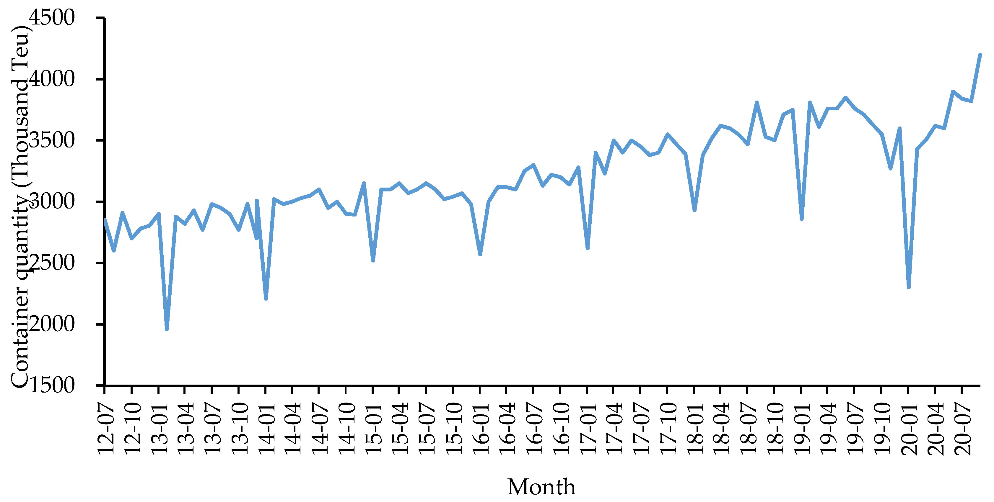
4.1.1. Data Description

The International Maritime Organization (IMO) reported that maritime transport accounts for more than 90% of global trade, which indicates that shipping is the dominant mode of transportation in global trade [44]. This empirical analysis is based on the monthly throughput data of Shanghai port from July 2012 to October 2020, as shown in Figure 3.

4.1.2. Evaluation Criteria and Indicators

In this part, the root mean square error (RMSE), absolute percentage error (APE), mean absolute percentage error (MAPE), and coefficient of determination (accuracy) are utilized to evaluate the performance of forecasting results.

$$\mathrm{RMSE}:\sqrt{\frac{1}{n}{\sum }_{t=1}^n{(y_t-y_t^{\prime })}^2},$$

(14)

$$\mathrm{APE}:{\sum }_{t=1}^n\frac{\left|y_t-y_t^{\prime }\right|}{y_t},$$

(15)

$$\mathrm{MAPE}:\frac{1}{n}{\displaystyle {\displaystyle \sum }_{t=1}^n}\frac{\left|y_t-y_t^{\prime }\right|}{y_t} ,$$

(16)

$${\mathrm{R}}^2:1-\frac{ {\sum }_1^n{\left(y_t^{\prime }-y\right)}^2 }{{\sum }_1^n{\left(y_t-\overline{y}\right)}^2},$$

(17)

where $y_t$ is the measured value, $\overline{y}$ is the average value of the measured value, $y_t^{\prime }$ is the predicted value, $\tilde{y}$ is the average value of the predicted value series, and $n$is the number of test sample sets.

4.2. Empirical Results

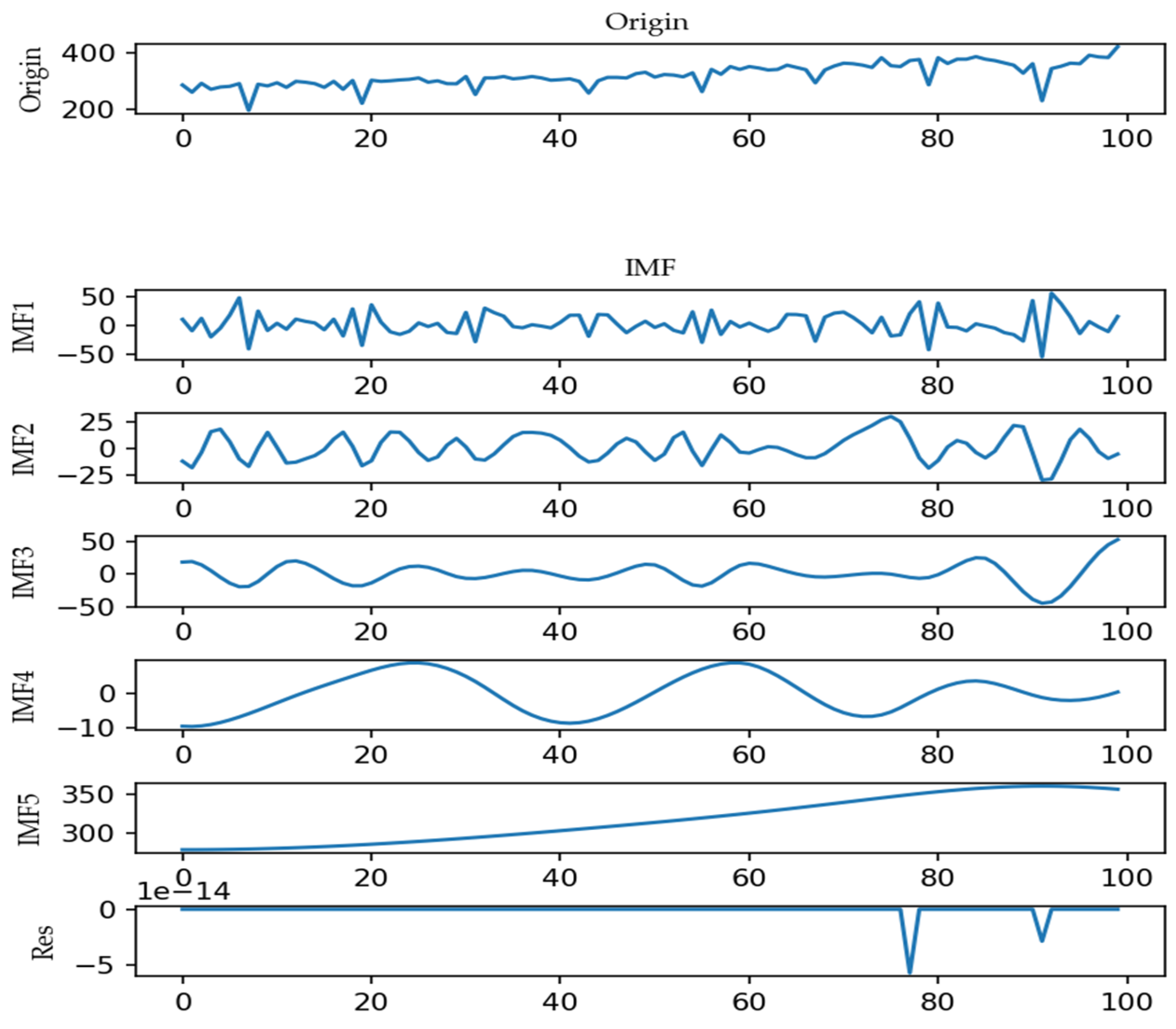
4.2.1. Data Decomposition and Event Analysis

According to the data collected from the Ministry of Transport of China, the container throughput data of Shanghai port from January 2012 to September 2020 are analyzed by EMD algorithm. The decomposition results, as shown in Figure 4, show that the container throughput fluctuation of Shanghai port implies five different scales of modes and one residual component.

The container throughput time series of Shanghai port is finally decomposed into five IMF modes and one RES. Figure 5 reflects the multi-scale fluctuation characteristics of container throughput changes, and the RES mode has no trend of variation. Therefore, the RES mode is screened. Then, this paper will test and filtrate each meaningful series, including a stationarity test, fluctuation scale analysis, and change-point test.

The non-stationary modes are removed through the stationarity test. The modes that cannot clearly reflect the fluctuation characteristics of the original data series are removed by the variance contribution rate and correlation coefficient in the fluctuation analysis. According to the screening results in

Table 2. Screening results of throughput modes.

Mode Test	IMF1	IMF2	IMF3	IMF4	IMF5
ADF test	×	√	√	√	√
fluctuation scale analysis	-	√	×	√	√

, only IMF2, IMF3, and IMF5 are left for the final change-point test. The EMD decomposition method separates the event influence factors from the original data, while the structural change-point test (ICSS–Chow test) can capture the impact of COVID-19 on the original data.

Before the change-point test, in order to match the event with the change point, we need to sort out the relevant events that affected Shanghai port after July 2012. We list the important events that may cause oscillation and fluctuation of the port throughput data, as shown in

Table 3. List of events affecting throughput of Shanghai port.

Number	Time	Events
1	2017.4–2017.5	Big congestion event
2	2019.12–2020.5	COVID-19 incident

.

According to the fluctuation characteristics of the model in

Table 4. Fluctuation analysis of IMF modes.

Index	IMF2	IMF3	IMF4	IMF5
variance contribution rate	11.16%	19.00%	2.33%	67.50%
correlation coefficient r	28.00%	35.00%	11.00%	77.00%
fluctuation cycle	3.45	6.25	14.29	long-term trend

, IMF5 can be indicated as a long-term trend mode. For the IMF2 mode, we can obtain some theoretical analyses that periodic data will have a short-term self-adjusting function [29], and we define it as short-term self-adjusting periodic fluctuation. At the same time, the period of IMF3 is 6–7 months. The port has a 6-month fluctuation, and its fluctuation magnitude also shows strong stability in the observed period [45]. This change is mainly determined by the seasonality of social production and consumption. Therefore, this paper defines the change as a seasonal period. Next, we combine ICSS with the Chow test to test the change points of IMF2, IMF3, and IMF5. We explore the impact of important events on the throughput of the upper port from a multi-scale perspective. The results are shown in

Table 5. Test results of impact of important events on port throughput fluctuation.

Number	Meaning of Mode	Impact Points Determined by ICSS	Adjusted Influence Point	Corresponding Event
IMF2	short-term self-adjusting cycle	point 94	point 92	COVID-19
IMF3	seasonal periodic fluctuation	null	null	null
IMF5	long-term trend	null	null	null

.

The results in Table 5 show that, according to the test of the ICSS algorithm, there is no structural change point in the original sequence of port throughput. The results mean that, at 95% confidence level, there is no evidence that large congestion and COVID-19 affect the throughput of Shanghai port. The results of a multi-scale time series test show that there is a change point 92 in the short-term self-adjusting period IMF2, but there is no change point in the seasonal cycle fluctuation and long-term trend. The “big congestion” does not lead to the change point in the mode. The results show that COVID-19 affects the short-term self-adjusting period of port throughput, while the “big congestion” event has no effect on the mode fluctuation of port throughput. Therefore, we can conclude that the “big congestion” can be adjusted by the port’s self-regulation system, which means the impact of the event is within the self-adjusting period and has no impact on the throughput of the port. According to official reports, the so-called “big congestion” is a misnomer. This event is due to the adjustment of the port according to the number of arriving ships, weather forecast, and dynamic conditions of each terminal. Then, each terminal operates normally and orderly with no congestion. The so-called delayed announcement issued by relevant shipping companies are the normal adjustments after the negotiation with the port. This fact is consistent with our analysis.

Because of the change point 92 in IMF2, COVID-19 has a certain effect on the fluctuation of the IMF2 mode. However, there are no change point in IMF3 and IMF5, which means that COVID-19 has no effect on the seasonal fluctuation and the long-term trend of port throughput. The above results further prove that the EMD decomposition indeed can deepen our understanding of the fluctuation law of port throughput. This paper will further analyze the difference between the IMF2 mode (short-term self-adjusting fluctuation mode) and the IMF3 mode (seasonal periodic fluctuation mode) under COVID-19. A statistical description of the data segment is shown in Figure 5.

When the amplitude of the data segment changes greatly before and after the point, we can conclude that the breakpoint causes great changes in the data. The change point of the short-term self-adjusting period mode IMF2 corresponds to the COVID-19 event. The amplitude of the two segments of the data before and after the breakpoint of IMF2 is obviously different; thus, the statistics of the IMF2 mode fluctuation, such as the difference and variance, are becoming larger. However, considering that the amount of data in the second section is small, we cannot judge the impact of the event breakpoint. Further analysis and judgment, through the comparison results of the fitting degree of normal distribution of the seasonal periodic fluctuation in IMF3, is necessary. Here, according to the experiments of D’Agostino [46], we use the skewness and kurtosis of the data segment to conduct a comprehensive test. In this test, we use the square of the skewness and kurtosis of the data segment as the statistical value to test whether the data segment conforms to a normal distribution.

We find that the skewness and slope of the two data segments in IMF2 vary greatly, compared with that in IMF3, based on

Table 6. Segmented statistical description of IMF2 and IMF3 sequences.

Mode		IMF2		IMF3
Data segment		First segment	Second segment	First segment	Second segment
general statistics	maximum	92.70	170.30	25.32	−24.22
	minimum	−89.88	−153.33	−20.55	−28.82
	median	0.22	100.78	0.34	−1.43
	average value	4.19	38.29	0.99	−27.33
	standard deviation	24.49	136.72	11.76	1.43
amplitude	maximum	84.00	5.00	74.00	0.00
	minimum	2.00	5.00	5.00	0.00
	median	43.00	5.00	39.50	0.00
normal distribution	skewness	0.87	−0.44	0.06	1.09
	kurtosis	5.47	−1.54	−0.82	0.54
	statistical value	30.70	2.56	0.67	1.47
	probability	0.00	0.19	0.06	0.06

. Meanwhile, the statistics obtained from the square of skewness and kurtosis are also greatly different. The statistical value of the second data segment follows the normal distribution at the 90% confidence level, while the first segment does not. The two data segments before and after IMF3 follow the normal distribution. As a result, it shows that the change point has an impact on IMF2, but not on IMF3. Hence, we draw the following conclusion: COVID-19 has disrupted the port’s self-adjusting function to a certain extent and affects the fluctuation pattern of the short-term self-adjusting period (IMF2). In IMF3, the change of slope and kurtosis has not changed greatly. It can be considered that the macro regulation of relevant management departments has stabilized the port throughput fluctuation of Shanghai port to a certain extent, and it represents that it makes the seasonal periodic fluctuation return to the original fluctuation state, and that the distribution is stable without breakpoints.

Based on the mode feature of throughput in Shanghai port and the empirical results of the hybrid analysis model of the impact events, we conclude that the internal fluctuation pattern of container throughput is mainly determined by the rising long-term trend, but also affected by seasonal periodic fluctuations. In addition, the port itself has a certain short-term self-regulation ability, and the effective short-term decision-making regulation can stabilize the throughput change of port containers caused by large congestion events to a certain extent. However, COVID-19 affects the normal operation of port throughput transport and, to some extent, the port’s self-adjusting function, but not the seasonal periodic fluctuations. Therefore, we can judge that the impact range of the incident is 4–6 months. The results will provide a basis for predicting the lag period of the model with the SVR model.

4.2.2. Mode Reconstruction and Integrated Forecasting

Through screening analysis, we divide the components into two groups and predict them with SVR and ARIMA, respectively. SVR is improved based on the impact event analysis. Therefore, IMF2, IMF3, and IMF5 are predicted by SVR. At the same time, this paper also utilizes RES to improve the forecasting accuracy. IMF3 and IMF4, without event analysis, were predicted by ARIMA.

To reduce the observation by reducing the components, we use the Pearson product–moment correlation coefficient to calculate the contribution rate of each intrinsic mode component for component reconstruction, where all intrinsic mode components are evaluated by selecting the appropriate evaluating indicators. It can filter out high-frequency noise and trend terms. Considering the great differences between modes in this paper, the contribution rate threshold value is set to 0.2 (generally 0.01), as shown in Figure 5.

Compared with the threshold of contribution rate, the IMF components larger than the threshold are IMF2, IMF3, IMF4, and IMF5. Considering that they are in different forecasting groups, we integrate IMF3, IMF4, and IMF5 into a new IMF3, and IMF2 is not reconstructed. The new component mode is shown in Figure 6.

In this section, the non-stationary mode IMF1, and the mode IMF2 with change points, are predicted by the SVR model, while the reconstructed model IMF3 is predicted by the ARIMA model. Firstly, we set the range of the SVR optimal parameter combination $\left(\gamma ,{\sigma }^2\right)$ as $\left[0.01,1000\right]$. In the ARIMA model, the optimal model of each training sample determines the optimal value of parameter $\left(\mathrm{p},\mathrm{q}\right)$ by minimizing the BIC criterion (Bayesian Information Criterion). Then, the EEAS (EMD-Event Analysis-Arima-SVR), E-S (EMD-SVR), SVR, and ARIMA models are used to predict port throughout from January 2020 to October 2020. The selection of the SVR forecasting lag period is defined according to the event analysis results. In the previous section, we obtained an impact range of 4–6 months; therefore, in order to avoid the impact of change points on the forecasting model, we set the lag period as $d=7$ and compare the forecasting performance with other forecasting technologies. The forecasting performance of different models is shown in

Table 7. Model test results with training size of 0.75.

Size = 0.75	Tested Index	RMSE	APE	MAPE	Coefficient of Determination	Running Time (/s)
tested model	EPSA (d = 7)	11.62	0.23	0.02	0.94	2028.07
	ES (d = 7)	19.78	0.40	0.04	0.83	4147.40
	SVR (d = 7)	15.95	0.25	0.03	0.89	369.04
	ARIMA	24.09	0.56	0.06	0.75	218.77

.

Compared with other forecasting models, we can conclude that the error level of the EEAS model$\left(d=7\right)$constructed in this paper is relatively smaller, and that the determination coefficient (forecasting accuracy) is higher. Therefore, we can judge that the port forecasting accuracy of the EEAS decomposition–integration model is higher than other single forecasting models, and that the running time of EEAS is lower than the ES requirement. Since the ES model uses the SVR model for training and forecasting all modes, the EEAS model only predicts non-stationary linear modes, which greatly shortens the running time and reduces the energy consumption of the forecasting operation. At the same time, the EEAS, E-S (EMD-SVR), and SVR models are better than ARIMA, which cannot solve the forecasting problem with nonlinear stationary data. However, the SVR can predict non-stationary and stationary data through training data. Thus, based on decomposition–integration theory, the forecasting performance of the EEAS model is obviously better than other single forecasting models.

To eliminate the influence of training size and verify the reliability of taking value $d=7$, so as to enhance the interpretability and generality of the research, we will use the SVR model (E-S, SVR) to carry out a comparative experimental analysis under different training sizes and conditions. The value $d=7$ is determined according to the mixed-event analysis model. The experiment will be divided into two parts: experimental verification and experimental result analysis. In this paper, the E-S (EMD-SVR) and SVR models will be used to predict the above data in different training sizes $\left(\mathrm{i}.\mathrm{e}., 0.2, 0.25, 0.3\right)$ and different lag periods $\left(\mathrm{i}.\mathrm{e}., d=4,7,8\right)$. The results are shown in Figure 7.

Figure 7 reflects the fitting degree between the predicted value and the real value of each model. We select the evaluation index and accuracy coefficient of the forecasting model to further conduct a more specific numerical analysis on the forecasting results. In Figure 7, the higher the value, the better the forecasting effect, and the closer the predicted value is to the real value. We calculate the coefficient of determination of each model in Figure 8.

In Figure 8, the darker the color, the smaller value and the worse the forecasting performance. In Figure 8, when $d=7$, no matter how the size changes, the accuracy coefficient is very high. This means that the consistency between the predicted value and the real value is very high. The accuracy coefficient of the forecasting model with $d=4.8$ is lower than $0.8,$ which indicates that the forecasting performance of the forecasting model will change greatly when the training size changes. Therefore, the forecasting effect when $d=7$ is not affected by the training size, and the efficiency is better than that when $d=4.8$. It is concluded that the data lag period $d$, defined by the event analysis, makes the SVR model less vulnerable to the influence of training size, thus improving the overall forecasting performance.

To further explore the main mode affecting the forecasting results, we predict each mode separately in different $d$ scenarios with training $\mathrm{size}\mathrm{equals}0.8$ (the fitting degree of forecasting results under this size is low for many times). The comparison results show that the low forecasting accuracy of the decomposition–integration model is mainly due to the mode IMF1. The specific results are shown in Figure 9.

In Figure 9, the fitting degree is the worst under the scenario when $d=4.8$ (yellow and black), and the fitting degree when $d=7$ (red) is very good. Among them$,d=4.8$are the control parameters, and $d=7$ is selected by the analysis results in Section 3. Considering that IMF1 is composed of non-stationary data, the selection of lag period $d$ will effectively improve the forecasting accuracy of non-stationary mode data and is not easily affected by the change of training size.

5. Conclusions and Future Work

COVID-19 has cast a complex impact on container throughput at ports, posing a huge challenge to accurate forecasting. With the impact of this major event, it is an important task to develop an effective container throughput forecasting model. This paper proposes a new forecasting model (EMD-Event Analysis-ARIMA-SVR (EEAS)) based on the background of COVID-19.

Firstly, EMD is used to decompose the sample data of port container throughput into multiple components. Secondly, fluctuation scale analysis is carried out to accurately capture the characteristics of the components. Subsequently, we tailor the forecasting model for every component based on the mode analysis. Finally, the forecasting results of all the components are combined into one aggregated output. Based on the forecasting results of the container throughput of Shanghai port, we can conclude that the proposed model performs better than EMD-SVR, SVR, and ARIMA.

This paper proposes a novel decomposition–ensemble forecasting framework for port container throughput in the context of major events. In addition, event analysis is introduced into the decomposition–ensemble forecasting model. Based on the proposed forecasting framework, future research can flexibly tailor appropriate forecasting models according to different data characteristics in the context of major events. This paper provides an analytical tool for impact analysis and forecasting in the context of COVID-19, and provides a powerful reference for port production, operation, and investment development planning in the context of major events. The limitation of this study lies in that the proposed model is tailored to capture the impacts of major events, and the improvement of forecasting accuracy under stationary scenarios is not significant enough, compared with traditional models. In addition to container throughput forecasting, the proposed methodology can be extended into other difficult forecasting tasks, such as material demand after major disasters.

References

1. Notteboom, T. The adaptive capacity of container ports in an era of mega vessels: The case of upstream seaports Antwerp and Hamburg. J. Transp. Geogr. 2016, 54, 295–309. [Google Scholar] [CrossRef]
2. Notteboom, T.; Pallis, T.; Rodrigue, J.P. Disruptions and resilience in global container shipping and ports: The COVID-19 pandemic versus the 2008–2009 financial crisis. Marit. Econ. Logist. 2021, 23, 179–210. [Google Scholar] [CrossRef]
3. World Health Organization (WHO). Available online: https://www.who.int/zh/news/item/29-06-2020-covidtimeline (accessed on 10 February 2022).
4. McKibbin, W.; Fernando, R. The Global Macroeconomic Impacts of COVID-19: Seven Scenarios. Asian Econ. Pap. 2021, 20, 1–30. [Google Scholar] [CrossRef]
5. Depellegrin, D.; Bastianini, M.; Fadini, A.; Menegon, S. The effects of COVID-19 induced lockdown measures on maritime settings of a coastal region. Sci. Total Environ. 2020, 740, 140123. [Google Scholar] [CrossRef] [PubMed]
6. Chou, C.C.; Chu, C.W.; Liang, G.S. A modified regression model for forecasting the volumes of Taiwan’s import containers. Math. Comput. Model. 2008, 47, 797–807. [Google Scholar] [CrossRef]
7. Rashed, Y.; Meersman, H.; De Voorde, E.V.; Vanelslander, T. Short-term forecast of container throughout: An ARIMA-intervention model for the port of Antwerp. Marit. Econ. Logist. 2017, 19, 749–764. [Google Scholar] [CrossRef]
8. Farhan, J.; Ong, G.P. Forecasting seasonal container throughput at international ports using SARIMA models. Marit. Econ. Logist. 2018, 20, 131–148. [Google Scholar] [CrossRef]
9. Ruiz-Aguilar, J.J.; Turias, I.J.; Jimenez-Come, M.J. Hybrid approaches based on SARIMA and artificial neural networks for inspection time series forecasting. Transp. Res. Part E Logist. Transp. Rev. 2014, 67, 1–13. [Google Scholar] [CrossRef]
10. Schulze, P.M.; Prinz, A. Forecasting container transshipment in Germany. Appl. Econ. 2009, 41, 2809–2815. [Google Scholar] [CrossRef] [Green Version]
11. Fung, M.K. Forecasting in Hong Kong’s container throughput: An error-correction model. J. Forecast. 2002, 21, 69–80. [Google Scholar] [CrossRef]
12. Munim, Z.H.; Schramm, H.J. Forecasting container shipping freight rates for the Far East-Northern Europe trade lane. Marit. Econ. Logist. 2016, 19, 106–125. [Google Scholar] [CrossRef]
13. Veenstra, A.W.; Haralambides, H.E. Multivariate autoregressive models for forecasting seaborne trade flows. Transp. Res. Part E Logist. Transp. Rev. 2001, 37, 311–319. [Google Scholar] [CrossRef]
14. Gao, Y.; Luo, M.F.; Zou, G.H. Forecasting with model selection or model averaging: A case study for monthly container port throughput. Transp. A 2016, 12, 366–384. [Google Scholar] [CrossRef]
15. Peng, W.Y.; Chu, C.W. A comparison of univariate methods for forecasting container throughput volumes. Math. Comput. Model. 2009, 50, 1045–1057. [Google Scholar] [CrossRef]
16. Guo, Z.X.; Le, W.W.; Wu, Y.K.; Wang, W. A multi-step approach framework for freight forecasting of river-sea direct transport without direct historical data. Sustainability 2019, 11, 4252. [Google Scholar] [CrossRef] [Green Version]
17. Ding, M.J.; Zhang, S.Z.; Zhong, H.D.; Wu, Y.H.; Zhang, L.B. A prediction model of the sum of container based on combined BP neural network and SVM. J. Inf. Processing Syst. 2019, 15, 305–319. [Google Scholar]
18. He, C.; Wang, H.P. Container Throughput Forecasting of Tianjin-Hebei Port Group Based on Grey Combination Model. J. Math. 2021, 2021, 8877865. [Google Scholar] [CrossRef]
19. Jing, G.; Li, M.W.; Dong, Z.H.; Liao, Y.S. Port throughput forecasting by MARS-RSVR with chaotic simulated annealing particle swarm optimization algorithm. Neurocomputing 2015, 147, 239–250. [Google Scholar]
20. Xiao, J.; Xiao, Y.; Fu, J.L.; Lai, K.K. A transfer forecasting model for container throughput guided by discrete PSO. J. Syst. Sci. Complex. 2014, 27, 181–192. [Google Scholar] [CrossRef]
21. Liu, S.; Tian, L.X.; Huang, Y.S. A comparative study on prediction of throughput in coal ports among three models. Int. J. Mach. Learn. Cybern. 2014, 5, 125–133. [Google Scholar] [CrossRef]
22. Milenkovic, M.; Milosavljevic, N.; Bojovic, N.; Val, S. Container flow forecasting through neural networks based on metaheuristics. Oper. Res. 2021, 21, 965–997. [Google Scholar] [CrossRef]
23. Yu, L.A.; Wang, Z.S.; Tang, L. A decomposition–ensemble model with data-characteristic-driven reconstruction for crude oil price forecasting. Appl. Energy 2015, 156, 251–267. [Google Scholar] [CrossRef]
24. Tang, L.; Yu, L.; Wang, S.; Li, J.P.; Wang, S.Y. A novel hybrid ensemble learning paradigm for nuclear energy consumption forecasting. Appl. Energy 2012, 93, 432–443. [Google Scholar] [CrossRef]
25. Hang, A.Q.; Lai, K.; Li, Y.H.; Wang, S.Y. Forecasting Container Throughput of Qingdao Port with a Hybrid Model. J. Syst. Sci. Complex. 2015, 28, 105–121. [Google Scholar] [CrossRef]
26. Yu, L.; Liang, S.; Chen, R. Predicting monthly bio fuel production using a hybrid ensemble forecasting methodology. Int. J. Forecast. 2019, 38, 3–20. [Google Scholar] [CrossRef]
27. Xie, G.; Wang, S.Y.; Zhao, Y.X.; Lai, K.K. Hybrid approaches based on LSSVR model for container throughput forecasting: A comparative study. Appl. Soft Comput. 2013, 13, 2232–2241. [Google Scholar] [CrossRef]
28. Yu, L.A.; Zhao, Y.; Tang, L. Ensemble Forecasting for Complex Time Series Using Sparse Representation and Neural Networks. J. Forecast. 2016, 36, 122–138. [Google Scholar] [CrossRef]
29. Jianwei, E.; Bao, Y.L.; Ye, J.M. Crude oil price analysis and forecasting based on variational mode decomposition and independent component analysis. Physical A 2017, 484, 412–427. [Google Scholar]
30. Yu, L.; Wang, S.Y.; Lai, K.K. Forecasting crude oil price with an EMD-based neural network ensemble learning paradigm. Energy Econ. 2008, 30, 2623–2635. [Google Scholar] [CrossRef]
31. Huang, N.E.; Shen, Z.; Long, S.R. The empirical mode decomposition and the Hilbert spectrum for nonlinear and non-stationary time series analysis. Proc. R. Soc. A-Math. Phys. Eng. Sci. 1998, 454, 903–995. [Google Scholar] [CrossRef]
32. Zhang, X.; Yu, L.; Wang, S.Y.; Lai, K.K. Estimating the impact of extreme events on crude oil price: An EMD-based event analysis method. Energy Econ. 2009, 31, 768–778. [Google Scholar] [CrossRef]
33. Zhang, X.; Lai, K.K.; Wang, S.Y. A new approach for crude oil price analysis based on Empirical Mode Decomposition. Energy Econ. 2008, 30, 905–918. [Google Scholar] [CrossRef]
34. Inclán, C.; Tiao, G.C. Use of Cumulative Sums of Squares for Retrospective Detection of Changes of Variance. J. Am. Stat. Assoc. 1994, 89, 913–923. [Google Scholar]
35. Wu, B.R.; Wang, L.; Lv, S.X.; Zeng, Y.R. Effective crude oil price forecasting using new text-based and big-data-driven model. Measurement 2021, 168, 108468. [Google Scholar] [CrossRef]
36. Wu, B.R.; Wang, L.; Wang, S.R.; Zeng, Y.R. Forecasting the US oil markets based on social media information during the COVID-19 pandemic. Energy 2021, 226, 120403. [Google Scholar] [CrossRef]
37. Weng, F.T.; Zhang, H.W.; Yang, C. Volatility forecasting of crude oil futures based on a genetic algorithm regularization online extreme learning machine with a forgetting factor: The role of news during the COVID-19 pandemic. Resour. Policy 2021, 73, 102148. [Google Scholar] [CrossRef]
38. Stifanic, D.; Musulin, J.; Miocevic, A.; Segota, S.B.; Subic, R.; Car, Z. Impact of COVID-19 on Forecasting Stock Prices: An Integration of Stationary Wavelet Transform and Bidirectional Long Short-Term Memory. Complexity 2020, 2020, 1846926. [Google Scholar] [CrossRef]
39. Koyuncu, K.; Tavacioglu, L.; Gokmen, N.; Arican, U.C. Forecasting COVID-19 impact on RWI/ISL container throughput index by using SARIMA models. Marit. Policy Manag. 2021, 48, 1096–1108. [Google Scholar] [CrossRef]
40. Tang, L.; Dai, W.; Yu, L.A. A Novel CEEMD-Based EELM Ensemble Learning Paradigm for Crude Oil Price Forecasting. Int. J. Inf. Technol. Decis. Mak. 2015, 14, 141–169. [Google Scholar] [CrossRef]
41. Rodgers, L.; Nicewander, W.A. Thirteen ways to look at the correlation coefficient. J. Stat. 1988, 42, 59–66. [Google Scholar] [CrossRef]
42. Box, G.; Pierce, D.A. Distribution of Residual Autocorrelations in ARIMA Time Series Models. J. Am. Stat. Assoc. 1970, 72, 397–402. [Google Scholar]
43. Bousquet, O. New approaches to statistical learning theory. Ann. Inst. Stat. Math. 2003, 55, 371–389. [Google Scholar] [CrossRef]
44. Xie, G.; Yue, W.; Wang, S. Energy efficiency decision and selection of main engines in a sustainable shipbuilding supply chain. Transp. Res. Part D Transp. Environ. 2017, 53, 290–305. [Google Scholar] [CrossRef]
45. Twrdy, E.; Batista, M. Modeling of container throughput in Northern Adriatic ports over the period 1990-2013. J. Transp. Geogr. 2016, 52, 131–142. [Google Scholar] [CrossRef]
46. D’Agostino, R.B. An omnibus test of normality for moderate and large size samples. Biometrika 1971, 2, 341–348. [Google Scholar] [CrossRef]
Figure 1. Model framework.
Sustainability 14 02990 g001
Figure 2. EMD decomposition flow chart.
Sustainability 14 02990 g002
Figure 3. Container throughput of Shanghai port.
Sustainability 14 02990 g003
Figure 4. Modes of container throughput.
Sustainability 14 02990 g004
Figure 5. IMF contribution rate.
Sustainability 14 02990 g005
Figure 6. Mode reconstruction.
Sustainability 14 02990 g006
Figure 7. Forecasting results with different training sizes (10,000 TEUs).
Sustainability 14 02990 g007aSustainability 14 02990 g007b
Figure 8. Thermal spectrum of precision coefficient.
Sustainability 14 02990 g008
Figure 9. Comparison of IMF1.
Sustainability 14 02990 g009