
House Prices and Marriage in Spain


Abstract
:1. Introduction
2. Materials and Methods
2.1. Literature Review
2.2. Data
2.3. Theoretical Model
2.4. Empirical Models
3. Results
3.1. Regional Results
3.2. Local Results
4. Discussion
5. Conclusions
Funding
Institutional Review Board Statement
Informed Consent Statement
Data Availability Statement
Conflicts of Interest
Appendix A

| Variable | Mean | Standard Deviation | Minimum | Maximum |
|---|---|---|---|---|
| Marriage rate (regional data) | 4.073 | 0.885 | 2.042 | 6.226 |
| Marriage rate (local data) | 3.895 | 1.019 | 0.598 | 9.820 |
| House price (regional data) | 1162.902 | 520.708 | 383.2 | 3045.6 |
| House price (local data) | 1580.679 | 660.446 | 519.575 | 3899.4 |
| Regional unemployment rate | 16.395 | 7.794 | 2.996 | 42.303 |
| Regional inflation rate | 2.299 | 1.517 | −1.575 | 5.908 |
| Regional % female population with some college | 20.352 | 7.476 | 5.722 | 54.316 |
References
- Gholipour, H.F.; Farzanegan, M.R. Marriage crisis and housing costs: Empirical evidence from provinces of Iran. J. Policy Modeling 2015, 37, 107–123. [Google Scholar] [CrossRef] [Green Version]
- Grossbard-Schectman, S. On the Economics of Marriage; Routledge: New York, NY, USA, 2019. [Google Scholar]
- Becker, G.S. A theory of marriage: Part I. J. Political Econ. 1973, 81, 813–846. [Google Scholar] [CrossRef]
- Shore, S.H. For better, for worse: Intra-household risk-sharing over the business cycle. Rev. Econ. Stat. 2009, 92, 536–548. [Google Scholar] [CrossRef]
- Stevenson, B.; Wolfers, J. Marriage and divorce: Changes and their driving forces. J. Econ. Perspect. 2007, 21, 27–52. [Google Scholar] [CrossRef] [Green Version]
- Grossbard, S. The Marriage Motive: A Price Theory of Marriage: How Marriage Markets Affect Employment, Consumption, and Savings; Springer: New York, NY, USA, 2015. [Google Scholar]
- Langlais, E. On unilateral divorce and the “selection of marriages” hypothesis. Louvain Econ. Rev. 2010, 76, 229–256. [Google Scholar] [CrossRef] [Green Version]
- Ahn, N.; Mira, P. Job Bust, Baby Bust?: Evidence from Spain. J. Popul. Econ. 2001, 14, 505–521. [Google Scholar] [CrossRef]
- Parreño Castellano, J.M.; Domínguez Mujica, J.; Armengol Martín, M.T.; Boldú Hernández, J.; Pérez García, T. Real estate dispossession and evictions in Spain: A theoretical geographical approach. Boletín Asoc. Geógrafos Españoles 2019, 80, 2602. [Google Scholar] [CrossRef] [Green Version]
- Romero, J.; Jiménez, F.; Villoria, M. (Un)sustainable territories: Causes of the speculative bubble in Spain (1996–2010) and its territorial, environmental, and sociopolitical consequences. Environ. Plan. C Gov. Policy 2012, 30, 467–486. [Google Scholar] [CrossRef]
- Blanco, F.; Martín, V.; Vazquez, G. Regional house price convergence in Spain during the housing boom. Urban Stud. 2016, 53, 775–798. [Google Scholar] [CrossRef]
- Ogburn, W.F.; Thomas, D.S. The influence of the business cycle on certain social conditions. J. Am. Stat. Assoc. 1922, 18, 324–340. [Google Scholar] [CrossRef]
- Stouffer, S.A.; Spencer, L.M. Marriage and divorce in recent years. Ann. Am. Acad. Political Soc. Sci. 1936, 188, 56–69. [Google Scholar] [CrossRef]
- Silver, M. Births, marriages, and business cycles in the United States. J. Political Econ. 1965, 73, 237–255. [Google Scholar] [CrossRef]
- Browning, M.; Chiappori, P.-A.; Weiss, Y. Economics of the Family; Cambridge University Press: Cambridge, NY, USA, 2014. [Google Scholar]
- Borsch-Supan, A. Household formation, housing prices, and public policy impacts. J. Public Econ. 1986, 30, 145–164. [Google Scholar] [CrossRef]
- Edin, K.; Reed, J. Why don’t they just get married? Barriers to marriage amongst the disadvantaged. Future Child. 2005, 15, 117–137. [Google Scholar] [CrossRef]
- Wrenn, D.H.; Yi, J.; Zhang, B. House prices and marriage entry in China. Reg. Sci. Urban Econ. 2019, 74, 118–130. [Google Scholar] [CrossRef]
- Hu, M.; Wu, L.; Xiang, G.; Zhong, S. Housing prices and the probability of marriage among the young: Evidence from land reform in China. Int. J. Emerg. Mark. 2021. [Google Scholar] [CrossRef]
- Ermisch, J.; Di Salvo, P. The economic determinants of young people’s household formation. Economica 1997, 64, 627–644. [Google Scholar] [CrossRef]
- Haurin, D.R.; Hendershott, P.H.; Kim, D. The impact of real rents and wages on household formation. Rev. Econ. Stat. 1993, 75, 284–293. [Google Scholar] [CrossRef]
- Mulder, C.H.; Billari, F.C. Homeownership regimes and low fertility. Hous. Stud. 2010, 25, 527–541. [Google Scholar] [CrossRef]
- Clark, W.A.V.; Deurloo, M.C.; Dieleman, F.M. Tenure changes in the context of micro level family and macro level economic shifts. Urban Stud. 1994, 31, 137–154. [Google Scholar] [CrossRef]
- Clark, W.A.V.; Dieleman, F.M. Households and Housing: Choice and Outcomes in the Housing Market; Centre for Urban Policy Research: New Brunswick, NJ, USA, 1996. [Google Scholar]
- Kendig, H.L. Housing careers, life cycle and residential mobility: Implications for the housing market. Urban Stud. 1984, 21, 271–283. [Google Scholar] [CrossRef]
- Montgomery, M. Household formation and home-ownership in France. In Demographic Applications of Event History Analysis; Trussell, J., Hankinson, R., Tilton, J., Eds.; Clarendon Press: Oxford, UK, 1992; pp. 94–119. [Google Scholar]
- Feijten, P.; Mulder, C.H. The timing of household events and housing events in the Netherlands: A longitudinal perspective. Hous. Stud. 2002, 17, 773–792. [Google Scholar] [CrossRef]
- Mulder, C.H.; Wagner, M. First-time home-ownership in the family life course: A West German-Dutch comparison. Urban Stud. 1998, 35, 687–713. [Google Scholar] [CrossRef]
- Su, C.-W.; Khan, K.; Hao, L.-N.; Tao, R.; Dumitrescu Peculea, A. Do house prices squeeze marriages in China? Econ. Res.-Ekon. Istraživanja 2020, 33, 1419–1440. [Google Scholar] [CrossRef]
- Martín, A.; Moral-Benito, E.; Schmitz, T. The Financial Transmission of Housing Bubbles: Evidence from Spain. American Economic Review 2021, 111, 1013–1053. [Google Scholar] [CrossRef]
- Weiss, Y. The formation and dissolution of families: Why marry? Who marries whom? And what happens upon divorce. Handb. Popul. Fam. Econ. 1997, 1, 81–123. [Google Scholar]
- Yi, J.; Zhang, J. The effect of house price on fertility: Evidence from Hong Kong. Econ. Inq. 2009, 48, 635–650. [Google Scholar] [CrossRef]
- Ruzhi, X.U.; Khan, K.; Moldovan, N.C.; Iosif, A. Do house prices and marriages move together in China? Econ. Comput. Econ. Cybern. Stud. Res. 2019, 53, 59–78. [Google Scholar] [CrossRef]
- Easterlin, R.A. Birth and Fortune: The Impact of Numbers on Personal Welfare; Basic Books: New York, NY, USA, 1980. [Google Scholar]
- Hughes, M.E. What Money Can Buy: The Relationship between Marriage and Home Ownership in the United States; Duke University: Durham, NC, USA, 2004. [Google Scholar]
- González-Val, R.; Marcén, M. Unemployment, Marriage and Divorce. Appl. Econ. 2018, 50, 1495–1508. [Google Scholar] [CrossRef] [Green Version]
- Schellekens, J.; Gliksberg, D. Inflation and Marriage in Israel. J. Fam. Hist. 2013, 38, 78–93. [Google Scholar] [CrossRef]
- Lopez, C.; Papell, D.H. Convergence of Euro area inflation rates. J. Int. Money Financ. 2012, 31, 1440–1458. [Google Scholar] [CrossRef]
- Torr, B.M. The Changing Relationship between Education and Marriage in the United States, 1940–2000. J. Fam. Hist. 2011, 36, 483–503. [Google Scholar] [CrossRef] [PubMed]
- Gutiérrez-Domènech, M. The impact of the labour market on the timing of marriage and births in Spain. J. Popul. Econ. 2008, 21, 83–110. [Google Scholar] [CrossRef] [Green Version]
- Connolly, M. Some like it mild and not too wet: The influence of weather on subjective well-being. J. Happiness Stud. 2013, 14, 457–473. [Google Scholar] [CrossRef] [Green Version]
- Arellano, M.; Bond, S. Some tests of specification for panel data: Monte Carlo evidence and an application to employment equations. Rev. Econ. Stud. 1991, 58, 277–297. [Google Scholar] [CrossRef] [Green Version]
- Méndez, R. Ciudades en Venta; PUV Universitat de València: Valencia, Spain, 2019. [Google Scholar]
- González-Val, R. The effects of the 2012 Spanish law reform to protect mortgage debtors. Hous. Policy Debate 2021, 31, 239–253. [Google Scholar] [CrossRef]
- Akin, O.; Montalvo, J.; Villar, J.G.; Peydró, J.-L.; Raya, J. The real estate and credit bubble: Evidence from Spain. SERIEs-J. Span. Econ. Assoc. 2014, 5, 223–243. [Google Scholar] [CrossRef] [Green Version]
- García, M. The breakdown of the Spanish urban growth model: Social and territorial effects of the global crisis. Int. J. Urban Reg. Res. 2010, 34, 967–980. [Google Scholar] [CrossRef] [Green Version]
- Clark, W.A.V. Do women delay family formation in expensive housing markets? Demogr. Res. 2012, 27, 1–24. [Google Scholar] [CrossRef] [Green Version]
- Enström Öst, C. Housing and children: Simultaneous decisions?—A cohort study of young adults’ housing and family formation decision. J. Popul. Econ. 2011, 25, 349–366. [Google Scholar]
- Durlauf, S.N. Manifesto for a growth econometrics. J. Econom. 2001, 100, 65–69. [Google Scholar] [CrossRef] [Green Version]

| Regional Data | Local Data | |||
|---|---|---|---|---|
| Year | Marriage Rate | House Price | Marriage Rate | House Price |
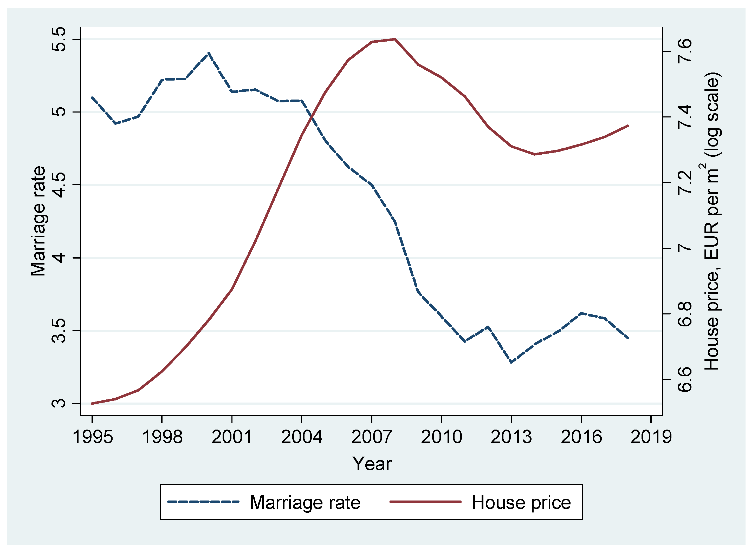
| 1995 | 4.77 | 581.60 | ||
| 1996 | 4.62 | 591.37 | ||
| 1997 | 4.63 | 604.27 | ||
| 1998 | 4.81 | 637.15 | ||
| 1999 | 4.84 | 697.38 | ||
| 2000 | 4.98 | 782.21 | ||
| 2001 | 4.70 | 877.42 | ||
| 2002 | 4.78 | 984.78 | ||
| 2003 | 4.73 | 1108.66 | ||
| 2004 | 4.71 | 1271.78 | ||
| 2005 | 4.49 | 1439.82 | 4.98 | 1785.15 |
| 2006 | 4.35 | 1598.26 | 4.80 | 1986.84 |
| 2007 | 4.25 | 1690.56 | 4.68 | 2135.71 |
| 2008 | 4.03 | 1705.13 | 4.34 | 2119.42 |
| 2009 | 3.58 | 1581.79 | 3.82 | 1903.18 |
| 2010 | 3.40 | 1538.93 | 3.59 | 1792.34 |
| 2011 | 3.21 | 1468.96 | 3.42 | 1660.82 |
| 2012 | 3.34 | 1361.19 | 3.52 | 1514.77 |
| 2013 | 3.03 | 1260.83 | 3.26 | 1335.25 |
| 2014 | 3.20 | 1213.63 | 3.44 | 1221.03 |
| 2015 | 3.29 | 1216.32 | 3.58 | 1204.55 |
| 2016 | 3.41 | 1220.50 | 3.75 | 1209.07 |
| 2017 | 3.35 | 1230.06 | 3.72 | 1248.82 |
| 2018 | 3.25 | 1247.09 | 3.58 | 1325.80 |
| (1) | (2) | (3) | |
|---|---|---|---|
| ln(House price) | −0.481 *** | −0.488 *** | −0.525 *** |
| (0.114) | (0.125) | (0.182) | |
| Unemployment rate | −0.043 *** | −0.038 *** | |
| (0.007) | (0.006) | ||
| Inflation rate | 0.169 *** | 0.091 ** | |
| (0.016) | (0.037) | ||
| % female population with some college | −0.004 | −0.005 | |
| (0.009) | (0.005) | ||
| Weather controls | N | Y | Y |
| Regional fixed effects | N | N | Y |
| Year fixed effects | N | N | Y |
| R2 | 0.058 | 0.408 | 0.914 |
| Mean VIF | 1.000 | 2.500 | 7.200 |
| Observations | 1200 | 1200 | 1200 |
| All Regions | Excluding Barcelona and Madrid | Coastal Regions | Inland Regions | |
|---|---|---|---|---|
| (1) | (2) | (3) | (4) | |
| Marriage rate t-1 | 0.617 *** | 0.632 *** | 0.867 *** | 0.559 *** |
| (0.044) | (0.043) | (0.034) | (0.059) | |
| ln(House price) | −0.846 *** | −0.800 *** | −0.523 *** | −0.362 ** |
| (0.116) | (0.118) | (0.113) | (0.162) | |
| Unemployment rate | −0.011 *** | −0.010 ** | −0.001 | −0.006 |
| (0.004) | (0.004) | (0.005) | (0.004) | |
| Inflation rate | 0.029 | 0.031 | 0.008 | 0.042 * |
| (0.021) | (0.022) | (0.024) | (0.023) | |
| % female population with some college | −0.003 | −0.003 | −0.004 | −0.002 |
| (0.003) | (0.003) | (0.003) | (0.002) | |
| Weather controls | Y | Y | Y | Y |
| Year fixed effects | Y | Y | Y | Y |
| AR(2), p-value | 0.055 | 0.030 | 0.040 | 0.200 |
| Hansen test, p-value | 0.999 | 0.999 | 0.999 | 0.999 |
| Regions | 50 | 48 | 22 | 28 |
| Observations | 1150 | 1104 | 506 | 644 |
| All Cities | Excluding Barcelona and Madrid | Excluding Capital Cities | |
|---|---|---|---|
| (1) | (2) | (3) | |
| Local marriage rate t−1 | 0.166 *** | 0.165 *** | 0.177 *** |
| (0.032) | (0.032) | (0.034) | |
| ln(Local house price) | −0.487 ** | −0.501 ** | −0.550 ** |
| (0.225) | (0.228) | (0.235) | |
| Regional unemployment rate | −0.057 *** | −0.057 *** | −0.058 *** |
| (0.008) | (0.008) | (0.009) | |
| Regional inflation rate | 0.055 | 0.055 | 0.077 * |
| (0.035) | (0.035) | (0.044) | |
| Regional % female population with some college | −0.003 | −0.003 | −0.004 |
| (0.005) | (0.005) | (0.007) | |
| Regional weather controls | Y | Y | Y |
| Year fixed effects | Y | Y | Y |
| AR(2), p-value | 0.427 | 0.109 | 0.165 |
| Hansen test, p-value | 0.106 | 0.100 | 0.585 |
| Cities | 282 | 280 | 232 |
| Observations | 3378 | 3354 | 2778 |
Publisher’s Note: MDPI stays neutral with regard to jurisdictional claims in published maps and institutional affiliations. |
© 2022 by the author. Licensee MDPI, Basel, Switzerland. This article is an open access article distributed under the terms and conditions of the Creative Commons Attribution (CC BY) license (https://creativecommons.org/licenses/by/4.0/).
Share and Cite
González-Val, R. House Prices and Marriage in Spain. Sustainability 2022, 14, 2848. https://doi.org/10.3390/su14052848
González-Val R. House Prices and Marriage in Spain. Sustainability. 2022; 14(5):2848. https://doi.org/10.3390/su14052848
Chicago/Turabian StyleGonzález-Val, Rafael. 2022. "House Prices and Marriage in Spain" Sustainability 14, no. 5: 2848. https://doi.org/10.3390/su14052848
APA StyleGonzález-Val, R. (2022). House Prices and Marriage in Spain. Sustainability, 14(5), 2848. https://doi.org/10.3390/su14052848