Transition State Matrices Approach for Trajectory Segmentation Based on Transport Mode Change Criteria

Abstract

Identifying distribution of users’ mobility is an essential part of transport planning and traffic demand estimation. With the increase in the usage of mobile devices, they have become a valuable source of traffic mobility data. Raw data contain only specific traffic information, such as position. To extract additional information such as transport mode, collected data need to be further processed. Trajectory needs to be divided into several meaningful consecutive segments according to some criteria to determine transport mode change point. Existing algorithms for trajectory segmentation based on the transport mode change most often use predefined knowledge-based rules to create trajectory segments, i.e., rules based on defined maximum pedestrian speed or the detection of pedestrian segment between two consecutive transport modes. This paper aims to develop a method that segments trajectory based on the transport mode change in real time without preassumed rules. Instead of rules, transition patterns are detected during the transition from one transport mode to another. Transition State Matrices (TSM) were used to automatically detect the transport mode change point in the trajectory. The developed method is based on the sensor data collected from mobile devices. After testing and validating the method, an overall accuracy of $98\%$ and $96\%$, respectively, was achieved. As higher accuracy of trajectory segmentation means better and more homogeneous data, applying this method during the data collection adds additional value to the data.

1. Introduction

In many traffic management applications, data collected through sensor technologies provide a means for estimating traffic demand and transport planning. Recognition of daily transport activities has several applications, such as educating users with the aim of changing their behavior patterns or to encourage healthier lifestyle. In addition, applications that track user mobility are helping to plan public urban transportation, track vehicle traffic, and support smart parking [1].

Data collected from mobile devices are time series of sensor values recorded during user movement through the traffic network. The collected data do not contain additional information such as transport mode, so further processing has to be applied to extract such data from the collected data set. With the increase in machine learning methods, various methods are applied on sensor-based data to obtain additional information such as human activities [2], transport modes [3] or congestion zones [4]. The additional information added to a large amount of data provide a base for developing predictive models in the field of urban mobility that capture hidden characteristics of traffic flow [5], user behavior [6], or interactions of transport network users [7].

One of the basic processing steps of traffic mobility data is trajectory segmentation, where a raw trajectory is divided into several meaningful consecutive parts. A method for distinguishing the homogeneous parts of a trajectory based on some criteria may provide higher quality features for following analysis or prediction [8]. In the context of transport mode, a single user trajectory may include multiple connected transport modes used to complete the trip from origin to destination. Recent research in human activity recognition and trajectory segmentation has revealed a high correlation in classification accuracy between the classification of segmented and non-segmented trajectories [9]. Therefore, trajectories need to be divided into consecutive segments that will contain only one transport mode [10]. Trajectory segmentation is useful for transportation network analysis because a mobility pattern is not the same for the entire trajectory, but it could be for some of its segments.

Among the sensor modalities for transport mode classification and trajectory segmentation, the accelerometer sensor is the most widely used [11,12]. There are also GPS (Global Positioning System) data based approaches that use feature sets derived from speed, GPS coordinates, and traveled distance [13,14]. Some authors include Geographic Information System (GIS) data, such as bus or train stops, to avoid the shortage of relevant features. Compared to other data, the main advantage of accelerometer sensor data is low power consumption, which enables continuous monitoring of human behavior and does not depend on external signal sources.

In this paper, a supervised algorithm was developed that classifies the event of a transport mode change with high accuracy during the user transport activity (in real time). Several features and their influence on the accuracy of a transport mode change point prediction were tested during the development. Based on the detected change points, the trajectory is segmented into homogeneous parts for traffic mobility analysis. In addition, data sets generated in different geographical areas were used to test and validate the algorithm.

Accordingly, the contributions of this paper are as follows:

• A TSM method for the real time detection of transport mode change point in a trajectory using mobile device sensor data;
• The extraction and analysis of features in time and frequency domain with emphasis on the feature influence on the method accuracy;
• Extensive experiments of collecting own data set to validate the method in another geographical area.

The rest of the paper is organized as follows. Section 2 presents works related to trajectory segmentation in the field of transport mode classification. Section 3 describes the methodology, which includes data preprocessing, feature extraction, and training, testing, and validation phases. The data set description, feature analysis, and evaluation metrics are presented in Section 4. Finally, the conclusion of the paper is given in Section 5.

2. Related Work

This section gives a brief overview of relevant literature in the trajectory segmentation field, focusing on the segmentation based on the transport mode change. Many papers in the field of transport mode classification do not consider trajectory segmentation separately, so these papers will not be considered in the review because the aim of this research is trajectory segmentation.

Trajectory segmentation is applied in many areas, and there are various reasons for solving this problem. One of them is a preparation of input data for the algorithms that require a unique data structure, such as a neural network [15]. The reason for segmentation can also be maximizing the homogeneity of data belonging to one segment [16], finding points of interest or hot spots in the trajectory [17], or finding patterns in the trajectory [18].

In general, trajectory segmentation is partitioning points in the trajectory into segments containing only one transport mode. The point at which the transport mode changes is called the Mode Transfer Point (MTP) [19]. The accuracy of detection of correct MTPs also affects the accuracy of the transport mode classification.

Trajectory segmentation methods can be divided into three categories:

(i)

unsupervised;

(ii)

supervised;

(iii)

semisupervised.

The unsupervised methods are mostly clustering-based, interpolation-based, or cost function-based. Clustering-Based Stops and Moves of Trajectories (CB-SMoT) [20] and Trajectory DBSCAN (T-DBSCAN) [21] are clustering methods which are improved extensions of Density-Based Spatial Clustering of Applications with Noise (DBSCAN) algorithm [22]. Both methods consider the similarity among features in the neighborhood of a trajectory to process segmentation. The similarity is found by processing spatial-temporal trajectory data and time-sequential characteristics of points in trajectory. Both methods modify the DBSCAN algorithm so in the process of segmentation, spatial, or temporal characteristics of trajectory are considered, which includes the usage of GPS data. The network analysis approach and the Louvain clustering method are applied in [7], where authors estimated the intrapersonal variability of different activity–travel patterns in a week and the relationship between socioeconomic attributes patterns. Warped K-Means [23] (WKMeans) is a clustering algorithm for trajectory segmentation based on K-Means. It minimizes a quadratic error (cost function) while imposing a sequential constraint in the segmentation step. The cost function algorithms minimize the cost function while segmenting the trajectory. Like the K-Means algorithm, the WKMeans algorithm is not robust to noise. Interpolation-based methods such as Octal Window Segmentation (OWS) [8] or Sliding Window Segmentation (SWS) [24] use linear or kinematic interpolation to generate geolocation error signals for trajectory segmentation. The main shortcoming of interpolation methods and transport movement data is that, in some cases, two different interpolation methods are required for the same dataset. For example, kinematic interpolation can be used for fast cars, while random walk interpolation can be used for walking.

Greedy Randomized Adaptive Search Procedure for Unsupervised Trajectory Segmentation (GRASP-UTS) [16] algorithm randomly selects the initial segmentation point. Then, the cost function is computed by using an adaptive greedy algorithm and modifying the number and positions of segmentation points. The advantage of the GRASP-UTS method is that it is not position-dependent. Still, it is not adequate for segmentation in real time. In summary, the main shortcomings of mentioned unsupervised methods are that they are not adapted for real-time data segmentation or require geographic data, which increases the battery consumption of mobile devices. Furthermore, some methods require modifications when applied to different data sets (for example, selecting different interpolation methods).

Semisupervised methods use a combination of both labeled and unlabeled data for model development. Reactive GRASP for semantic Semi-supervised Trajectory Segmentation (RGRASP-SemTS) [25] algorithm uses Minimum Description Length (MDL) principle to measure homogeneity inside trajectories. However, with such an algorithm, it is difficult to create a labeled trajectory data set in a large scale data.

The supervised trajectory segmentation methods require labeled data in the training data set to extract the knowledge. Most research in the field of transport mode segmentation are based on subjective supervised methods. Authors usually developed rules for MTP detection based on empirical knowledge. These methods are usually based on fuzzy logic [19,26,27,28,29] or on a series of heuristic rules [30,31]. Fuzzy logic is a multivalued logic that allows intermediate values to be defined between binary evaluations to detect an unusual record during the data collection. If one of the rules is activated, the point that caused the activation is considered MTP. The rules are often based on a signal loss during which GPS gives wrong values, i.e., it shows significant deviations in the recording. The signal loss occurs when entering a bus, tram, or train due to the metal structure of the vehicle that interferes with the GPS signal [32]. Another common rule is to detect multiple records at the exact geographical location, which often signals the end of the current transport mode.

Among the first studies to observe trajectory segmentation were Chung et al. [31]. The authors detected MTP using two rules. The first rule is used to detect fast transitions from one transport mode to another (i.e., pedestrian–car), and the second rule is used to detect slower transitions (i.e., pedestrian–bus). In the first rule, if the increase in speed is greater than 10 km/h and the time difference between two records is greater than 5 s, the point is considered MTP. A speed of 10 km/h is considered as the maximum pedestrian speed. The second rule monitors the signal loss occurrence. If such a condition lasts longer than 150 m, the MTP is detected. Rules based on the field experience are common in trajectory segmentation [33]. Often, a detected pedestrian segment is a signal that an MTP occurred [19,34]. A similar methodology is used in Staying Point Detection (SPD) algorithm [35] where it is assumed that there is a stay point between every two movements. The main disadvantage of setting rules based on expert knowledge is that these methods are not robust to changes in the transport network. Threshold values for time and distance in pedestrian segments are identified by Zhu et al. [36]. The authors detected the MTP based on a sudden change in velocity or by detecting pedestrian segments that last for at least 90 s and 50 m. However, knowledge-based methods require reliable information (expert knowledge) describing the observed transport network and modes. In addition, it is more challenging to make method modifications in such cases, i.e., including a new transport mode. Methods used in the signal processing field were also applied for trajectory segmentation. For example, the wave transformation method of the modulus maximum is often used in signal processing because it can detect signal singularity [37]. Methods of such type require specific user trajectory data.

Another approach applied to the trajectory segmentation problem is semantic trajectory mining. In this case, a trajectory is enriched with some background data sets such as maps and geographical layers. For example, additional information such as bus stop locations, shopping centers, workplaces, and pedestrian zones can be obtained by combining user movement data with GIS data. In this way, semantic information can be linked and used for trajectory segmentation [38]. The main shortage of semantic trajectory mining is that they require background geographical data sets, making it harder to accurately segment the trajectory in real time.

This paper differs distinctly from previous studies by proposing a method based on the TSM to detect a MTP automatically, which is suitable for real time application and online learning. Additionally, the method does not require any assumptions because the pattern of user behavior in MTP is automatically detected during the training phase. This approach does not require additional geographical background data sets, but it requires mobile device sensor data from which orientation-invariant features are obtained.

3. Materials and Methods

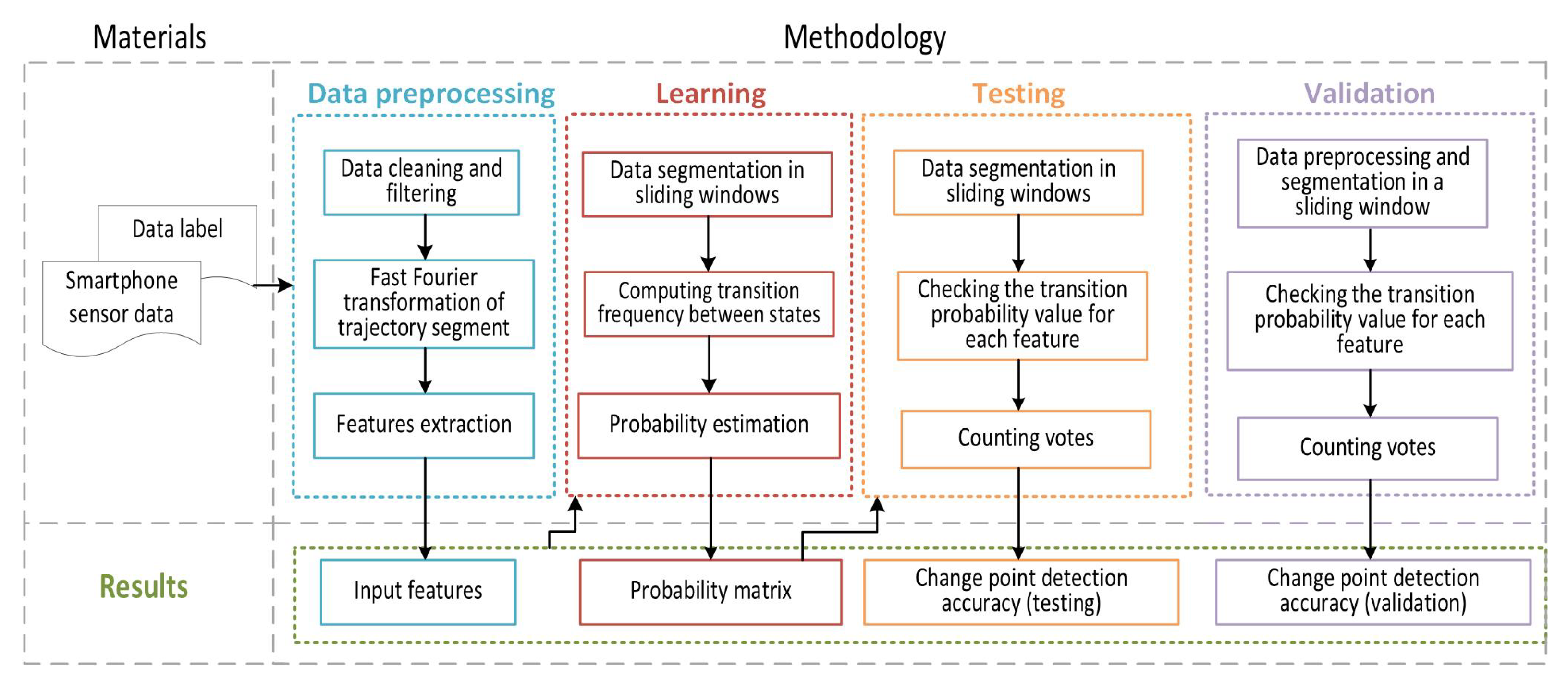
This section describes the methodology applied to develop the method for detecting MTPs in real time using TSM. The flowchart of the proposed approach is presented in Figure 1 and includes three parts: materials, a methodology for trajectory segmentation based on the transport mode criteria, and results. The methodology is divided into four parts:

(i)

data cleaning, filtering, transformation, and features extraction;

(ii)

dividing data into sliding windows, computing frequency and probability of transitions;

(iii)

checking transition probability for each time window in test data set and counting votes;

(iv)

checking transition probability for each time window in validation data set and counting votes.

3.1. Data Set

In this paper, we adopted benchmark The University of Sussex-Huawei Locomotion-Transportation (SHL) data set [39,40] usually used for multimodal transportation analytics [39]. SHL is a large-scale data set of smartphone sensor data recorded over a 7 month period in 2017. The data set contains 753 h of multimodal data: car (88 h), bus (107 h), train (115 h), subway (89 h), walk (127 h), run (21 h), bike (79 h), and still (127 h). Each user had a device in multiple places on the body to track the movement. The orientation of the mobile device is not necessarily fixed. The device’s location on the body is not important for this research, so the data collected with the device placed in the bag were taken. The data set contains data from seven sensors, but only data collected from a 3D accelerometer, gyroscope, magnetometer, and gravity were used in this study. Data are collected from all sensors with the frequency of 100 Hz. The training set contains $70\%$ of raw sensor data with appropriate labeling, whereas the test set includes $30\%$ of unlabeled data.

3.2. Data Preprocessing

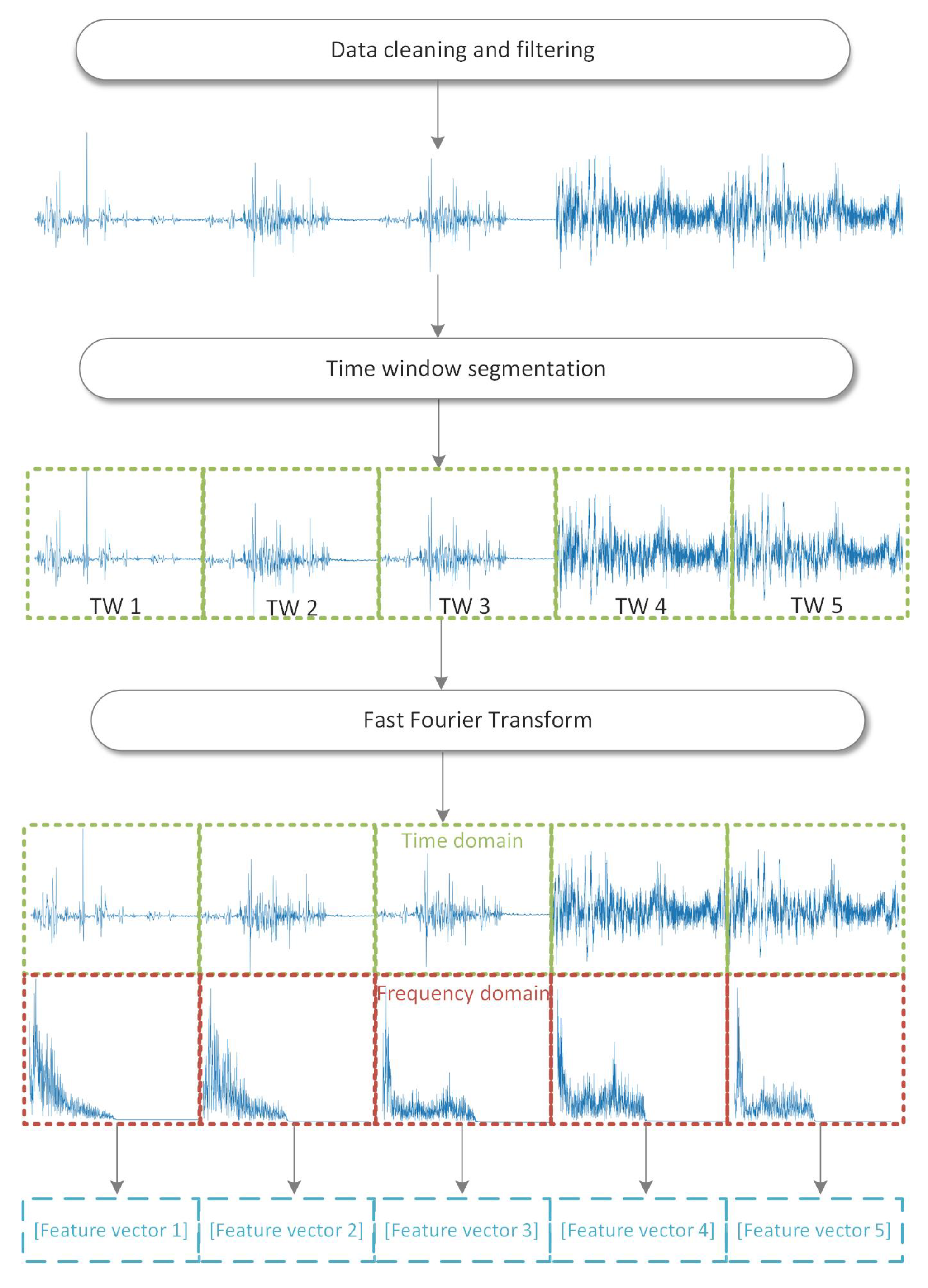
Data quality affects the data mining results, therefore before feature extraction, data need to be preprocessed. Data preprocessing steps are presented in Figure 2 where three main techniques for data preprocessing are presented:

(i)

data cleaning and filtering;

(ii)

time window segmentation;

(iii)

data transformation using Fast Fourier Transform (FFT).

Output parameters of each of the preprocessing steps are:

(i)

cleaned and filtered trajectory data;

(ii)

trajectory data segmented in time windows; and

(iii)

time and frequency domain data series in each time window.

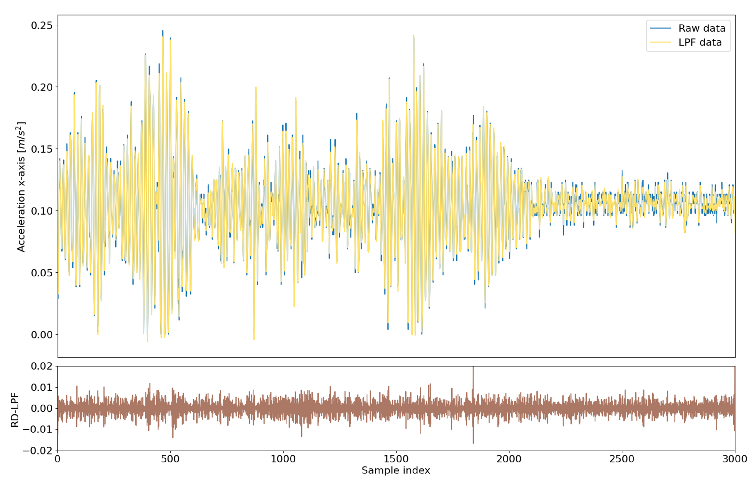
Raw signal data collected using mobile devices are highly affected by noise and missing values due to the signal degradation. Therefore, as shown in Figure 2, raw signal data should be cleaned and filtered. All records with missing values, as well as the unlabeled data, have been removed from the data set. For filtering of raw sensor data, a simple Low-Pass Filter (LPF) with a cut-off frequency of 25 Hz was applied [41,42,43]. A low-pass filter reduced the influence of sudden changes in the signal, so the filtered signal is smoother and less dependent on short changes. However, significant changes in the signal will not be removed by this filter, which is important in this research to retain the internal dynamic of the signal. Wang et al. [40] compared different subband features based on computed Mutal Information (MI) which indicates feature ability to distinguish target classes (transport modes included in SHL dataset). The highest MI values were observed for features in low frequency (below 25 Hz). Therefore, in this research, high-frequency data were removed.

In Figure 3, raw accelerometer data (blue line) and data filtered with LPF (yellow line) are shown. Parts of the data that represent periods when the signal has many spikes that often happen are removed from the LPF data. The difference between Raw Data (RD) and LPF data for each sample index (x-axis) is represented with the brown line. In addition, values given by the accelerometer are influenced by the acceleration of the body and gravity. An LPF separates these two components, resulting in values that reflect the more constant effects of gravity as the low-frequency component of the acceleration signal is mainly influenced by the gravity [42].

The next step is time window segmentation in order to simulate detection of the MTP in real time. First, data were divided into a time series of data points to ensure efficient real time detection of MTP. Window size is not uniformly agreed on in the trajectory segmentation research field, so the choice of the time window size is a contentious issue in the field. It is always a trade off between wide time windows which may include richer information about the activity but may increase misclassification when signals of two different transport modes fall into one time window. On the other hand, a short time window size improves tracking of fast transitions, but some essential patterns may not be captured [44]. A commonly used time window size in the human activity recognition field is 5 s, but 5 s is a too short period to observe the behavior during the transition from one transport mode to another because the time required for the transition is considerably greater. Akbari et al. [45] analyzed the influence of fixed time window sizes on the activity recognition using the SHL dataset. The influence of transition time from one transport mode to another is considered in time window size analyses. The authors tested different time window sizes: 15 s, 20 s, 30 s, and 1 min, and compared the F1 score of the classifiers.

The best score is achieved with the 30 s time window. Therefore, a non-overlapping 30 s sliding window to the trajectories in the training, testing, and validation data set is applied in this research. For example, Figure 2 shows that cleaned trajectory data after the time window segmentation step are divided into five non-overlapping time windows of the same size.

Data preprocessing ends with a data transformation step. Extracting discriminative features from the raw inertial data is essential, so many researchers are trying to describe the data better. In the field of mobile device sensor-based recognition, commonly, a transformation of raw signal data into a new data representation as a function of frequency and time is used [46,47]. In this research, data in one time window were transformed from the time domain to the frequency domain using the Discrete Fourier Transform (DFT) for discrete and periodic signals. Although the raw time data in one time window are not periodic, the commonly used workaround is to consider the whole time window data of the signal as the infinite periodic duplication of the actual time window data [48]. As the time window size is 30 s, and the sampling rate is 100 Hz, the considered period of the signal is 3000 samples. The DFT is computed using an FFT algorithm, commonly used for signals with more than 32 samples [48]. As shown in Figure 2, after applying FFT, each time window is represented with data in two domains: time domain and frequency domain (magnitude in polar notation).

Fundamental waveform characteristics of a given signal can be extracted from the time domain, while from the frequency domain, the structure of the signal can be extracted. More precisely, the magnitude represents the amplitude of cosine waves at a specific frequency. To make the interpretation more clear, an acceleration signal in one time window is considered. The time domain of the signal shows the amplitude of the signal, for example, showing if the person is accelerating suddenly (at the start of running), or at the slower pace (start of train movement). The frequency domain shows the spectrum of the signal. For example, if a person walks at the steady pace of 1 step in 1 s, as signal contains 3000 samples, there should be a spike in the frequency domain at 1 Hz (the $30/3000=0.01$ fraction of the sampling rate). The other example, for a car repeating its acceleration every 3 s, there should be a spike in the frequency domain at $0.33$ Hz (the $10/3000=0.0033$ fraction of the sampling rate). Therefore, if the frequency spectrum shows more high frequencies bandwidth, this means that the acceleration has changed frequently, and if it shows low frequencies bandwidth, the acceleration values have not changed so frequently.

3.3. Feature Extraction

The essential part before detecting MTP is to extract valuable and distinct information from time windows. Features are extracted in the time and frequency domain for each sensor. Furthermore, a challenging task in the raw signal data analysis is how to solve the orientation issue. In the SHL data set as well as in real life cases, smartphones can be carried in different orientations, meaning that the same sensor values in different cases can actually represent moving in different directions. Sensor orientation automatically changes data distribution and drifts, so it is difficult to distinguish whether a change in value occurred or a change in the orientation. Methods proposed in the literature often include heuristic transformation and singular value decomposition to transform the signal to another time-domain sequence in an orientation-invariant manner [49]. To overcome this constraint, computation of magnitude as $L2$-norm of $3D$ signal is often used [50,51,52]. In this paper, we computed the magnitude value for all sensors by Equation (1) where M is the magnitude, and $S_x$, $S_y$, and $S_z$ are sensor values along the x, y, and z axes, respectively. Due to the specificity of the magnitude calculation, it represents orientation-invariant feature.

$$M=\sqrt{S_x^2+S_y^2+S_z^2}$$

(1)

In summary, for every time window t, features are computed as a compound of the three axes’ (x, y, and z) sensor data with a magnitude vector. For each sensor, all features presented in

Table 1. List of features in time and frequency domain.

Feature	Time Domain	Frequency Domain	Description
Mean	✓	✓	Average value.
Variance	✓	×	Spread between numbers.
Standard deviation	✓	×	Dispersion of data set relative to its mean value.
Median	×	✓	Middle of the sorted list of numbers.
Skewness	✓	×	Measure of symmetry.
Kurtosis	✓	×	Measure of relative peakedness of a distribution.
Z score	✓	×	Indicates how many standard deviations an element is from the mean value.
Interquartile range	✓	×	The difference between the 75th and 25th percentiles of data.
Peak to peak	✓	×	The difference between the maximum and the minimum amplitudes of data.

are computed. Combining all sensors with their features are input parameters to the algorithm.

As shown in Table 1, commonly used statistical features such as mean, variance, standard deviation, median, kurtosis, and skewness were extracted for the time or frequency domain. In many research, it has been highlighted that statistical features play an essential role in the area of sensor-based recognition [53,54,55]. The skewness of data in time window indicates a symmetrical or asymmetrical distribution of data, while kurtosis describes data distribution.

Feature z score shows the distance of the data in the current time window to the mean value. Distance is measured in the standard deviations, and the total score is computed by Equation (2), where $Y_t$ is the mean value of the data in the current time window, and $\mu$ and $\sigma$ are mean and standard deviation of all data obtained up to that time window. These two values are computed cumulatively until a change point is detected between the two time windows, at which point both values are reset to zero.

$$z=(Y_t-\mu )/\sigma$$

(2)

Interquartile range and peak to peak features are used as measures of the spread of the data. The InterQuartile Range (IQR) measures the spread of the middle half of the data, and it is computed by Equation (3) where $Q_3$ represents the third and $Q_1$ the first quartile of the data.

$$IQR=Q_3-Q_1$$

(3)

Feature Peak To Peak (PTP) measures the difference between the minimum and maximum value of data in one time window, and it is computed by Equation (4) where $MAX$ represents the maximum and $MIN$ the minimum value of time window data.

$$PTP=MAX-MIN$$

(4)

3.4. Transition State Matrices

Many methods have been introduced to find change points in time series. To detect change point in each subsequence or time point, the constructed model has to accurately predict a time window label based on the past feature values. Hidden Markov Model (HMM) is one of the most popular models in the literature for sequential data processing as it does not suffer from labor-intensive computations and can model the dynamic behavior of time series with a simple variable model [9,56,57]. Additionally, probabilistic models are also more robust to noise.

Considering the reasons mentioned above, we adapted the HMM to form TSM to detect MTP. A TSM is a matrix that describes transitions between two consecutive time windows, t and $t+1$, using feature values. The extracted features are the input data for the TSM. Each feature between two consecutive time windows is described with two matrices: no change transition state matrix and change transition state matrix. All transitions between consecutive time windows with no change in the transport mode are recorded in the no change matrix. Change matrices were created in the same way but referring only to transitions in which change of transport mode occurred.

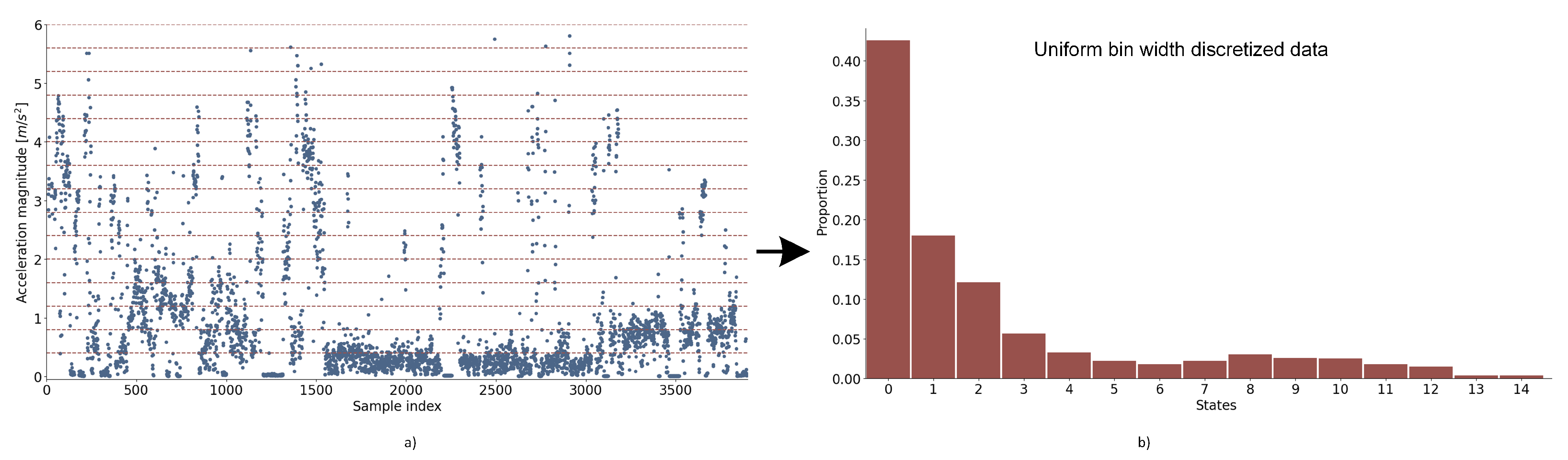
The equal width discretization procedure converts continuous feature data to discrete states. Figure 4a shows an example of discretization procedure for mean acceleration magnitude values (y-axis). On the x-axis are sample indexes in the training dataset. The range of data (i.e., the difference between the minimum and maximum observed value) is divided into 15 equal-width bins (red dashed lines). Each bin represents one state in the TSM. The result of discretization is shown in Figure 4b, where data distribution between states is shown. The number of data points in each state is divided by the total number of data points. Uniform width bins preserve general data distribution but produce some bins with low probabilities, for example, states 13 and 14. The equal width discretization procedure is repeated for each feature and sensor value combination.

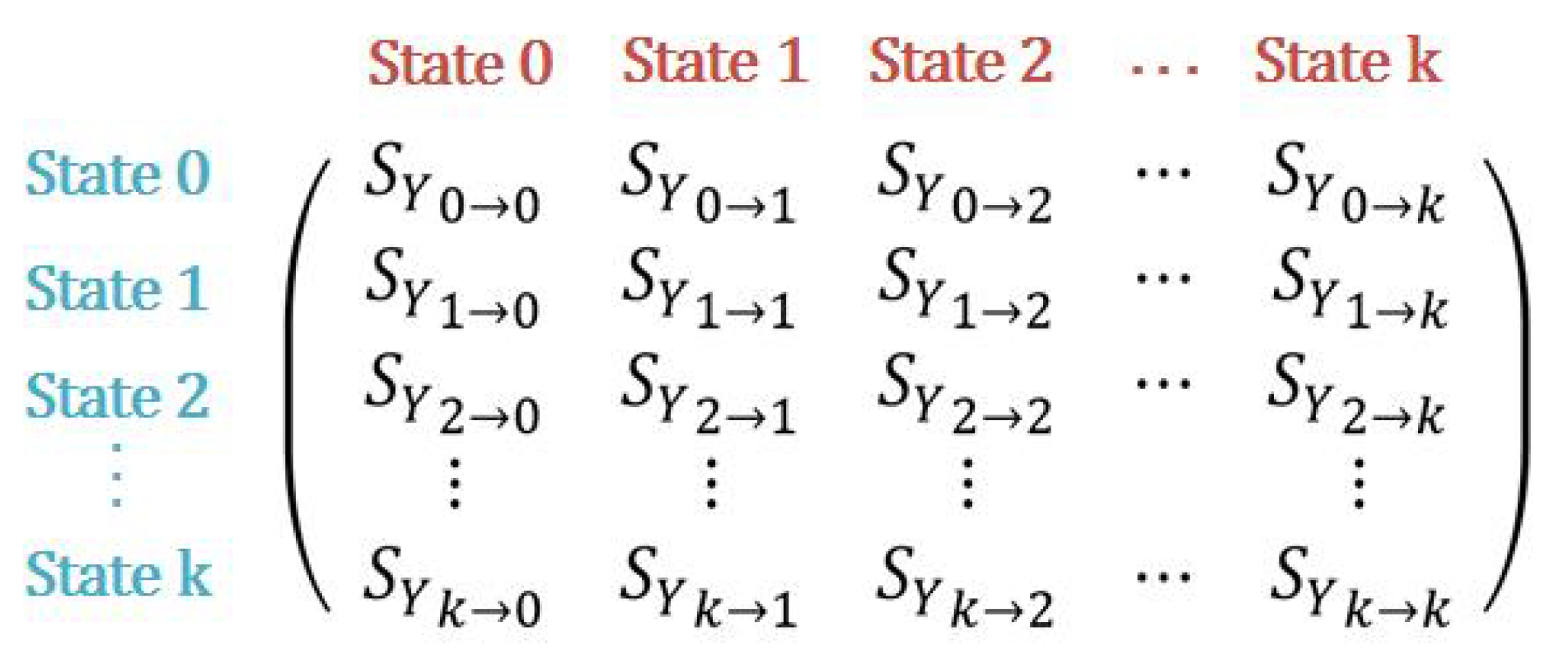
As shown in Figure 5, each matrix consists of k rows and k columns. The columns and rows breakpoints are states obtained by equal width discretization. This means that each feature has 15 states, and each value of the feature vector of the current (streaming) time window will belong to exactly one state of the feature. As a result, the TSM has $15\times 15=225$ transitions between feature states. The transition represents the transition between two states of two consecutive time windows for the observed feature. Then, for each transition, it is counted how many times such a transition is noted as a change or no change in the transport mode. For instance, for transition $Y_{0\to 1}$, it is counted how many times, $S_{Y_{0\to 1}}$, time window t goes from state 0 to state 1 in time window $t+1$ for the observed feature. This is observed for transitions in which changes and no changes between transport modes occurred. The result of this procedure are two matrices (change and no change) of transitions that represent the frequency of each transition occurrence.

In order to use such matrix for prediction, it is necessary to compute the probability of a change in the transport mode for each transition. The probability was computed for each transition using Equation (5) where $S_{Y_{i\to j}}$ is the number of occurrences of transport mode with change events during transition from state i to state j, and in the denominator is the sum of all matrix elements.

$$P_{ij}=\frac{S_{Y_{i\to j}}}{{\sum }_{i=0}^k{\sum }_{j=0}^k{S}_{Y_{i\to j}}}$$

(5)

In probability matrices for transitions when there was no change in the transport mode, $S_{Y_{i\to j}}$ represents the number of occurrences of transport mode with no change events. Using the TSM, the observed outputs are predicted in the testing phase, and the voting procedure is described in the Section 3.5.

3.5. Testing

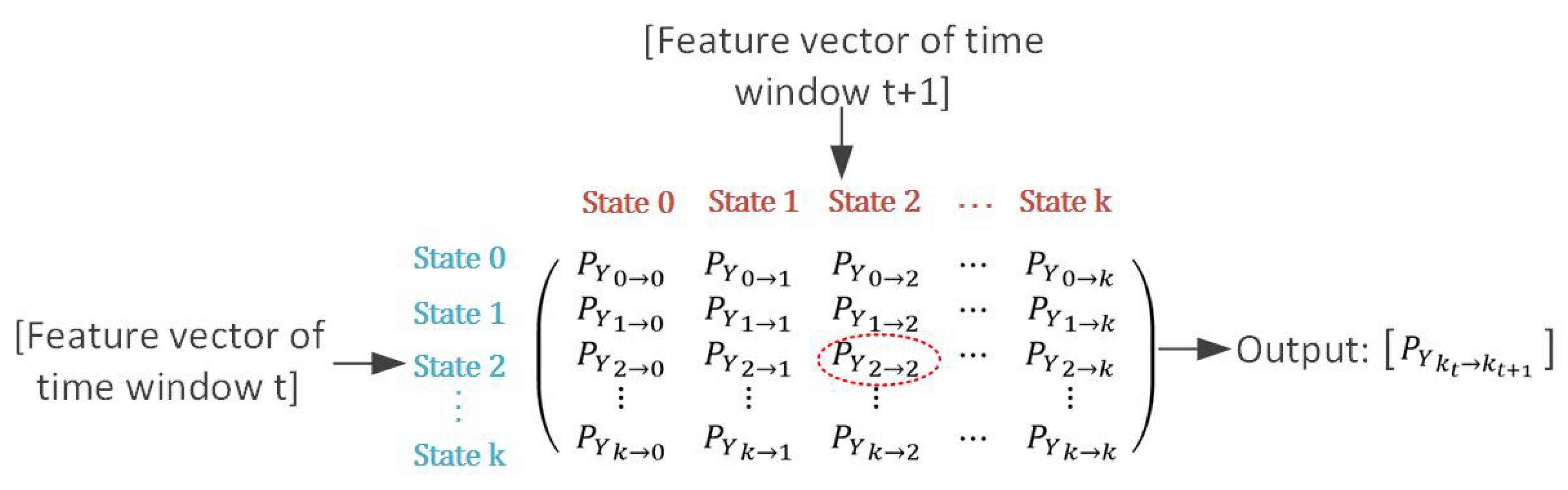
In the prediction process, for each transition between two consecutive time windows, 160 matrices are computed (4 sensors × (3 axes + $L2$-norm)) × 10 features = 160 matrices) for each class. Accordingly, for each transition, there are 160 pairs of probability values. As shown in Figure 6, the probability of each transition is determined by two feature vectors, the feature vector of the time window t and consecutive time window $t+1$. A value in feature vector for time window t represents a corresponding row in the TSM, while the value in feature vector for time window $t+1$ represents a corresponding column. One element of TSM (red dashed elipse in Figure 6) represents the probability that a change or no change (depending on the observed matrix) has occurred between time window t and time window $t+1$. If the probability for change in TSM change matrix is higher than no change probability in TSM matrix for no change, then this feature gives a vote for a transport mode change, otherwise gives a vote for no change. The procedure is repeated for feature values in feature vector t and feature vector $t+1$. In the end, the output label (change or no change) that received more votes from all features is selected.

At this stage, the model’s accuracy was computed based on comparing the actual and the predicted value. However, additional measures have been introduced to assess the accuracy due to the specific characteristics of the problem. Namely, each trajectory contains a large number of transitions between time windows in which there was no change in the transport mode and a small number of transitions in which there was a change in the transport mode. For example, a route that lasts 80 min where the user changed three transport modes during the route has only two time windows in which a change of transport mode occurred, and in the remaining 158 time windows, there was no change. Thus, the overall accuracy can be high without detecting the time windows in which the change actually occurred. Therefore, for method evaluation, a confusion matrix with all performance metrics is highlighted as a more relevant measure of comparison.

3.6. Validation

The data set used to validate the proposed methodology for MTP detection was collected on the transport network in Croatia. The main difference between validation and SHL data set is the location, and therefore the different traffic network, on which the data were collected. Android application Collecty, developed in the Android Studio, was used to collect the data set. The application continuously runs in the background and collects data from mobile device sensors. Five subjects had their mobile device with application turned on during the collection. For this type of research, the emphasis is not on the structure or number of subjects, but rather on the accuracy and quantity of collected data in hours. These parameters in the validation data set are comparable to the state of the art SHL data set. The subject could select one of the eight transport modes: car, bus, train, bike, tramway, walk, run, and e-scooter.

Figure 7 briefly shows the application and its functionalities. After registration, the user chooses which transport mode is currently used. When changing the transport mode, the user changes the current transport mode by pressing the $ChangeMode$ button. At that point, the transport mode of all further records is changed until the user changes the transport mode again or completes the route. The user signals the end of the route by pressing the $EndRoute$ button, after which an entire route is displayed using Open Street Map. Parts of the route with different transport modes are represented with different icons, ensuring data validation. When user confirms the displayed route, data are permanently written to the database.

After collecting the data, the same process as in model testing was applied to obtain the validation results.

4. Results

This section presents testing and validation results obtained by the complete and reduced feature sets. The results are organized into three subsections:

(i)

TSM analysis;

(ii)

testing;

(iii)

validation results.

4.1. Transition State Matrices Analysis

The entire data set is marked with seven different transport modes and one user state, which are not the primary labels of this research. Therefore, the data set is customized on two data labels: change (time window in which change in the transport mode occurred) and no change (time window in which there was no change in the transport mode).

The training sample contains 3900 instances, while the testing set contains 1700 instances for each axis of each sensor data. There are 107 transitions from one transport mode to another in the training data set and 21 such transitions in the test data set.

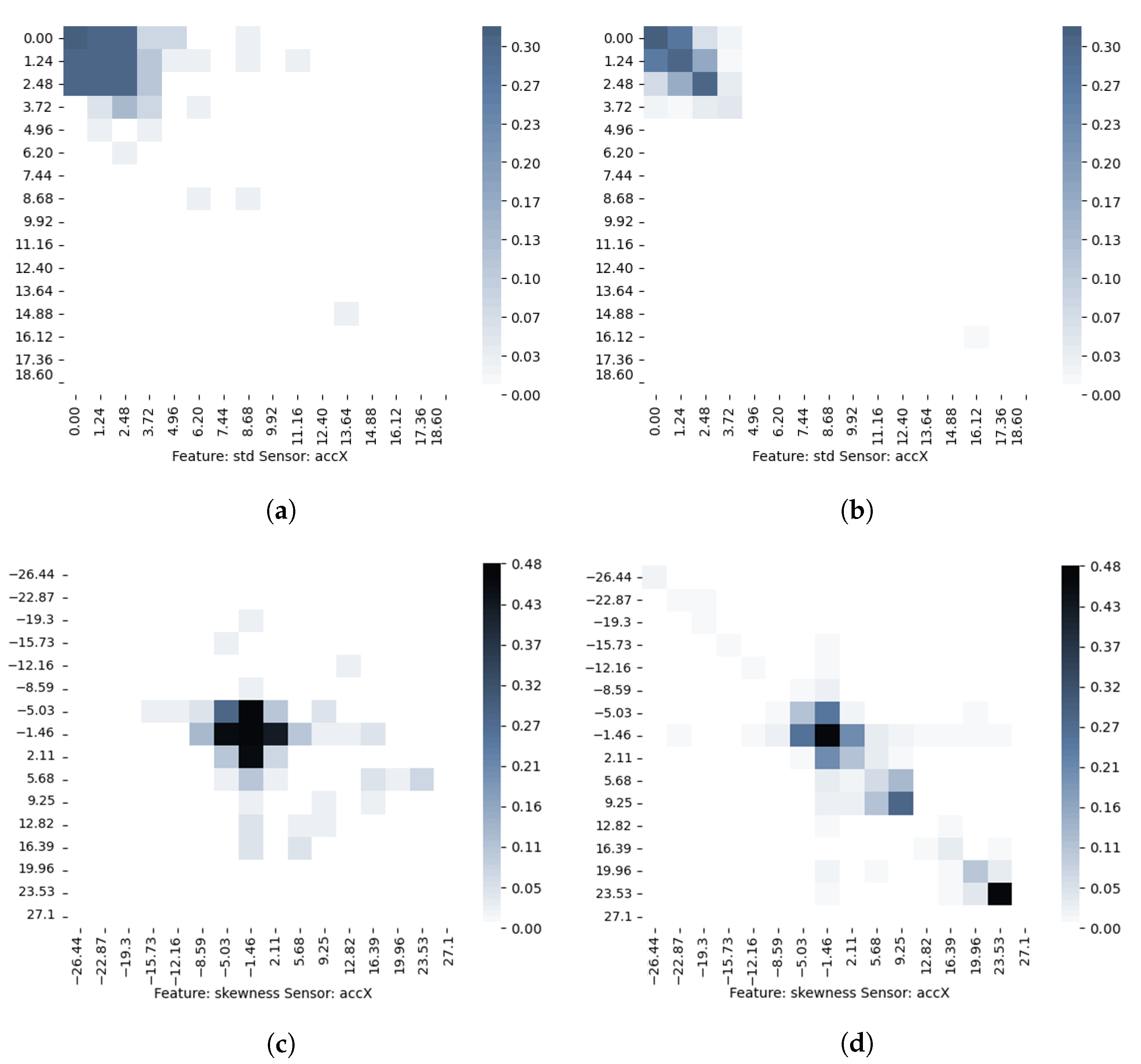
After training the model, the number of TSMs is doubled because each TSM was created for change and no change class. Along x and y-axis of the TSMs in Figure 8 are the values of the corresponding TSM feature divided into 15 states. The color intensity from white to dark blue indicates the probability of transition between states. Figure 8a,b represents TSMs for the standard deviation feature and the acceleration sensor along the x-axis, and Figure 8c,d are TSMs for the skewness feature and the acceleration sensor along the x-axis. In the left column, TSMs for time windows in which there was no change in the transport mode are presented, and in the right column, TSMs for time windows in which there was a change in the transport mode are presented. In Figure 8a,b the most frequent transitions between states are mostly the same. However, there is a greater scattering of different states in the matrix for transitions with no change. On the contrary to this pair of matrices, matrices in Figure 8c,d show a shift in the most common states for the transport mode change and no change classes.

4.2. Testing Results

To evaluate the performance of the proposed MTP detection framework, we computed four performance metrics: accuracy, recall, precision, and specificity. Predicted values were compared with ground truth labels in the current and five adjacent time windows. A comparison of label values in adjacent time windows was introduced because it was observed that the model detects a change of transport mode in the time window in which the change in the transport mode occurred and in the adjacent time windows. This can be explained by the short duration of the time window while the most common duration of changing the transport mode is longer than 30 s. Therefore the change of transport mode is reflected in the neighboring time windows.

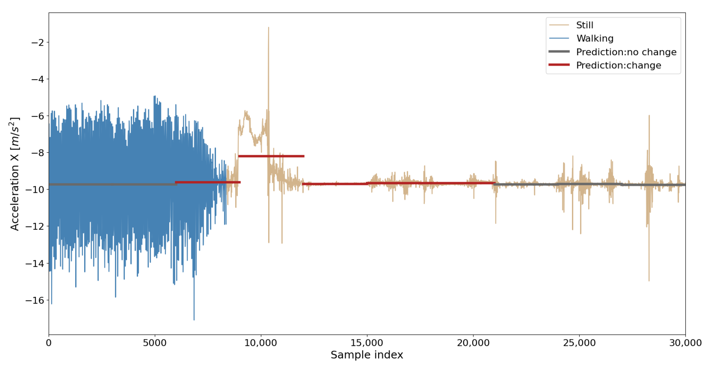
For example, Figure 9 shows the raw x-axis acceleration values on y-axis and time samples on x-axis, whereby in the 8372nd time sample, a change in the transport mode occurred (change in the color of the curve in the figure). The centerline represents the mean value of the acceleration along the x-axis in observed time windows. Centerline color indicates whether the time window is classified as a time window in which change of transport mode occurred (red) or not (gray). In this case, it is evident that a change in the transport mode is predicted in the correct time window, but a change is also predicted in the following few time windows. Change that occurred at one point in time affected feature values in the adjacent windows as well, which causes false positive predictions for those time windows. However, such cases cannot be considered as prediction errors because they relate to a change in transport mode that occurred in past $2.5$ min, and this time is sometimes referred to as the time required for a user to physically switch from one transport mode to another [58]. Therefore, in this paper, the prediction is considered correct if the change of transport mode is detected within 3 min from the moment of the actual transport mode change.

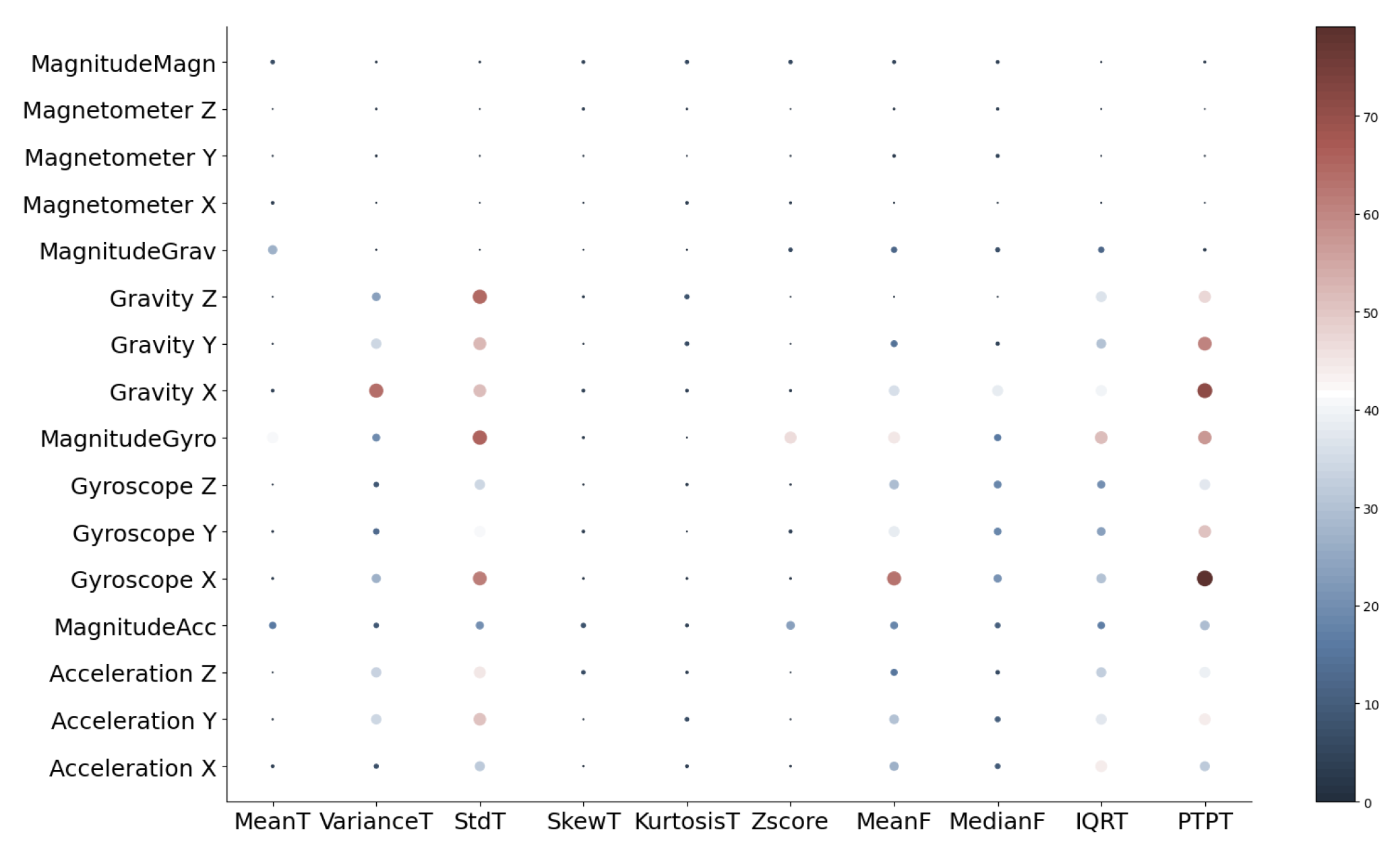
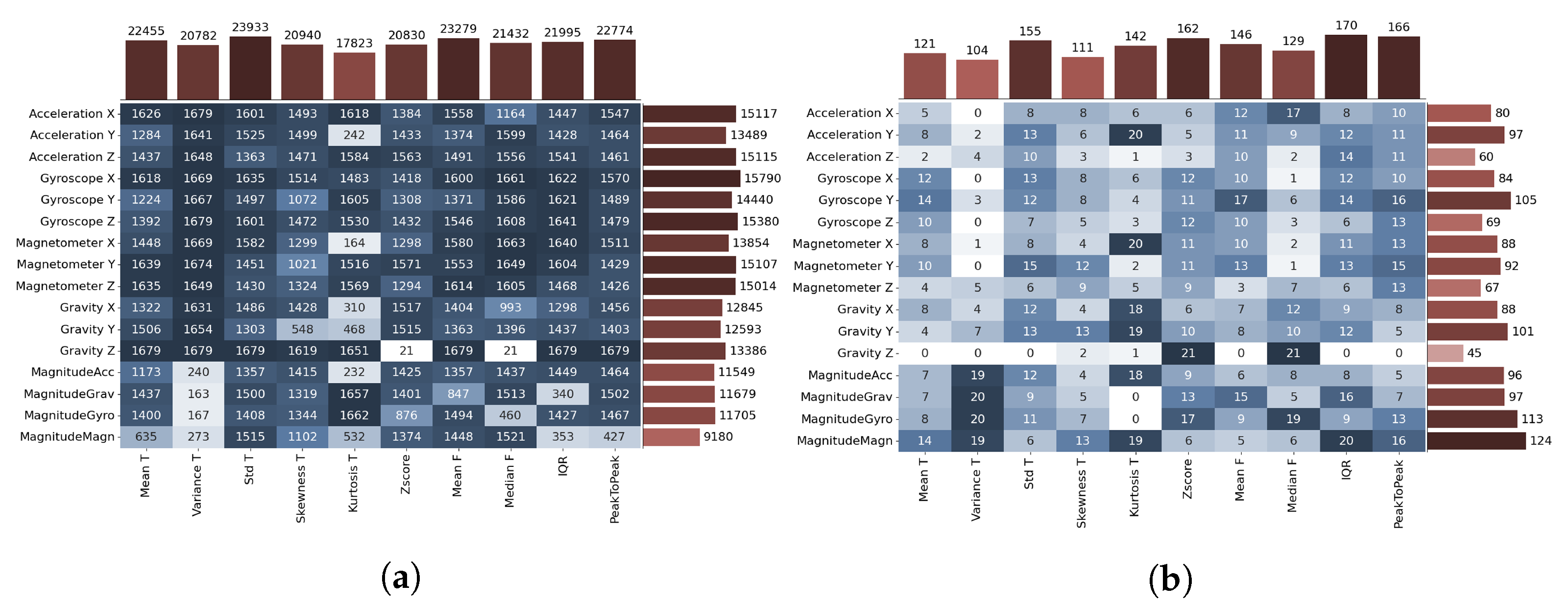
The impact of each feature and sensor on the prediction result was observed in order to find meaningful features that better describe original data. Figure 10 shows two matrices showing how many times each feature (x-axis)- sensor (y-axis) combination has given an accurate prediction for all time windows in the data set, Figure 10a, and for time windows in which the change of transport mode occurred, Figure 10b. The letters T and F next to the feature name indicate the time and frequency domain. Light to dark color gradient indicates less to more accurate features. Bins at the top of the graph show the distribution of the feature (column) total correct predictions, and bins placed on the right of the graph show the distribution of the sensor (row) total correct predictions. In the matrix with all time windows, it can be seen that the measures standard deviation in the time domain and mean in the frequency domain have the highest frequency of accurate prediction, and the gyroscope along the x and z-axis is in the lead of all sensors. On the contrary, the variance and kurtosis show the worst prediction result.

Initially, this analysis was performed to improve model accuracy using features that showed promising results in the model prediction. A separate analysis of feature predictions for time windows where a change of the transport mode occurs is important due to the lower number of samples with the actual change of the transport mode. In Figure 10b, it can be seen that features with the worst prediction score in the entire data set, such as kurtosis, are showing better results when only a subset of data, where change occurred, is observed.

A reduced feature data set is obtained using univariate feature selection. First, features whose false positive rate test score is significant are excluded from the feature set, and secondly, features are sorted according to the highest ANOVA F score. Thus, we determined which features give the most information about the data and which features are uncertain. Figure 11 shows a feature importance which is represented as filled circles with two attributes:

(i)

size, which represents the importance of feature; the greater the importance is, larger the circle is;

(ii)

color, from dark blue to dark red, represents F score value.

The y-axis represents sensors, and the x-axis represents features. The best F score is achieved for the feature peak to peak and sensor gyroscope along x-axis. Therefore, arranged features were the input for testing the model accuracy with different number of features.

Accuracy, recall, and F1 score are used to validate the model performance. Accuracy is the proportion of the correct predictions, and the F1 score is a weighted average of the recall and precision (correctness achieved in positive prediction). The influence of the F1 score on the model performance is significant because it shows the balance between the prediction of true negatives and true positives. However, a recall has been added due to the specificity of the problem in which the emphasis is on accurately predicting change. A recall measures positive examples which are labeled as positive by the classifier (changes classified as changes). The main disadvantage of the model with all features is that it was overfitted to a no change class due to a higher number of samples of such class in the training data set. Therefore, the optimal ratio of these three measures was considered to select the number of features in the reduced-feature model, which is in the end set to 45.

The confusion matrix is presented in

Table 2. Confusion matrix for testing results.

	Full-Feature Model		Reduced-Feature Model
	Predicted Change	Predicted Nochange	Predicted Change	Predicted Nochange
Actual change	14	7	17	4
Actual nochange	15	1664	21	1658
Accuracy	98.7%		98.52%
Recall	66.67%		80.95%
Specificity	99.1%		98.75%

for the method with all and reduced number of features. Due to the imbalance between the number of changes and no changes in trajectories, three main performance metrics are used to validate the performance of the proposed method. From Table 2, when all features are used, the proposed method achieved accuracy, recall, and specificity of $98.7\%$, $66.67\%$, and $99.1\%$, respectively. Recall results are better for the reduced-feature model, resulting in the value of $80.95\%$.

The observed value for precision is $48.28\%$, which is considerably lower than achieved values for other performance metrics. Precision represents the ratio of the total number of correctly classified positive examples and the total number of predicted positive examples. In applications such as detection of change point, it is quite common to have imbalanced class distributions, as there are far fewer time windows where a change of transport mode occurred than the time windows with no change. Therefore, precision will be lower due to the larger number of samples with no change in transport mode. This is why it is necessary in such cases to balance between precision and recall. In MTP detection, it is better to false detect the MTP than not to detect the MTP at all. For this reason, the emphasis in this problem is on the recall and not on the precision.

4.3. Validation Results

To validate the proposed model, our own data set was collected. A total of 38 multimodal routes containing 71 transitions between transport modes and 3425 time windows (30 s) were collected. Only those transport modes specified in the SHL data set were used in all routes.

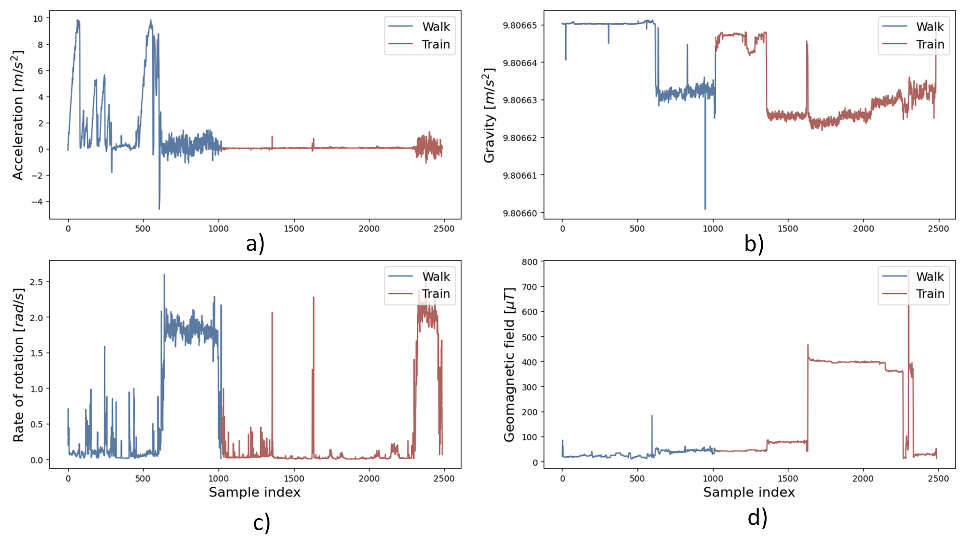
Figure 12 shows an example of raw sensor data (y-axis) in time samples (x-axis) in validation data set in which two connected transport modes were used: walking and train with one change point (change in the color of the curve in the figure). In trajectory, four mobile device sensors were monitored and used for model validation.

Magnitude of acceleration and magnitude of geomagnetic field (Figure 12a,d) show different values when using different transport modes while the magnitude of gravity and magnitude of rate of rotation (Figure 12b,c) do not show obvious differences in raw data when using different transport modes.

Table 3. Confusion matrix for validation results.

	Predicted Nochange	Predicted Change
Actual nochange	3239	115
Actual change	14	57
Accuracy	96.23%
Recall	80.28%
Specificity	96.57%

shows the confusion matrix for validation results conducted with reduced-feature model. Validation results show that the model’s accuracy is close to the test results, so it can be concluded that the model is stable. The total achieved accuracy of the model is $98.52\%$ in the testing phase and $96.23\%$ in the validation phase, which is a difference of $2.3\%$. The recall difference between the testing and validation phase is less than $1\%$.

Validation results are similar to the test results and confirm that the different geographical location, i.e., different transport networks on which the data are collected, does not affect the method’s accuracy. Namely, the data for training and testing of the method are part of the SHL data set, while the data for validation are collected on the transport network of Croatia. These are two completely dislocated (different countries) and different transport networks. Thus, comparable validation and test results confirm the assumption of the geographical independence of the implemented method.

5. Conclusions

In this paper, a method for trajectory segmentation in real time based on the transport mode change criterion using TSM was developed. Trajectory segmentation was performed on data collected from mobile device sensors. The data were described by features in the time and frequency domain. FFT was used to convert data from time domain to frequency domain. In total, 10 statistical measures, 12 different types of sensor measurements, and $L2$ norm for each sensor type were used to train the model, resulting in 160 matrices for each label value (change or no change). After testing, the used features were analyzed, and the number of features was reduced. The results of both models were presented: with all features and the reduced number of features with a best overall accuracy of $98.52\%$ and recall value of $80.95\%$. The proposed method demonstrates the validity of the TSM to enhance transport mode trajectory segmentation and to enable real time detection of MTP.

To validate the model in real time, we collected our own data set. Data are collected using the Android application Collecty which is briefly presented in the paper. The collected data set contains 38 routes in which at least two different transport modes are used. After validation, an overall accuracy of $96.23\%$ and a recall value of $80.28\%$ were achieved. Results confirm the assumption that the method does not lose accuracy when applied to data set collected in areas with different transport mobility patterns. Although we have achieved high performance results by TSMs, there is a space for improving the proposed MTP detection framework. The TSM model will perform better with a higher amount of data, particularly a higher amount of data in which the change occurred. Therefore, as a future research direction, TSM can be supplemented with additional data or through the online learning process to achieve better model accuracy.