Article

A Simulation-Optimization Modeling Approach for Conjunctive Water Use Management in a Semi-Arid Region of Iran

1
Department of Geology, Payame Noor University (PNU), Tehran 193954697, Iran
2
Department of Water Engineering, Aburaihan Campus, University of Tehran, Tehran 3391653755, Iran
3
Department of Water Engineering, Faculty of Agriculture, University of Tabriz, Tabriz 5166616471, Iran
4
Warnell School of Forestry and Natural Resources, University of Georgia, Athens, GA 30602, USA
5
Department of Water Science and Engineering, Islamic Azad University, Science and Research Branch, Tehran 1477893855, Iran
6
Research Institute of Forests and Rangelands, Agricultural Research, Education and Extension Organization (AREEO), Tehran 1496813111, Iran
*
Authors to whom correspondence should be addressed.
Sustainability 2022, 14(5), 2691; https://doi.org/10.3390/su14052691
Submission received: 2 February 2022 / Revised: 22 February 2022 / Accepted: 23 February 2022 / Published: 25 February 2022
(This article belongs to the Section Sustainable Forestry)

Abstract

:
Agricultural months are the critical period for the allocation of surface water and groundwater resources due to the increased demands on water supplies and decreased recharge rate. This situation urges the necessity of using conjunctive water management to fulfill the entire water demand. Here, we proposed an approach for aquifer stabilization and meeting the maximum water demand based on the available surface and groundwater resources and their limitations. In this approach, we first used the MODFLOW model to simulate the groundwater level to control the optimal withdrawal and the resulting drop. We next used a whale optimization algorithm (WOA) to develop an optimized model for the planning of conjunctive use to minimize the monthly water shortage. In the final step, we incorporated the results of the optimized conjunctive model and the available field data into the least squares-support vector machine (LS-SVM) model to predict the amounts of water shortage for each month, particularly for the agricultural months. The results showed that during the period from 2005 to 2020, the most water shortage belonged to 2018, in which only about 52% of water demand was met with the contribution of groundwater (67%) and surface water (33%). However, the groundwater level could have increased by about 0.7 m during the study period by implementing the optimized model. The results of the third part revealed that LS-SVM could predict the water shortage with better performance with a root-mean-square error (RMSE), mean absolute percentage error (MAPE), and Nash–Sutcliffe Index of 5.70 m, 3.43%, and 0.89 m, respectively. The findings of this study will enable managers to predict the water shortage in future periods to make more informed decisions for water resource allocation.

1. Introduction

Due to the scarcity of water supplies in many regions worldwide, and the potential changes in rainfall trends due to climate change [1,2,3], water withdrawal and consumption should be carefully managed. Given society’s desire to develop products that are in demand and to provide maximum profit, water supplies have diminished at an alarming rate [4,5]. The loss of freshwater and groundwater resources, depletion of aquifers, water stress and scarcity, land degradation, and desertification are some of the consequences of inappropriate water management around much of the world [6,7]. The 2018 edition of the United Nations World Water Development Report of 2018 stated that nearly 1.8 billion people will be living in regions that experience absolute water scarcity by 2050. The projection also suggests that water scarcity will displace about 24–700 million people worldwide by 2030. On the other hand, the demand for agricultural production is projected to increase by about 50% in 2050 [8]. To address these crises, researchers and managers are working together to adopt efficient management strategies for handling current and future challenges [9].
Conjunctive use of water resources is a strategy that connects, combines, and harmonizes the use of surface water and groundwater in order to maintain balance within the water demand/supply system. The first research on conjunctive water use dates back to eighty years ago [10]. Over time, many studies and advances in this field have been performed [11]. Several researchers have recently investigated the conjunctive use of water resources to inform strategies for water management in regions of the world that suffer from water scarcity [12,13,14]. By examining the implications of restrictions on the exploitation of surface and groundwater resources, this conjunctive use analysis enables land managers to not only maximize or satisfy water demand but also ensure that water resources are managed sustainably [15]. Conjunctive use of water resources has received attention in almost every part of the world, especially India [16], Iran [13], China [17], and the USA [18], where water managers have acknowledged that conjunctive use may be a component of solutions that focus on the problems of allocating reclaimed water, surface water, and groundwater to different water users over different months of the year. This type of approach to water planning focuses on aquifer balancing, water quality protection, reservoir shortage protection, groundwater level maintenance, and water right determination [19] for meeting society’s needs [20,21]. While they often focus on water-deprived regions of the world, conjunctive use analyses can also be applied in water-rich regions to inform land managers about options for slowing groundwater level rises and minimizing water deficits. These benefits of conducting conjunctive use analyses are of great importance given the increasing water demand from a world population approaching eight billion people.
Optimal conjunctive use management heavily relies on simulation and optimization processes where objectives are adjusted with respect to the constraints of every specific region [6]. Some researchers [22,23,24] have used conjunctive models of optimization simulators with MODFLOW code and different optimization scenarios to manage the conjunctive groundwater use. Optimal conjunctive use plans have been developed with numerical modeling of groundwater and nonlinear optimization algorithms [25,26]. The evolutionary optimization algorithms that have been suggested and applied to the problem of conjunctive use include genetic algorithms [12,13,17], nondominated sorting genetic algorithm [27], ant colony optimization [24], particle swarm optimization [28], genetic programming [29], dual fitness particle swarm optimization [30], extreme-point-based multi-objective particle swarm optimization [31], gravitational search algorithms [14,32], and Jaya algorithm optimization [33]. These are all considered to be p-metaheuristic combinatorial optimization processes where a population of feasible (usually) solutions is modified through various means to direct the entire set, and a single solution in particular, toward the optimal solution. These processes, while able to produce high-quality solutions to combinatorial problems, do not guarantee optimality, however. Further, the examples of numerical methods that have been applied to the conjunctive use problem include groundwater vistas [34], the soil water atmosphere plant (SWAP) model [35], Bayesian networks [36], linear programming [37], nonlinear programming [38], hydrogeological and agronomic models [39], mixed-integer nonlinear programming [40], and MODFLOW and fuzzy inference systems [41].
Depending on how these algorithms were implemented, they may be efficient in solving conjunctive use problems. However, researchers recommend extending the exploration of potential tools to a broader range of methods/algorithms in an effort to improve the accuracy and reliability of outcomes [42,43,44]. Recently, research has been conducted on using intelligent models for optimal conjunctive use. This method is a completed version of the simulation/optimization technique. In this approach, the results of the optimization model are trained by an intelligent model, and the trained model can be utilized instead of the optimization simulation model [41]. The developed model can be used for any time and climatic conditions; in addition, it is not time-consuming and difficult, in contrast with simulation/optimization techniques.
Machine learning models have gathered considerable attention due to not requiring the physical information of the channels and their physical structure [45,46,47]. LS-SVM models have also been used in various studies, including longitudinal dispersion coefficient prediction, predicting monthly evaporation from dam reservoirs, predicting groundwater storage loss, and sensor development showing a great performance [48,49,50].
In the present study, we illustrate the development of a simulation-optimization modeling approach that combines MODFLOW code, the Whale Optimization Algorithm (WOA), and least squares-support vector machine (LS-SVM) processes to address the conjunctive water use planning problem in a semi-arid region (Marvdasht) of Iran. The following objectives guide this study: (i) develop a conjunctive use approach for sustainable use of surface and groundwater resources that will produce near-optimal solutions; (ii) illustrate how water demands can be maximized based on the potential of surface water and groundwater; (iii) evaluate the efficiency of the WOA in providing near-optimal outcomes for allocating surface water and groundwater; (iv) develop an intelligent model that can predict monthly water shortages, especially for agricultural months; and (v) evaluate the efficiency of LS-SVM for assisting in the prediction of monthly water shortages.

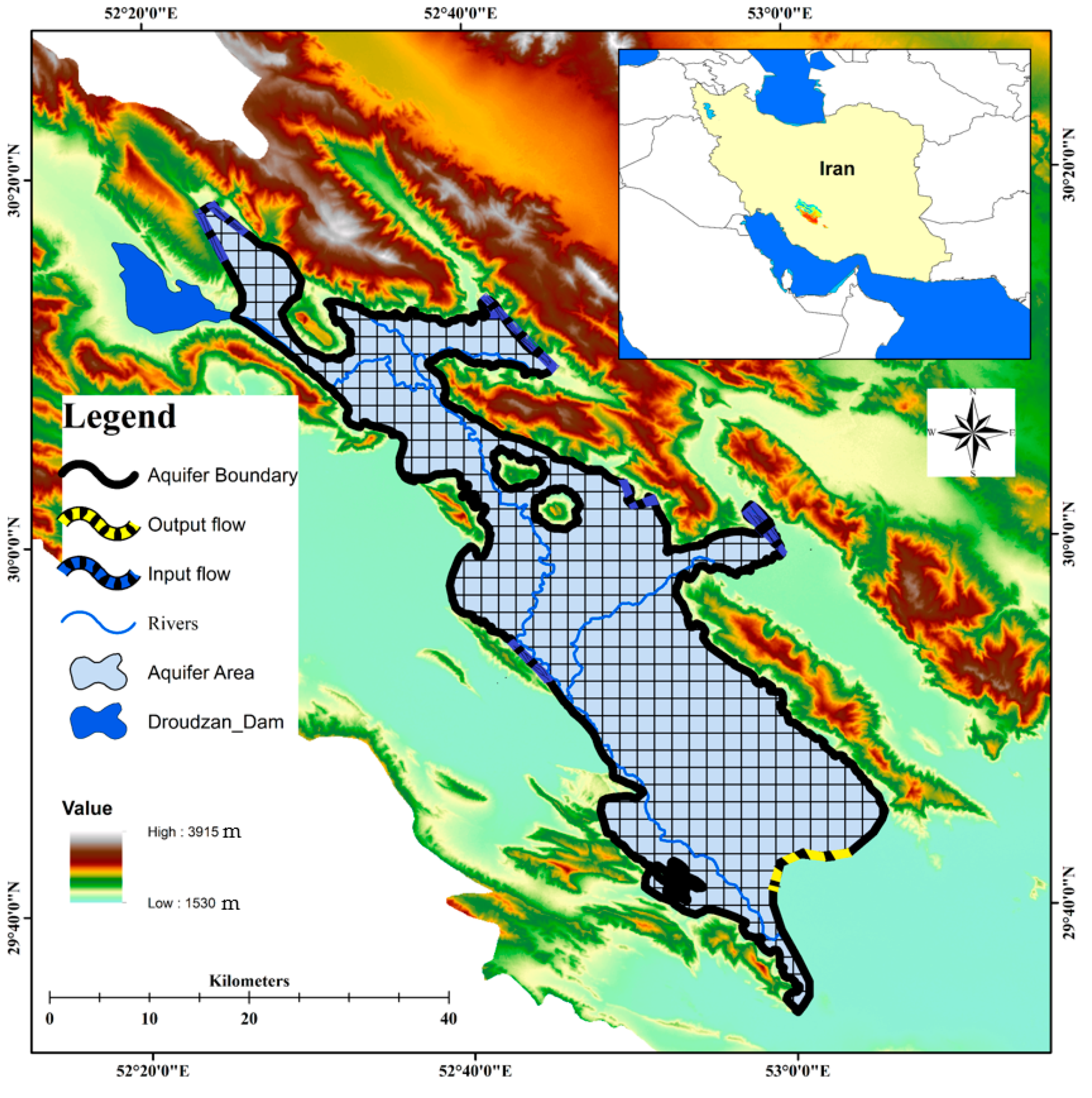
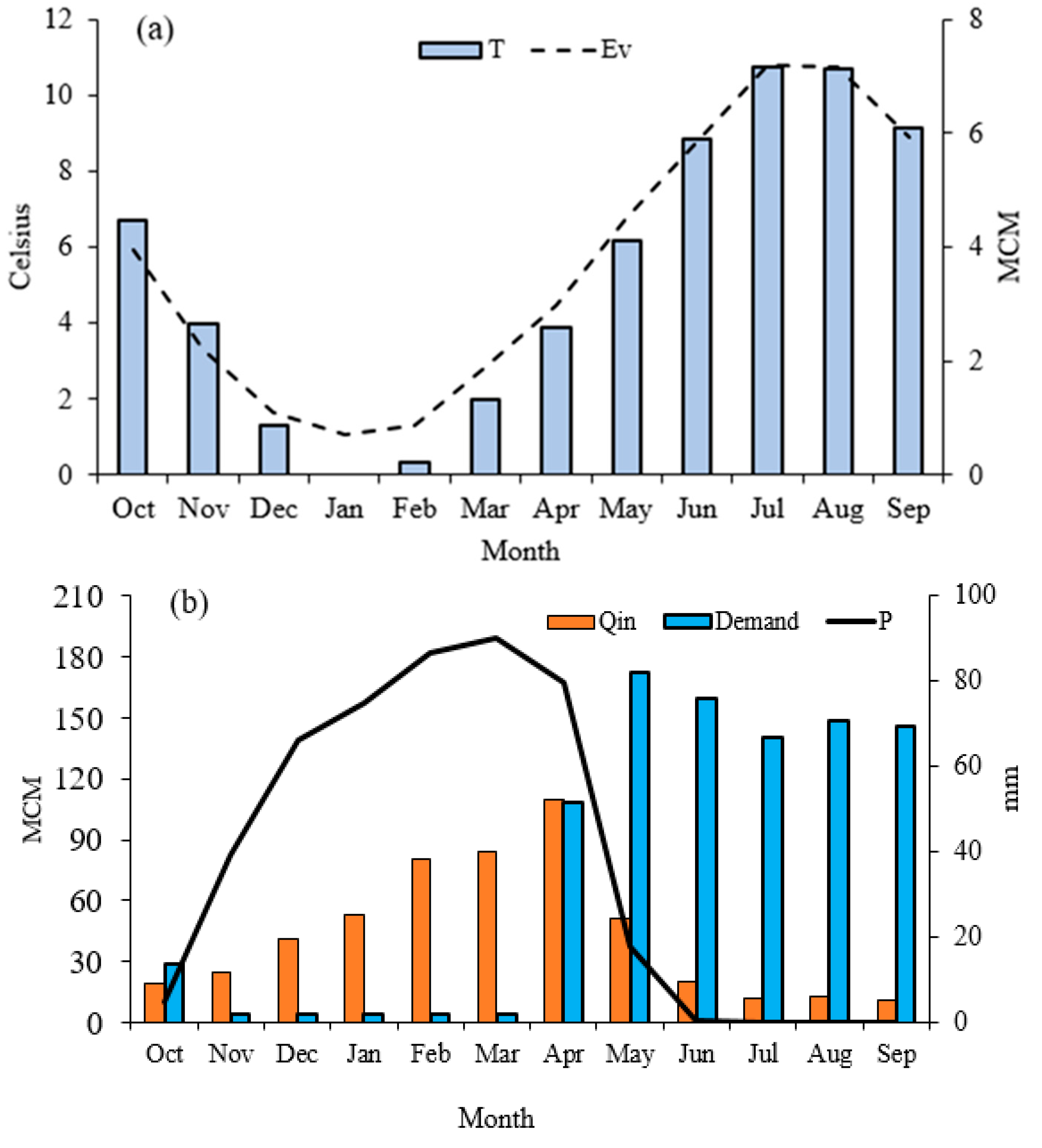
2. Study Area and Data
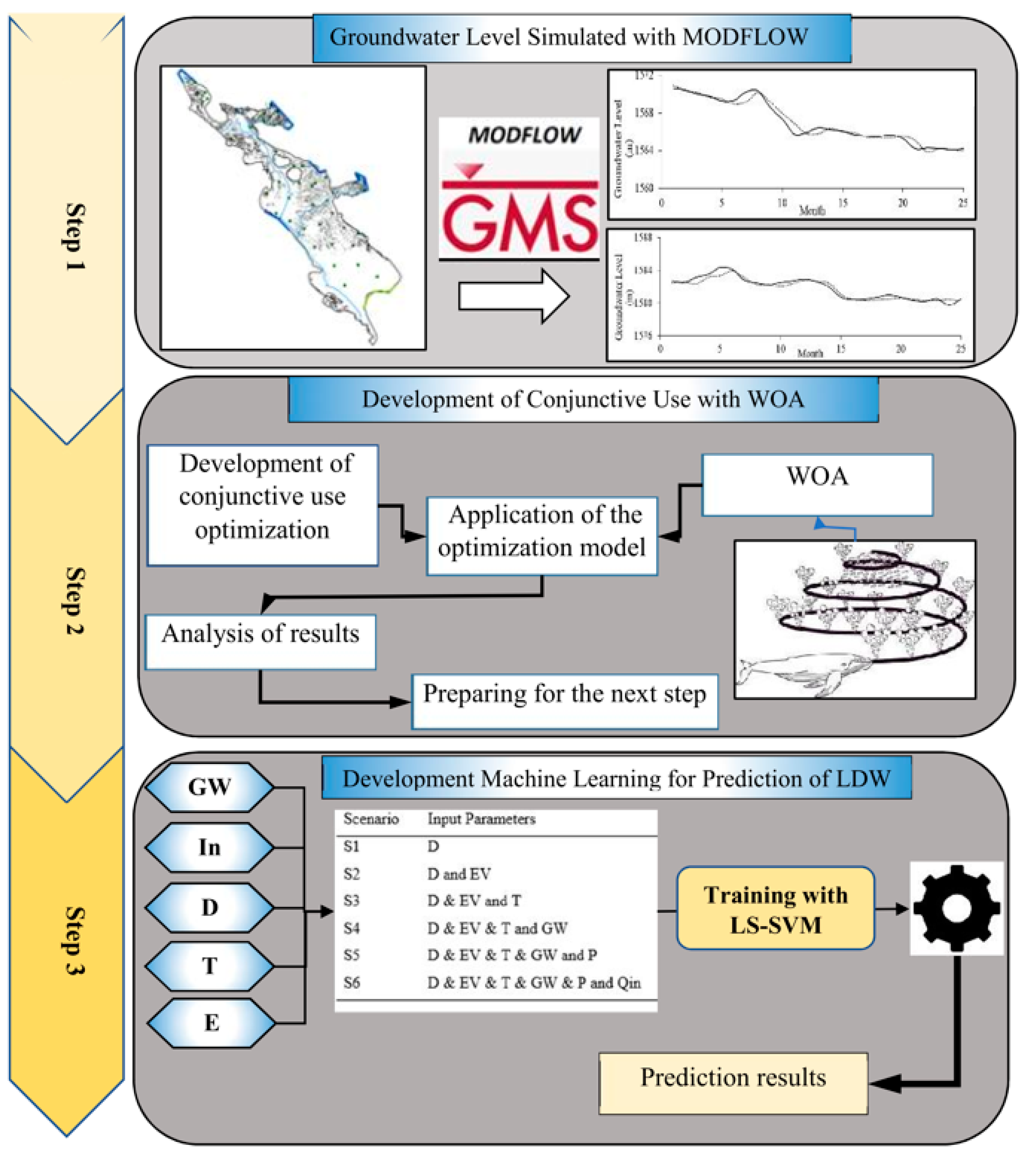
Located in southern Iran, Marvdasht covers an area of about 3941 km2 and lies between 29°19 N to 30°25′ N and 52°15′ E to 53°27′ E (Figure 1). Within this region, the Marvdasht aquifer covers an area of about 1221.5 km2. The main recharge sources of the aquifer are groundwater inflows, precipitation, surface runoff, and return water from agriculture, drinking, and industry wells. The main discharges from the aquifer are through exploitation wells and aqueducts, evaporation, and drainage. The annual recharge of the aquifer is about 480 million cubic meters (MCM). In the last decade, there has been a downward trend in recharge, and during the last 16 year period (2005–2020), the average level of the aquifer has decreased. There has been a drop of about 12 m in the water table, which, in some parts of the aquifer, may drop to about 15 m or more (Figure 2). Adjacent to the groundwater source, the Doroudzan dam is located about 100 km northwest of Shiraz, at the crossing of the Kor River. By regulating about 760 MCM of water annually, the dam supplies about 76,000 ha of the farmlands in the region. A part of the water demand in the aquifer area is thus met through discharge from the dam. Despite the existence of surface water and groundwater resources, these are not used in an optimized conjunctive form.
The overall slope of the aquifer is from the north to the south. The borders of the aquifer entrance fronts are common with the borders of the highlands (Figure 1). Many rivers begin at highlands and pass through the aquifer to other aquifers, from which Sefidrud is of great importance. Therefore, these rivers play a role in charging or discharging the aquifer. The groundwater level is monitored by about 42 observation wells throughout the aquifer. The groundwater simulation was calibrated according to the water level of these wells. There are also a large number of exploitation wells in the aquifer area, which extract an average of about 480 MCM of groundwater annually. Most of this water use is for agricultural purposes (about 80–85%). Due to the existence of surface and groundwater resources, however, the rate of groundwater decline in recent years is evident. Therefore, optimal use of surface and groundwater resources in this area seems necessary.
The time-series data related to air temperature, evaporation, precipitation, demand water, and water inflow to the reservoir during the study period are shown in Figure 3. This information indicates a very similar trend for air temperature and evaporation changes during the study period (Figure 3a). Both variables achieved their highest levels during June, July, August, and September (summer). One can also see that while the amount of evaporation during the nonagricultural months was small (Figure 3b), it reached about 80 MCM in agricultural months. The increase in water demand from March to April indicates that large amounts of surface and groundwater resources are required to supply water demand during the early part of the growing season. Further, during the study period, the inflow to the reservoir gradually increased from October to April, and then tended to decrease due to the sharp decrease in rainfall during the summer months. Therefore, it should always be taken into account in water resources management that when the water demand increases, the amount of rainfall and inflow to the reservoir also decreases significantly. This leaves a significant percentage of water demand unanswered depending on climatic conditions. However, in nonagricultural months, due to increased rainfall, and reduced temperature and evaporation, and with the increase in the amount of inflow to the dam reservoir, water from the reservoir sometimes needs to be released to the surrounding lands. As a result, the allocation of surface water and groundwater resources should follow the principles that always meet the maximum demand.

3. Methodology

The modeling approach proposed here consisted of three main steps (Figure 4). In the first step, the groundwater level was simulated using the modular finite-difference flow (MODFLOW) model to achieve the optimal level of groundwater withdrawal each month of the study period. In the second step, the conjunctive use of water was addressed using the WOA, and the results were evaluated for the study period. In the third step, the LS-SVM model was trained based on various combinations of input variables and the scenarios defined, and was applied to predict the monthly water shortage in the study area. The following subsections describe our methodology in more detail.

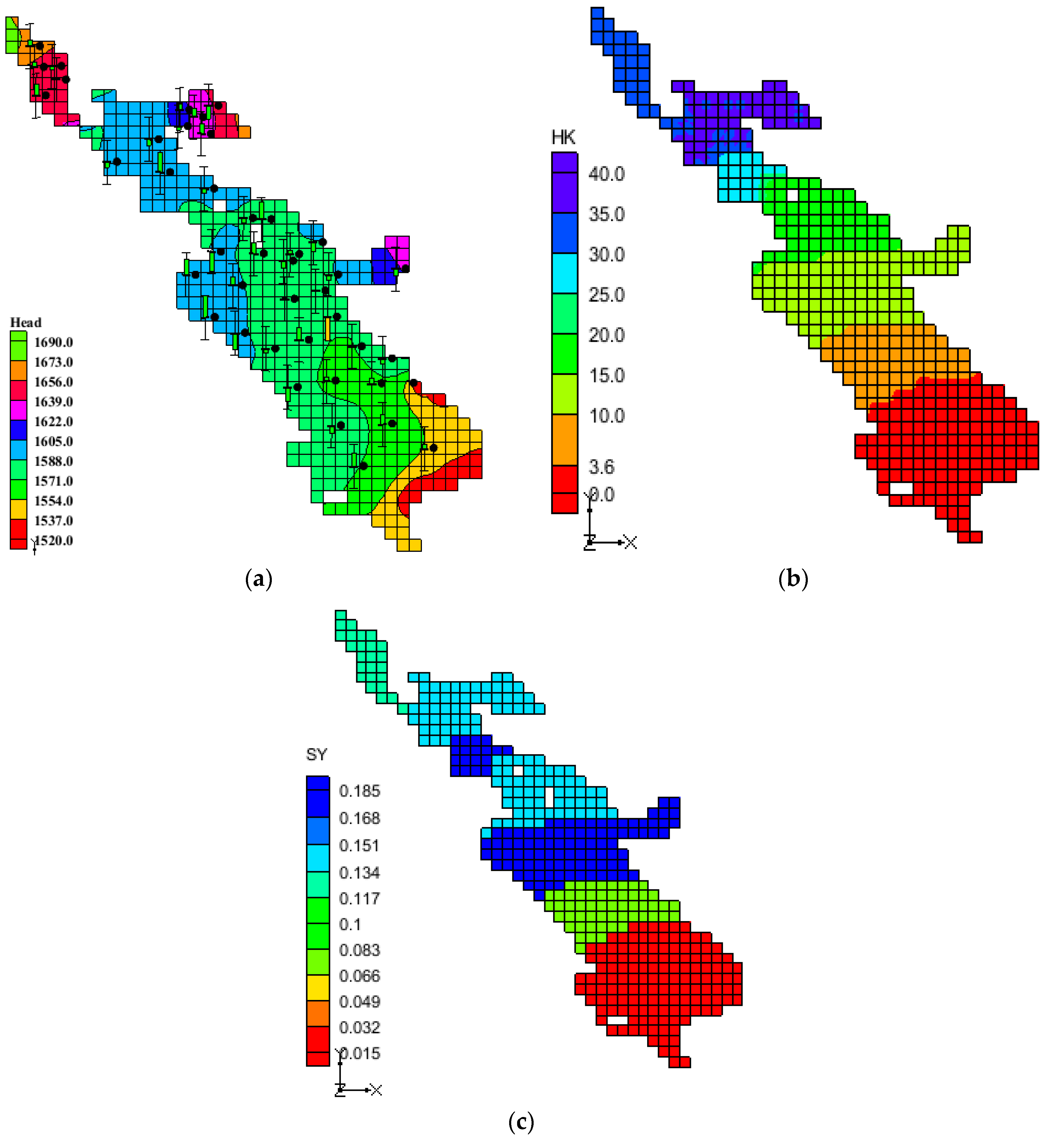
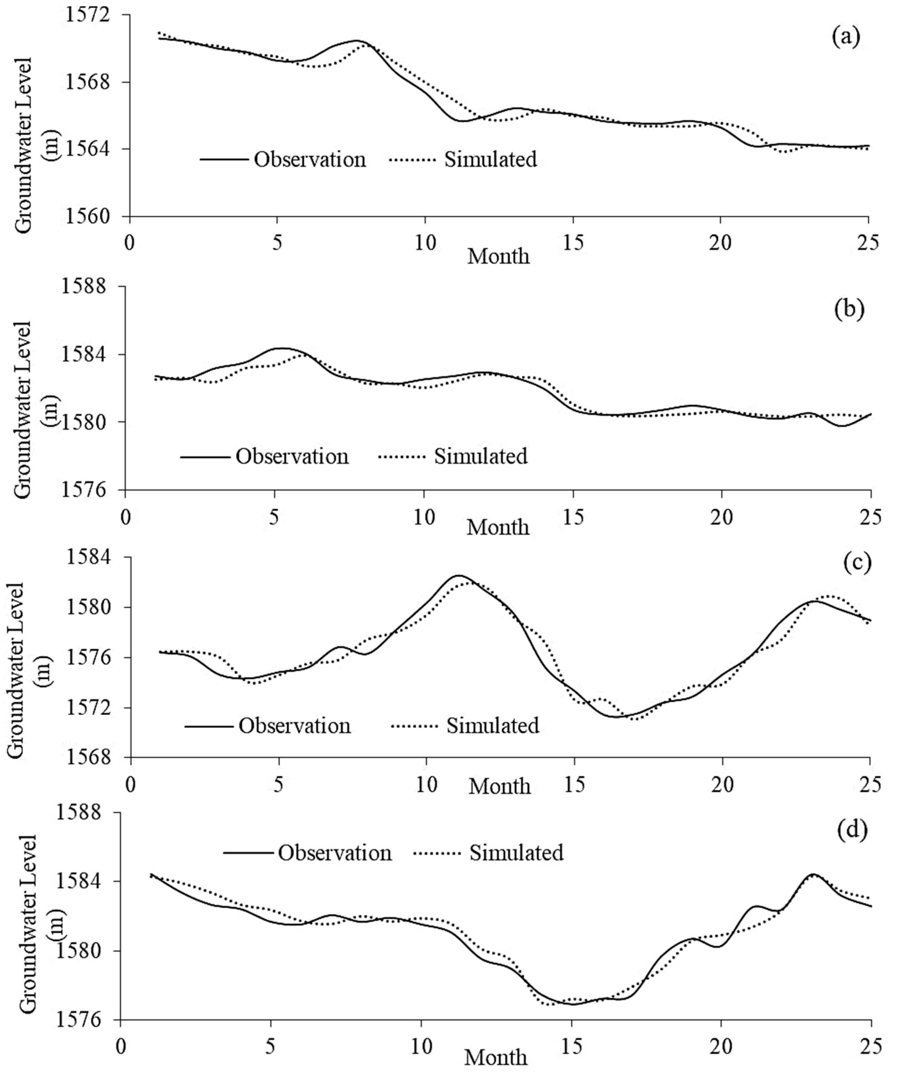
3.1. Groundwater Level Simulation

This model was used to control how much groundwater could be withdrawn and the declining level of groundwater. Aquifer modeling needed information about the water levels from observation wells, the aquifer recharge rate, the river levels, the bedrock and topography (elevation), potential aquifer transmissibility, the hydraulic conductivity, and the initial specific yield. The aquifer is single-layered and free-type. Due to its small width, the thickness of the aquifer is ca. 50 to 80 m on the sides, and ca. 150 to 200 m in the center. There are about 45 observation wells throughout the aquifer that are responsible for controlling the groundwater level.
Hydraulic conductivity was calibrated for the stable status for October 2010, and specific yield values were determined for the unsteady status for two years from October 2010 to September 2012. Afterward, the model was validated using data from 2013–2014. After model building and validation, the model was applied to the five years between 2010 and 2015. The groundwater level of the Marvdasht aquifer was then simulated using the MODFLOW 2000 model within the GMS software [4,51]. This model is one of the most reliable and widely used tools that simulate underground flows based on finite difference methods [51].

3.2. Conjunctive Use Optimization

3.2.1. Objective Function

The main objective was to minimize the yearly water shortage. Accordingly, the objective function and constraints for the study period (the water year 2004–2005 through the water year 2019–2020) were formulated in monthly steps as follows:
M i n   Z = i = 1 16 j = 1 12 ( D e m a n d i j S u p p l y i j ) 2 ( S u p p l y i j = S W i j + G W i j )
Subject to
G W i j Q max i j ,   ( i , j )
G W i j Q min i j ,   ( i , j )
1 j = 12 G W i Q max i
S j + 1 = S j + I n j S W j L o s s j S min S j + 1 S max L o s s j = A j × E v j A j = a S j 3 + b S j 2 + c S j + d
0 S W i j C p
where i is the number of years in the study period; j is the number of months in the year, Demandij is the water demand in year i and month j (MCM); SWij is the surface water exploitation volume (MCM); GWij is the groundwater exploitation volume (MCM); Qmax ij, Qmin ij, and Qmax i are the maximum amount of groundwater withdrawal in year i and month j, the minimum amount of groundwater withdrawal in year i and month j, and the maximum annual withdrawal, respectively. Sj+1, Sj, Smax, and Smin are the reservoir volume at the end of month j, the reservoir volume at the beginning of month j, the maximum storage volume of the reservoir, and the minimum storage volume of the reservoir, respectively. Inj and Lossj are the inflow to the reservoir and losses from the reservoir surface, respectively, during month j. A(j) is the reservoir surface in month j (km2); Evj is the net evaporation difference between precipitation and evaporation in month j; and a, b, c, and d are constant coefficients of the reservoir surface-volume equation. Cp is the maximum water transfer capacity from the dam to the agricultural lands.
The five constraints defined in this study describe (1) the amount of monthly groundwater drop (Equation (2)), (2) the amount of monthly groundwater rise (Equation (3)), (3) the amount of annual groundwater exploitation (Equation (4)), (4) the establishment of a dam continuity relationship to control the amount of surface water allocation and the reservoir volume of the dam in each month and year (Equation (5)), and (5) the maximum water capacity of the canal (Equation (6)). The performance of the developed algorithm was evaluated in three different periods in which the amount of inflow to the dam reservoir varied. In the first period (a), the long-term average values were considered (average period of 15 years). The second period involved the lowest inflow to the dam (2016). Finally, the third period was considered to be the time with the highest inflow to the reservoir (2006).

3.2.2. Whale Optimization Algorithm (WOA)

The WOA is a nature-inspired combinatorial optimization algorithm proposed by Mirjalili and Lewis [52] that operates based on the bubble-net hunting strategy of humpback whales. During hunting, each whale releases air bubbles under the sea to disorient and corral a school of small fish such as salmon, krill, or herring. When the preys go to the center of the bubble circles, the whale hunts and eats a large number of them.
The whale can detect the position of the prey and thus surround the prey. However, as the optimal position of search space is unclear, the whale assumes that the best current answer is the adjacent prey. After determining this point, the search for other optimal points and position updates continues, given by:
D = | C   X t * X t |
X t + 1 = X t * A . D
where t is the current iterator, C and A are the coefficient vectors, X* is the best position vector so far, and X is the position vector. The vectors A and C are calculated as follows:
A = 2 a r a
C = 2 r
where the vector a is a vector in both exploration and exploitation phases and is reduced from 2 to 0 per repetition. The vector r is a random vector in the range between 0 and 1 (Mirjalili and Lewis, 2016). The WOA is a p-metaheuristic combinatorial optimization process, where a population of feasible (usually) solutions is modified through various means to direct the entire set, and a single solution in particular, toward the optimal solution. It seeks, but does not guarantee, optimality.
As illustrated in the research methodology flowchart (Figure 4), we used the WOA to solve the objective function (Equation (2)) given the defined constraints (Equations (3)–(6)) for calculating the amount of allocation of surface and groundwater resources (i.e., conjunctive use) for different periods.

3.3. Prediction of Water Shortage

Several scenarios were developed to predict water shortage by combining the influential input variables. To do so, we first calculated the Pearson’s correlation coefficient of each variable with the target (i.e., water shortage) that revealed that the variables demand (D) and evaporation (Ev) with correlation coefficients of 0.69 and 0.62 had the highest correlation with water shortage. In contrast, precipitation (P) and inflow to the reservoir (Qin) with values of −0.33 and −0.25 were negatively correlated with water shortage (Table 1).
The variable with the highest correlation coefficient with the target was used in the first scenario. The second scenario was developed by combining the first scenario with the variable whose correlation coefficient ranked in second place. Repeating the process produced four other different input scenarios (Table 2). Each scenario was incorporated into the least squares-support vector machine (LS-SVM) model, and the model outputs were evaluated to determine the best input scenario for the prediction of water shortage.

Least Squares-Support Vector Machine (LS-SVM)

Suykens and Vandewalle [53] introduced LS-SVM to decrease the computation complexity and improve the accuracy and performance of classic SVM. Given a set of training data such as { x k ,   y k } K = 1 N , whose input and output data include x k R N and y k R , respectively, Equation (11) shows the nonlinear regression function in the initial weighting [53].
y ( ( x ) ) = W T φ ( ( x ) ) + b
where T, b, and W are the weight, regression bias, and transpose operator, respectively. φ (x) is the nonlinear mapping of inputs in high-dimensional feature space. This nonlinear regression can be solved by minimizing the following objective function.
min j   ( w , e ) = 1 2 W 2 W + 1 2 γ k = 1 N e k 2 min j ( ( w ,   e ) ) = 1 2 W 2 W + 1 2 γ k = 1 N e k 2
Subject to
y k = W T φ ( x ) + b + e k ,         k = 1 ,   , N
where γ is the regulator parameter for the error e. γ always controls the approximation function, so the larger the γ value, the higher the error is.
The equation is solved using the Lagrangian form of the main objective function:
L ( w ,   b ,   e ,   a ) = j ( w , e ) i = 1 N α i { W T φ ( x k ) + b + e k y k } oev
where αi is the Lagrangian coefficient.
Based on the Karush–Kuhn–Tucker condition, the LS-SVM model is written for the approximation function:
y ( x ) = k = 1 N α k K ( x ,   x k ) + b  
where K (x, xk) is the kernel function. In this study, the Gaussian kernel function (Equation (16)) was used.
K ( x ,   x k ) = exp ( | | x x k | | 2 σ 2 )
As mentioned earlier, each one of the six scenarios defined in this study (Table 2) was incorporated into LS-SVM, and the outputs were evaluated to determine the best input scenario for the prediction of water shortage per month for different periods. To do so, 70% of data were randomly selected and used for model training, and the remaining 30% were set aside for model evaluation.
To evaluate the model performance and output, we used the coefficient of determination (R2), root-mean-square error (RMSE), mean absolute percentage error (MAPE), and Nash–Sutcliffe Index (NSE). These metrics are expressed as follows [54,55,56]:
R 2 = 1 i = 1 n ( x p x o ) 2 i = 1 n ( x o x ¯ o ) 2
RMSE = 1 N i = 1 N ( x o x p ) 2
MAPE = 1 N i = 1 N | x o x p x o |
NSE = 1 i = 1 n ( x o x p ) 2 i = 1 n ( x o x ¯ ) 2
where xo is the observed value (i.e., water shortage in the past), xp is the predicted value (i.e., water shortage in the future), x ¯ is the average of the total observation data, and n is the number of samples. The lower RMSE and MAPE and higher NSE and R2 indicate better model performance for the prediction of water shortage in the future.

4. Results and Discussion

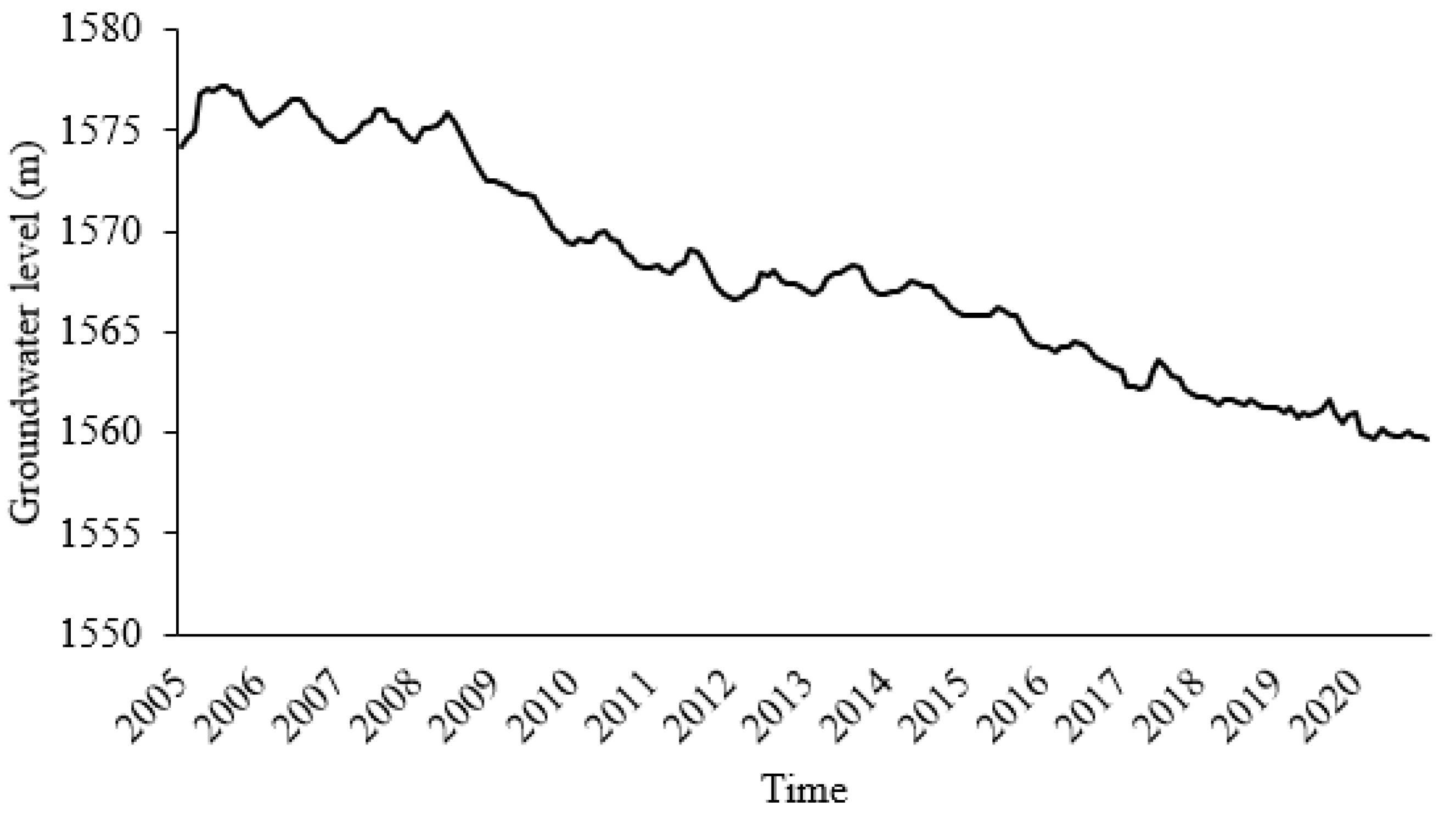
4.1. Simulation Results

Groundwater level was simulated to control the amount of groundwater withdrawal obtained from the optimization model results. The simulation was performed in two steady and unsteady conditions, and the results demonstrated an appropriate simulation performance for both steady and unsteady conditions (Table 3). Further, to ensure the efficiency of the groundwater simulation, we applied the model to the validation data that resulted in an RMSE, MAE, and R2 of 1.1 m, 0.93 m, and 0.98, respectively.
The condition of the observation wells showed that there was an acceptable correlation between the observed and simulated values in each observation well, which indicates the low simulation error (Figure 5a). Further, the groundwater level varied from 1520 to 1690 m.
Figure 5b shows the calibrated values of hydraulic conductivity and storage coefficient in both steady and unsteady states. The maximum value of hydraulic conductivity was about 35 m/day in the northern regions of the aquifer. Due to the sedimentation of fine particles, the lowest hydraulic conductivity values were observed in the south of the aquifer. The specific yield always varied between 2 and 19%, while this value was in the range of 6 to 12% in the central portion of the aquifer (Figure 5c). Finally, various withdrawals were performed on the simulation model. The maximum groundwater withdrawal values in each month were determined after calculating the groundwater level drops and considered as the constraints of the optimized conjunctive model.
The trend of changes in the simulated and observed groundwater level demonstrates that the MODFLOW code was able to successfully simulate groundwater level (Figure 6). Due to a large number of observation wells, point_30, 40, 23, and 25 were randomly shown as the samples in order to show observed and simulated values in such wells. Given the difference in numbers on the y-axis, it is obvious that there was a much smaller difference between the two values. Moreover, the time series of both values indicate that the trend was correctly detected by the MODFLOW code.

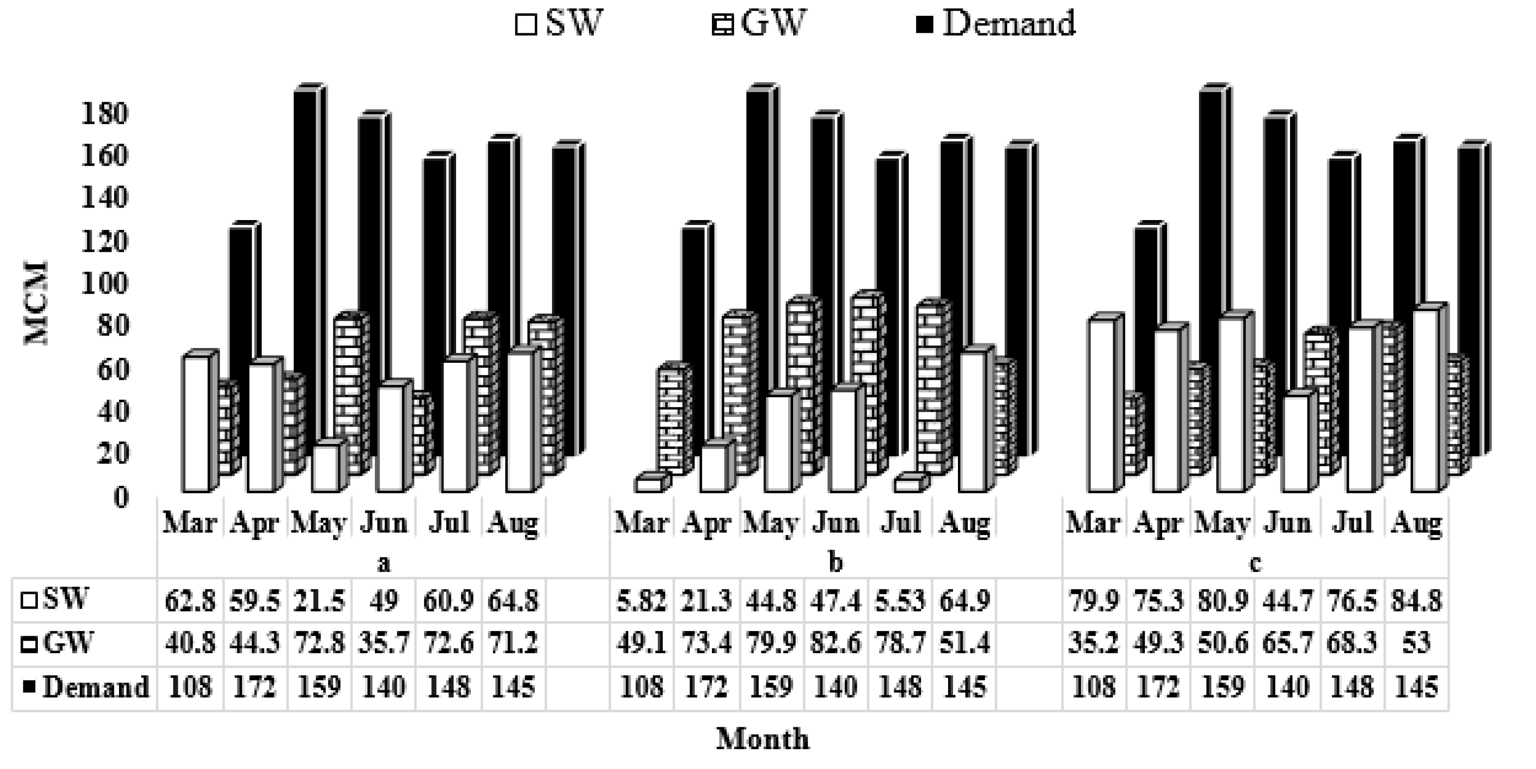
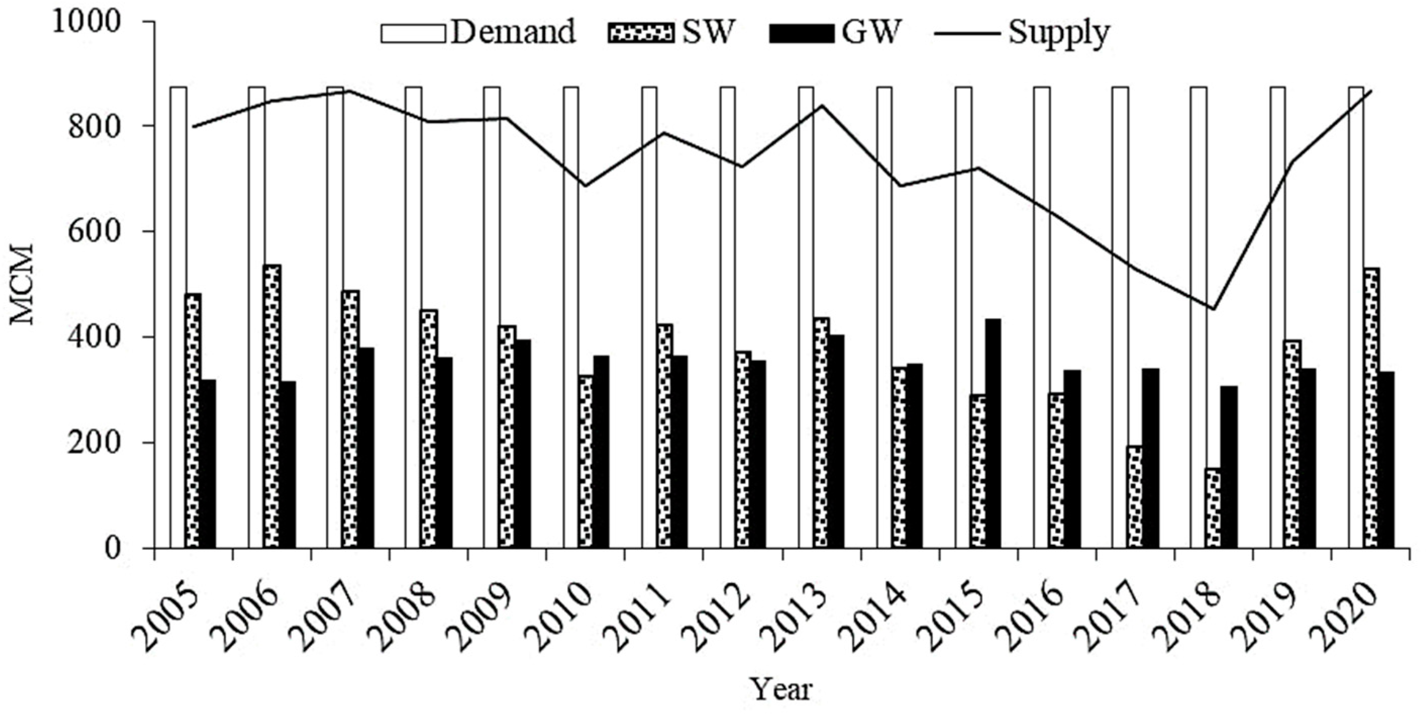
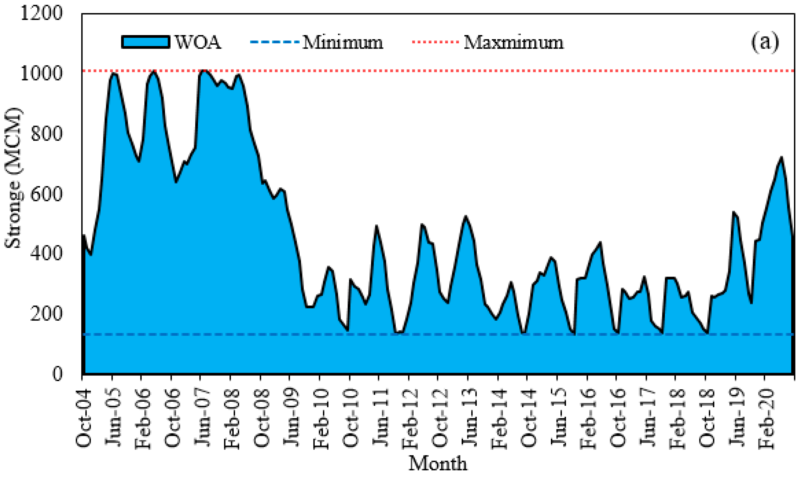
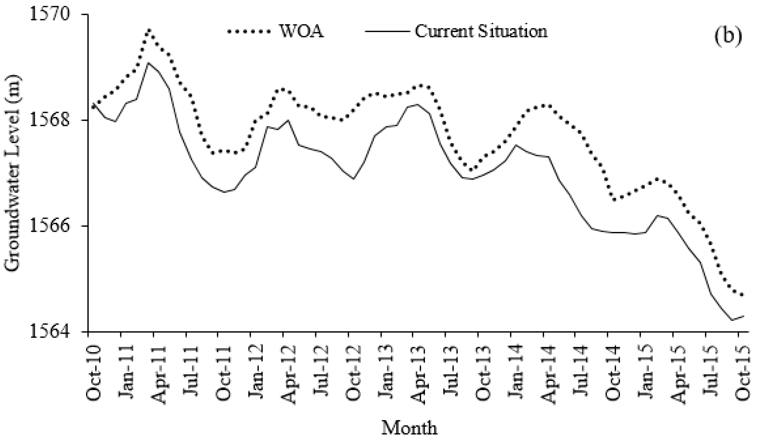
4.2. Optimization Results

The best parameter values of the WOA were obtained after running the algorithm several times. The a and r parameters were adjusted at 0 to 2 and a random vector in [0, 1], respectively. Among different population sizes (25, 30, and 50) considered for the implementation of the algorithm, the population size of 30 performed best. The WOA algorithm was performed in 2500 iterations because no improvement was achieved after iteration 2500. Depending on the type of period considered, the performance of the optimization model was different in allocating the amount of surface water and groundwater. In period b, water demand was mainly met from groundwater sources (Figure 7). Further, during this period, as the inflow amount was much lower than the long-term average, to meet the maximum water demand, groundwater withdrawal values were considered to be 10 to 15% higher than regular and wet periods, respectively. However, in period c, most of the water demand was met through the dam. The difference between the allocation values of groundwater in the two periods b and c was relatively large (Figure 7). In fact, when the system was considered for a dry period, the optimization model used the maximum groundwater resources to meet the water demand.
In contrast, in the wet periods and when the amount of inflow to the dam reservoir is sufficient, the model used more surface water resources, and to some extent, it allowed the aquifer to move forward to compensate for the reservoir shortages, and this is one of the valuable points of the approach of conjunctive use of surface and groundwater resources. In period A, the allocated amounts of both surface water and groundwater sources were slightly different from the other two periods. In this case, depending on the average amount of inflow to the reservoir, in some months, the amount of allocated surface water was higher than that of groundwater and is less in other months. For example, in April, when water demand is highest each year, the allocated amounts in the period a were 63 and 41 MCM for surface water and groundwater, respectively. In comparison, these values for the allocated amount of surface water and groundwater were 6 and 49 MCM, respectively, in period b, but in period c, the allocation to surface water was 79 MCM and to groundwater was 35 MCM. By examining the allocated amounts in the three periods, it can be stated that the model, in addition to meeting the maximum water demand, created a balance between groundwater and surface water so that both the groundwater reservoir shortage is partially compensated and the exploitation from surface water sources is maximized. In general, in wet years, the optimization model emphasized more on surface water, and in times of drought or when the amount of inflow to the dam reservoir is minimal, it used more groundwater resources. Figure 7 shows these results for the agricultural months.
After evaluating the optimization model for three different periods, the application of the model was extended to a 16 year period with monthly steps (Figure 8). As can be seen in Figure 8 and Table 4, 50% of water demand was met by surface water in 20 years. Between 2013 and 2018, when the inflow amount to the dam was lower, 51 to 67% of the water demand was met by groundwater (Table 4). The highest use of groundwater resources occurred in 2018, in which about 67% of water demand was met by groundwater resources. From the early years of the study period to 2014, the percentage of groundwater exploitation to meet the water demand was less than 50%, the exact amount of which varied between 37 and 49%. According to the optimization results, the logic of conjunctive use of surface water and groundwater resources was observed by the developed model. However, according to Table 4, the highest water demand was met in 2007 and 2020, when about 99% of demand was met with the share of surface and groundwater resources being 56 and 44% in 2007, and 61 and 39% in 2020, respectively. Further, the highest water shortage during the study period occurred in 2018, in which about 52% of water demand was met, with the share of groundwater (67%) and surface water (33%).
When allocating surface water resources from dams and groundwater resources, the remaining volume of reservoirs should always be considered. In other words, the allocations should be such that surface and groundwater resources are not damaged. Therefore, the volume of resources was calculated after allocating the amounts in each month. One of the constraints of the optimization model was that the allocation of the reservoir should not be more than the capacity of the water supply channel, and the other was the continuity equation. Figure 6 shows the changes in the reservoir volume after allocating the amount of surface water in each month. The reservoir volume has always varied between its maximum (1030 MCM) and minimum (133 MCM) capacity (Figure 9a).
In the early years, when the amount of inflow to the dam reservoir was high, the reservoir volume was in good condition. However, since 2010, the reservoir volume has decreased over time, reaching its lowest level in 2016–2018. During these years, we observed the most significant shortage of water supply. Nonetheless, from the end of 2019 to 2020, the reservoir volume exerted an upward trend. On the other hand, changes in groundwater level are slightly different from the reservoir volume. During the study period, the aquifer’s level decreased by about 12 m, which is an average of about 75 to 85 cm per year. By applying the optimal use from the beginning of the period to the end of groundwater simulation, we saw groundwater rising by about 0.66 m (Figure 9b).
Applying the results of the optimization model on the groundwater level simulation during the simulated period (about 5 years) revealed that the groundwater level increased in the first months of the simulation period, and it was also clear that the suggested optimization model was able to affect the groundwater drop changes. A slight increase in the groundwater level was obvious in the years in which groundwater resources were overused caused by extra allocation (such as 2015–2016). Despite the extra allocation of groundwater resources in the final years of groundwater simulation, the groundwater level rose compared to the status quo. This indicates that in the optimal integrated groundwater model, groundwater uses its stored volume captured in nondrought wet months of the year in months when surface water resources are available in small quantities. In special circumstances, not only does it satisfy the maximum water demands, but serious damage is also not done to groundwater.
It should be kept in mind that to achieve proper stability, we need more extended periods to continue the current optimization process for complete compensation of groundwater level loss in the aquifer. However, the model somehow prevented the downward trend of groundwater level to some extent, which also caused a relative rise in groundwater level. This is a promising result for water scientists and experts who are concerned about the environment. In general, the results showed that by relying on both water supply sources and maintaining the reservoir volume to a certain extent, the amount of groundwater level drop could also be controlled by the model. This requires the participation of farmers, managers, and communities.

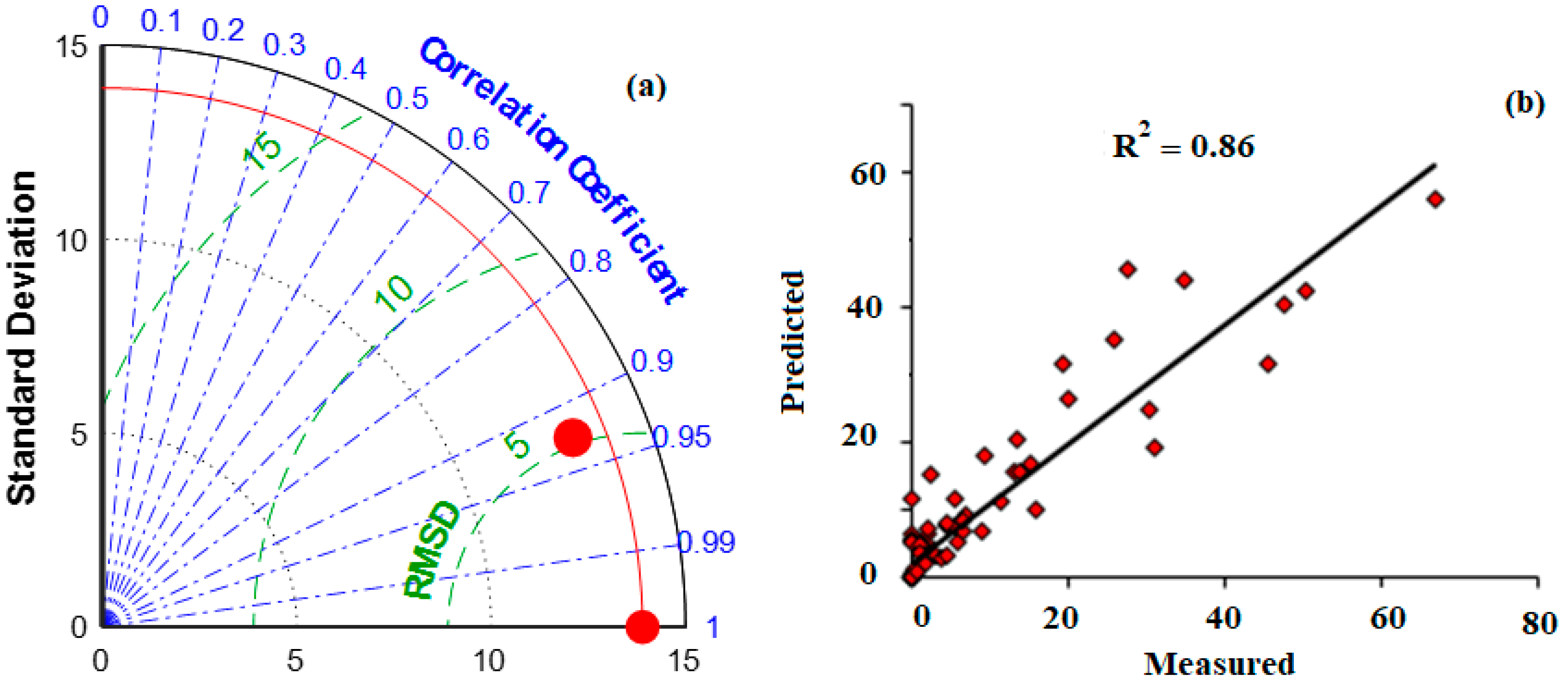
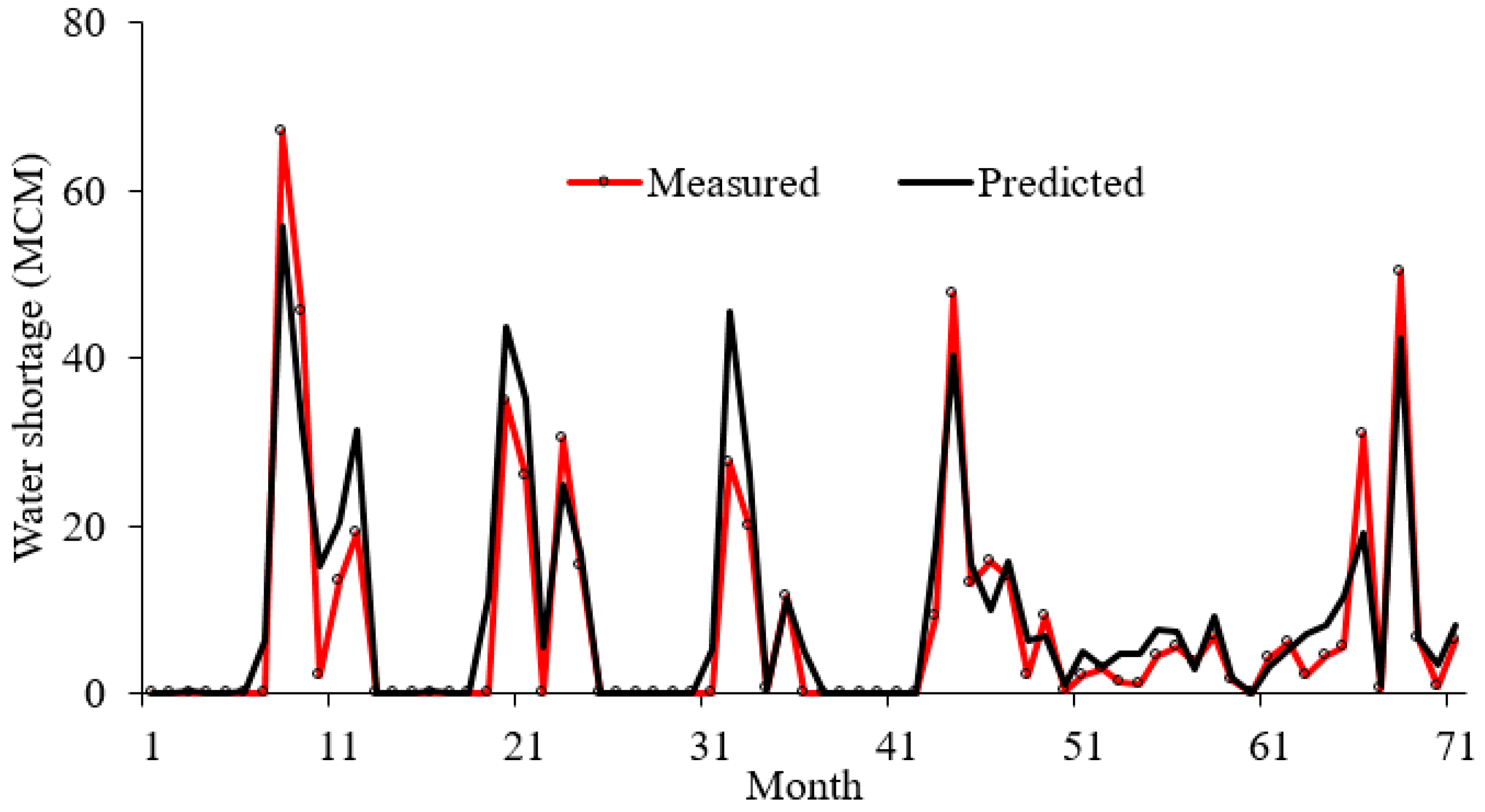
4.3. Prediction Results

In the prediction phase of the methodology, the amount of water shortage was predicted based on the optimization results. The optimization model was applied to 12 months of the 16 year period, and the amount of water shortage in each month was estimated. These values were then predicted using the input scenarios consisting of different combinations of groundwater withdrawal, precipitation, temperature, and water demand in each month. Each of the input scenarios was implemented by LS-SVR, the results of which can be seen in Table 5. Among the developed scenarios, the sixth scenario, which included all input variables, was selected as the most appropriate model to predict the amount of monthly water shortage with an RMSE, MAPE, and NSE of 5.70 MCM, 3.43 MCM, and 0.89, respectively, for the test data. The lowest testing performance was observed for the first scenario, which included only one variable (water demand). In this scenario, RMSE, MAPE, and NSE were 21.93 MCM, 13.65 MCM, and 0.58, respectively, indicating a poor performance because of using one input variable to predict water shortage. In addition to the sixth scenario, having the values of the variables of the fourth scenario, it was possible to achieve relatively acceptable testing performance for predicting water shortage with an RMSE, MAPE, and NSE of 6.30 MCM, 4.60 MCM, and 0.88, respectively.
Taylor’s diagram was also used to examine the predictions (Figure 10a). This diagram shows the standard deviation of predictions on the horizontal and vertical axes and the correlation coefficient on the arc. Further, the arcs drawn inside the quadrant indicate the root-mean-square deviation (RMSD). The lower the RMSD and the higher the correlation coefficient of a model in Taylor’s diagram, the more accurate the predictive performance. The results of Taylor’s diagram show that the correlation coefficient and RMSD between the measured values and the LS-SVM predictions were greater than 0.93 and lower than 95, respectively. The standard deviation of the LS-SVM model was ca. 13, which was much closer to the standard deviation of the measured data. The scatterplots of the measured and predicted values are shown in Figure 9b. LS-SVM resulted in the highest performance (R2 = 0.86). Moreover, the data were close to the bisector line in the LS-SVM model, which reveals its small prediction error.
Investigating the time series of measured and predicted data for the testing dataset obtained from the selected scenario by model made the analysis and behavior of the predicted values more accurate. Figure 11 shows that LS-SVM correctly detected the changes in water shortage in almost all study months, although a few over-predictions were evident in some months (e.g., months 11, 21, and 31). Overall, the results demonstrated the capability of LS-SVM for predicting the minimum and maximum changes in the water shortage.
With this approach, it was possible to forecast a monthly water deficit with acceptable accuracy. This prediction will allow farmers to avoid losses and help decision-makers choose a wise water allocation. The study results and model assessment validated the prediction approach. Additionally, this study, along with [36], used a Bayesian model to codify instructions for autonomous allocation rules, and [6,41] applied ANFIS, FIS, and hybrid ANFIS models adequately to abstract groundwater. In their research, machine learning models were presented as an appropriate tool to predict some parameters with the help of optimization model results. Based on this investigation and the previous studies discussed above, an intelligent, holistic model utilizing optimal conjunctive results can be constructed, which can help allocate water resources efficiently and predict water deficits monthly. Even though the amount of groundwater abstraction prediction depends on various factors such as the amount of groundwater that declined in the previous month and the current month, its estimation is a problematic issue. Thus, this study attempted to predict groundwater deficits that were not caused by groundwater abstraction, which was not considered in the modeling. However, the prediction of each case is tied to the availability of data, conditions, and site.

5. Conclusions

In this study, a three-step methodology was proposed for the optimization of conjunctive use of surface water and groundwater resources. This approach was implemented in the Marvdasht region, Iran, which includes both surface water and groundwater systems. The optimized conjunctive model was investigated in three different periods to determine its performance. The selection of the LS-SVM model over the optimization model for the prediction of water shortage decreased the computation complexity that enables water managers to achieve the necessary information without spending much time. This approach is applicable to other areas with surface water (river or dam) and groundwater (aquifer).
This study showed that using a simulation-optimization approach that imposed some constraints for groundwater exploitation improved the groundwater status in the area so that during the simulation period, the groundwater level increased by about 0.7 m. The results of LS-SVM showed that machine learning models are a reliable tool for predicting the volume of water needs or the amount of groundwater use. In addition, with the help of variables such as groundwater exploitation, precipitation, temperature, and water demand in each month, it is possible to predict the amount of monthly water shortage in similar areas. This approach is applicable in other study areas. Therefore, relying on scientific approaches and using existing tools for simulation, optimization, and forecasting, the performance of a system can be evaluated in real and actual problems, and an appropriate management decision can be made in the shortest possible time, which is valuable for decision-makers and managers. The lack of zoning of the aquifer and review of optimization results in different areas of the aquifer was one of the limitations of this study, which was not feasible, due to the narrow width of the aquifer. Thus, in future research, for aquifers that are wider, an optimal amount of surface and groundwater resources can be allocated in each area of the aquifer.
Simultaneous use of the heuristic model’s results and field data to predict water shortage distinguishes this study from previous works reported in the literature. This prediction enables managers and researchers to make more informed decisions in response to future water shortages. Based on the results of this study, we recommend using this simulation-optimization approach for conjunctive water planning in other regions. We also recommend extending the analysis to use the status of groundwater quality, the effect of climate change on water needs, and evaluating other machine learning methods and optimization algorithms for testing the possibility of improving the quality of results.

Author Contributions

Conceptualization: Z.K., S.G.M. and N.A.A.; data collection: Z.K., S.G.M. and N.A.A.; formal analysis: Z.K., S.G.M. and N.A.A.; validation: Z.K., S.G.M. and N.A.A.; supervision: S.G.M. and A.J.; writing—original draft: all authors; APC: P.B. and A.J. All authors have read and agreed to the published version of the manuscript.

Funding

This research received no external funding.

Institutional Review Board Statement

Not applicable.

Informed Consent Statement

Not applicable.

Data Availability Statement

The data presented in this study will be available on interested request from the first corresponding author.

Conflicts of Interest

The authors declare no conflict of interest.

References

  1. Ekwueme, B.N.; Agunwamba, J.C. Modeling the influence of meteorological variables on runoff in a tropical watershed. Civ. Eng. J. 2020, 6, 2344–2351. [Google Scholar] [CrossRef]
  2. Ekwueme, B.N.; Agunwamba, J.C. Trend Analysis and variability of air temperature and rainfall in regional river basins. Civ. Eng. J. 2021, 7, 816–826. [Google Scholar] [CrossRef]
  3. Li, X.; Zhang, K.; Gu, P.; Feng, H.; Yin, Y.; Chen, W.; Cheng, B. Changes in precipitation extremes in the Yangtze River Basin during 1960–2019 and the association with global warming, ENSO, and local effects. Sci. Total Environ. 2021, 760, 144244. [Google Scholar] [CrossRef] [PubMed]
  4. Javadi, S.; Saatsaz, M.; Shahdany, S.M.H.; Neshat, A.; Milan, S.G.; Akbari, S. A new hybrid framework of site selection for groundwater recharge. Geosci. Front. 2021, 12, 101144. [Google Scholar] [CrossRef]
  5. Moghaddam, H.K.; Milan, S.G.; Kayhomayoon, Z.; Kivi, Z.R.; Azar, N.A. The prediction of aquifer groundwater level based on spatial clustering approach using machine learning. Environ. Monit. Assess. 2021, 193, 173. [Google Scholar] [CrossRef]
  6. Milan, S.G.; Roozbahani, A.; Azar, N.A.; Javadi, S. Development of adaptive neuro fuzzy inference system –Evolutionary algorithms hybrid models (ANFIS-EA) for prediction of optimal groundwater exploitation. J. Hydrol. 2021, 598, 126258. [Google Scholar] [CrossRef]
  7. Pan, D.; Chen, H. Border pollution reduction in China: The role of livestock environmental regulations. China Econ. Rev. 2021, 69, 101681. [Google Scholar] [CrossRef]
  8. Das, B.; Singh, A.; Panda, S.N.; Yasuda, H. Optimal land and water resources allocation policies for sustainable irrigated agriculture. Land Use Policy 2015, 42, 527–537. [Google Scholar] [CrossRef]
  9. Kadam, A.; Umrikar, B.; Bhagat, V.; Wagh, V.; Sankua, R.N. Land suitability analysis for afforestation in semi-arid watershed of Western Ghat, India: A groundwater recharge perspective. Geol. Ecol. Landscapes 2021, 5, 136–148. [Google Scholar] [CrossRef]
  10. Theis, C.V. The effect of a well on the flow of a nearby stream. Trans. Am. Geophys. Union 1941, 22, 734–738. [Google Scholar] [CrossRef] [Green Version]
  11. Belaineh, G.; Peralta, R.C.; Hughes, T.C. Simulation/optimization modeling for water resources management. J. Water Resour. Plan. Manag. 1999, 125, 154–161. [Google Scholar] [CrossRef]
  12. Karamouz, M.; Tabari, M.M.R.; Kerachian, R. Application of genetic algorithms and artificial neural networks in conjunctive use of surface and groundwater resources. Water Int. 2007, 32, 163–176. [Google Scholar] [CrossRef]
  13. Safavi, H.R.; Esmikhani, M. Conjunctive use of surface water and groundwater: Application of Support Vector Machines (SVMs) and genetic algorithms. Water Resour. Manag. 2013, 27, 2623–2644. [Google Scholar] [CrossRef]
  14. Yousefi, M.; Banihabib, M.E.; Soltani, J.; Roozbahani, A. Multi-objective particle swarm optimization model for conjunctive use of treated wastewater and groundwater. Agric. Water Manag. 2018, 208, 224–231. [Google Scholar] [CrossRef]
  15. Soleimani, S.; Bozorg-Haddad, O.; Boroomandnia, A.; Loáiciga, H.A. A review of conjunctive GW-SW management by simulation–optimization tools. J. Water Supply Res. Technol. 2021, 70, 239–256. [Google Scholar] [CrossRef]
  16. Vedula, S.; Mujumdar, P.; Sekhar, G.C. Conjunctive use modeling for multicrop irrigation. Agric. Water Manag. 2005, 73, 193–221. [Google Scholar] [CrossRef] [Green Version]
  17. Chen, Y.W.; Chang, L.C.; Huang, C.W.; Chu, H.J. Applying genetic algorithm and neural network to the conjunctive use of surface and subsurface water. Water Resour. Manag. 2013, 27, 4731–4757. [Google Scholar] [CrossRef]
  18. Landa, S.A. Optimizing Sustainable Integrated Use of Groundwater, Surface Water and Reclaimed Water for the Competing Demands of Agricultural Net Return and Urban Population; Utah State University: Logan, UT, USA, 2016. [Google Scholar]
  19. El-Rawy, M.; Zlotnik, V.A.; Al-Raggad, M.; Al-Maktoumi, A.; Kacimov, A.; Abdalla, O. Conjunctive use of groundwater and surface water resources with aquifer recharge by treated wastewater: Evaluation of management scenarios in the Zarqa River Basin, Jordan. Environ. Earth Sci. 2016, 75, 1146. [Google Scholar] [CrossRef]
  20. Miao, R.; Liu, Y.; Wu, L.; Wang, D.; Liu, Y.; Miao, Y.; Yang, Z.; Guo, M.; Ma, J. Effects of long-term grazing exclusion on plant and soil properties vary with position in dune systems in the Horqin Sandy Land. Catena 2021, 209, 105860. [Google Scholar] [CrossRef]
  21. Thammanu, S.; Marod, D.; Han, H.; Bhusal, N.; Asanok, L.; Ketdee, P.; Gaewsingha, N.; Lee, S.; Chung, J. The influence of environmental factors on species composition and distribution in a community forest in Northern Thailand. J. For. Res. 2021, 32, 649–662. [Google Scholar] [CrossRef]
  22. Peralta, R.C. Simulation/optimization applications and software for optimal ground-water and conjunctive water management. Ground Water Modeling Cent. 2001, 691–694. [Google Scholar]
  23. Barlow, P.M.; Ahlfeld, D.P.; Dickerman, D.C. Conjunctive-management models for sustained yield of stream-aquifer systems. J. Water Resour. Plan. Manag. 2003, 129, 35–48. [Google Scholar] [CrossRef]
  24. Safavi, H.R.; Enteshari, S. Conjunctive use of surface and ground water resources using the ant system optimization. Agric. Water Manag. 2016, 173, 23–34. [Google Scholar] [CrossRef]
  25. Karamouz, M.; Zahraie, B.; Kerachian, R.; Eslami, A. Crop pattern and conjunctive use management: A case study. Irrig. Drain. 2008, 59, 161–173. [Google Scholar] [CrossRef]
  26. Joodavi, A.; Izady, A.; Maroof, M.T.K.; Majidi, M.; Rossetto, R. Deriving optimal operational policies for off-stream man-made reservoir considering conjunctive use of surface- and groundwater at the Bar dam reservoir (Iran). J. Hydrol. Reg. Stud. 2020, 31, 100725. [Google Scholar] [CrossRef]
  27. Zeinali, M.; Azari, A.; Heidari, M.M. Multiobjective optimization for water resource management in low-flow areas based on a coupled surface water–groundwater model. J. Water Resour. Plan. Manag. 2020, 146, 04020020. [Google Scholar] [CrossRef]
  28. Rezaei, F.; Safavi, H.R.; Mirchi, A.; Madani, K. f-MOPSO: An alternative multi-objective PSO algorithm for conjunctive water use management. J. Hydro-Environ. Res. 2017, 14, 1–18. [Google Scholar] [CrossRef]
  29. Sepahvand, R.; Safavi, H.R.; Rezaei, F. Multi-objective planning for conjunctive use of surface and ground water resources using genetic programming. Water Resour. Manag. 2019, 33, 2123–2137. [Google Scholar] [CrossRef]
  30. Rezaei, F.; Safavi, H.R. Sustainable conjunctive water use modeling using dual fitness particle swarm optimization algorithm. Water Resour. Manag. 2022. [Google Scholar] [CrossRef]
  31. Rezaei, F.; Safavi, H.R. f-MOPSO/Div: An improved extreme-point-based multi-objective PSO algorithm applied to a socio-economic-environmental conjunctive water use problem. Environ. Monit. Assess. 2020, 192, 767. [Google Scholar] [CrossRef]
  32. Mehrabi, A.; Heidarpour, M.; Safavi, H.R.; Rezaei, F. Assessment of the optimized scenarios for economic-environmental conjunctive water use utilizing gravitational search algorithm. Agric. Water Manag. 2021, 246, 106688. [Google Scholar] [CrossRef]
  33. Ashu, A.B.; Lee, S.-I. Simulation-optimization model for conjunctive management of surface water and groundwater for agricultural use. Water 2021, 13, 3444. [Google Scholar] [CrossRef]
  34. Safavi, H.R.; Alijanian, M.A. Optimal crop planning and conjunctive use of surface water and groundwater resources using fuzzy dynamic programming. J. Irrig. Drain. Eng. 2011, 137, 383–397. [Google Scholar] [CrossRef]
  35. Liu, L.; Cui, Y.; Luo, Y. Integrated modeling of conjunctive water use in a canal-well irrigation district in the Lower Yellow River Basin, China. J. Irrig. Drain. Eng. 2013, 139, 775–784. [Google Scholar] [CrossRef]
  36. Rafipour-Langeroudi, M.; Kerachian, R.; Bazargan-Lari, M.R. Developing operating rules for conjunctive use of surface and groundwater considering the water quality issues. KSCE J. Civ. Eng. 2014, 18, 454–461. [Google Scholar] [CrossRef]
  37. Singh, A. Simulation–optimization modeling for conjunctive water use management. Agric. Water Manag. 2014, 141, 23–29. [Google Scholar] [CrossRef]
  38. An-Vo, D.-A.; Mushtaq, S.; Nguyen-Ky, T.; Bundschuh, J.; Tran-Cong, T.; Maraseni, T.N.; Reardon-Smith, K. Nonlinear Optimisation using production functions to estimate economic benefit of conjunctive water use for multicrop production. Water Resour. Manag. 2015, 29, 2153–2170. [Google Scholar] [CrossRef]
  39. Yu, L.; Kinzelbach, W.; Li, W.; Pedrazzini, G.; Xin, L. Multi-objective optimization for conjunctive water use using coupled hydrogeological and agronomic models: A case study in Heihe mid-reach (China). In Proceedings of the AGU Fall Meeting, New Orleans, LA, USA, 11–15 December 2017. [Google Scholar]
  40. Aljanabi, A.A.; Mays, L.W.; Fox, P. Optimization model for agricultural reclaimed water allocation using mixed-integer nonlinear programming. Water 2018, 10, 1291. [Google Scholar] [CrossRef] [Green Version]
  41. Milan, S.G.; Roozbahani, A.; Banihabib, M.E. Fuzzy optimization model and fuzzy inference system for conjunctive use of surface and groundwater resources. J. Hydrol. 2018, 566, 421–434. [Google Scholar] [CrossRef]
  42. Xu, J.; Zhou, L.; Li, Y.; Ding, J.; Wang, S.; Cheng, W.-C. Experimental study on uniaxial compression behavior of fissured loess before and after vibration. Int. J. Géoméch. 2022, 22, 04021277. [Google Scholar] [CrossRef]
  43. Xu, J.; Zhou, L.; Hu, K.; Li, Y.; Zhou, X.; Wang, S. Influence of wet-dry cycles on uniaxial compression behavior of fissured loess disturbed by vibratory loads. KSCE J. Civ. Eng. 2022. [Google Scholar] [CrossRef]
  44. He, S.; Guo, F.; Zou, Q.; Ding, H. MRMD2.0: A Python tool for machine learning with feature ranking and reduction. Curr. Bioinform. 2021, 15, 1213–1221. [Google Scholar] [CrossRef]
  45. Kayhomayoon, Z.; Azar, N.A.; Milan, S.G.; Moghaddam, H.K.; Berndtsson, R. Novel approach for predicting groundwater storage loss using machine learning. J. Environ. Manag. 2021, 296, 113237. [Google Scholar] [CrossRef] [PubMed]
  46. Zhao, T.; Shi, J.; Entekhabi, D.; Jackson, T.J.; Hu, L.; Peng, Z.; Yao, P.; Li, S.; Kang, C.S. Retrievals of soil moisture and vegetation optical depth using a multi-channel collaborative algorithm. Remote Sens. Environ. 2021, 257, 112321. [Google Scholar] [CrossRef]
  47. Jaafari, A.; Panahi, M.; Mafi-Gholami, D.; Rahmati, O.; Shahabi, H.; Shirzadi, A.; Lee, S.; Bui, D.T.; Pradhan, B. Swarm intelligence optimization of the group method of data handling using the cuckoo search and whale optimization algorithms to model and predict landslides. Appl. Soft Comput. 2021, 116, 108254. [Google Scholar] [CrossRef]
  48. Zhao, T.; Shi, J.; Lv, L.; Xu, H.; Chen, D.; Cui, Q.; Jackson, T.J.; Yan, G.; Jia, L.; Chen, L.; et al. Soil moisture experiment in the Luan River supporting new satellite mission opportunities. Remote Sens. Environ. 2020, 240, 111680. [Google Scholar] [CrossRef]
  49. Azar, N.A.; Milan, S.G.; Kayhomayoon, Z. Predicting monthly evaporation from dam reservoirs using LS-SVR and ANFIS optimized by Harris hawks optimization algorithm. Environ. Monit. Assess. 2021, 193, 695. [Google Scholar] [CrossRef]
  50. Xu, X.; Wang, C.; Zhou, P. GVRP considered oil-gas recovery in refined oil distribution: From an environmental perspective. Int. J. Prod. Econ. 2021, 235, 108078. [Google Scholar] [CrossRef]
  51. Harbaugh, A.W.; Banta, E.R.; Hill, M.C.; Mcdonald, M.G. MODFLOW-2000, the US Geological Survey Modular Ground-Water Model: User Guide to Modularization Concepts and the Ground-Water Flow Process; Open-File Report 00-92; U.S. Department of the Interior, Geological Survey: Reston, VA, USA, 2000; 121p.
  52. Mirjalili, S.; Lewis, A. The whale optimization algorithm. Adv. Eng. Softw. 2016, 95, 51–67. [Google Scholar] [CrossRef]
  53. Suykens, J.A.K.; Vandewalle, J. Least squares support vector machine classifiers. Neural Process. Lett. 1999, 9, 293–300. [Google Scholar] [CrossRef]
  54. Chao, L.; Zhang, K.; Wang, J.; Feng, J.; Zhang, M. A comprehensive evaluation of five evapotranspiration datasets based on ground and GRACE satellite observations: Implications for Improvement of Evapotranspiration Retrieval Algorithm. Remote Sens. 2021, 13, 2414. [Google Scholar] [CrossRef]
  55. Li, Z.-J.; Zhang, K. Comparison of three GIS-based hydrological models. J. Hydrol. Eng. 2008, 13, 364–370. [Google Scholar] [CrossRef]
  56. Huo, W.; Li, Z.; Wang, J.; Yao, C.; Zhang, K.; Huang, Y. Multiple hydrological models comparison and an improved Bayesian model averaging approach for ensemble prediction over semi-humid regions. Stoch. Hydrol. Hydraul. 2019, 33, 217–238. [Google Scholar] [CrossRef]
Figure 1. The location of the study area.
Sustainability 14 02691 g001
Figure 2. Groundwater level changes over a 20 year period.
Sustainability 14 02691 g002
Figure 3. Average long-term data of (a) evaporation (Ev) and temperature (T), (b) water demand, precipitation (P), and inflow to the reservoir (Qin) in the study area.
Sustainability 14 02691 g003
Figure 4. The flowchart of the methodology proposed in this study.
Sustainability 14 02691 g004
Figure 5. (a) Simulated alignment, (b) calibrated hydraulic conductivity, and (c) calibrated specific yield.
Sustainability 14 02691 g005
Figure 6. The observation and simulated groundwater level of the wells (a) point_30, (b) point_40, (c) point_25, and (d) point_23.
Sustainability 14 02691 g006
Figure 7. Optimal water allocation, (a): the long-term average values were considered, (b): the lowest inflow to the dam, (c): the highest inflow to the reservoir. SW: surface water, GW: groundwater.
Sustainability 14 02691 g007
Figure 8. Optimal water allocation. SW: surface water, GW: groundwater.
Sustainability 14 02691 g008
Figure 9. (a) Dam reservoir volume changes and (b) groundwater level changes.
Sustainability 14 02691 g009aSustainability 14 02691 g009b
Figure 10. (a) Taylor’s diagram for the water shortage prediction and (b) scatter plots of the measured and predicted data.
Sustainability 14 02691 g010
Figure 11. Time-series of the measured and predicted values of water shortage.
Sustainability 14 02691 g011
Table 1. The Pearson’s correlation coefficient between output and inputs.
ParameterPTEvDQinGWWater Shortage
Water shortage−0.330.540.620.69−0.250.471
P: precipitation, T: temperature, Ev: evaporation, D: water demand, Qin: inflow to the reservoir, GW: groundwater exploitation volume from the optimization model.
Table 2. Scenarios defined in this study to predict water shortage.
ScenarioInput Variable(s)Output
S1Dwater shortage
S2D and E
S3D, E, and T
S4D, E, T, and GW
S5D, E, T, GW, and P
S6D, E, T, GW, P, and Qin
Table 3. Groundwater simulation evaluation.
StateR2RMSE (m)MAE (m)
Steady0.990.890.76
Unsteady0.990.930.89
Validation0.981.120.93
Table 4. Percentage of annual allocation and supply.
YearAllocation (%)Supply (%)YearAllocation (%)Supply (%)
SWGWSWGW
2005604091.62013524896.0
2006633797.32014495178.7
2007564499.02015406082.7
2008564492.72016475371.9
2009524893.32017366460.7
2010475378.72018336751.8
2011544690.22019534783.8
2012514983.62020613999.0
SW: surface water, GW: groundwater.
Table 5. Performance evaluation of the LS-SVM model under different scenarios.
ScenarioRMSE (MCM)MAPE (MCM)NSE
TrainingTestTrainingTestTrainingTest
S118.6021.9310.5513.650.680.58
S214.5518.5010.2112.380.750.67
S310.311.458.358.140.840.74
S46.806.305.684.600.920.88
S57.806.806.324.200.910.86
S66.225.705.453.430.920.89
The best model performance is shown in grey.
Publisher’s Note: MDPI stays neutral with regard to jurisdictional claims in published maps and institutional affiliations.

