
Power System Transition with Multiple Flexibility Resources: A Data-Driven Approach


Abstract
:1. Introduction
2. Methodology
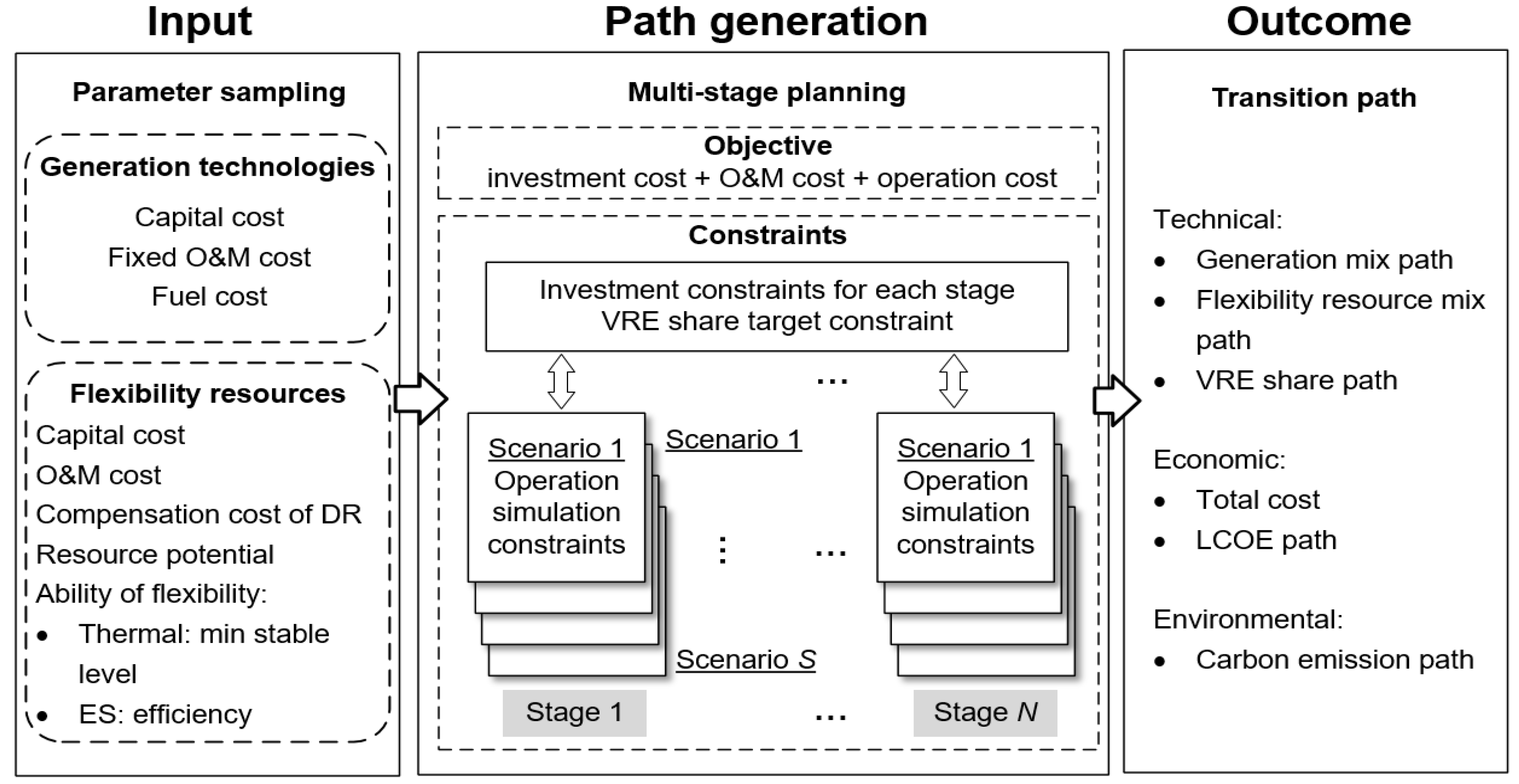
2.1. Path Generation under Multiple Uncertainties
2.1.1. Input
2.1.2. Path Generation
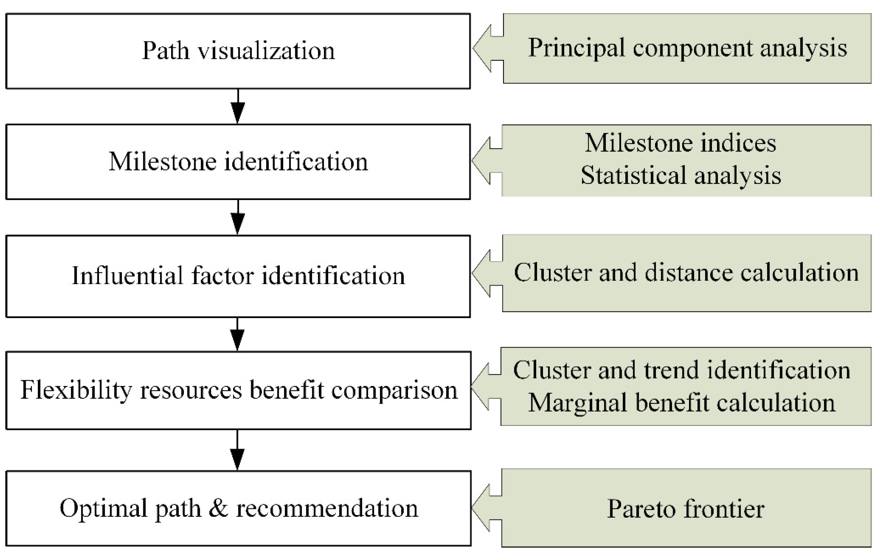
2.2. Data-Driven Path Analysis
2.2.1. PCA-Based Path Visualization and Milestone Identification
- Milestones for flexibility resources
- Flexibility requirement (FR):
- Marginal flexibility requirement (MFR)
- 2.
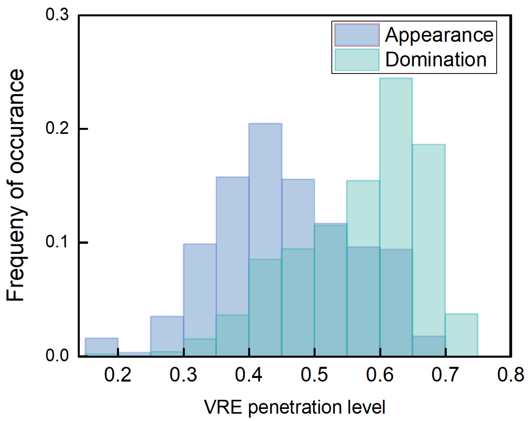
- Milestones for battery storage
- Milestone of battery appearance (MoA):
- Milestone of battery domination (MoD):
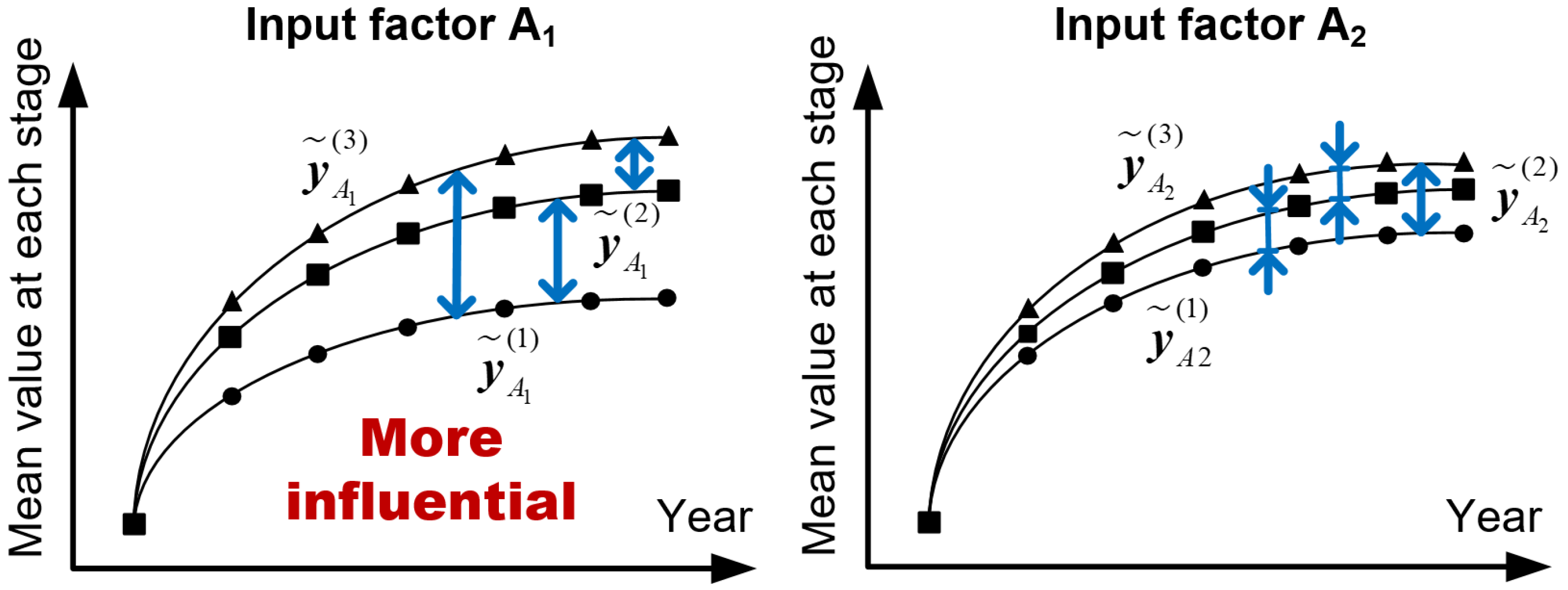
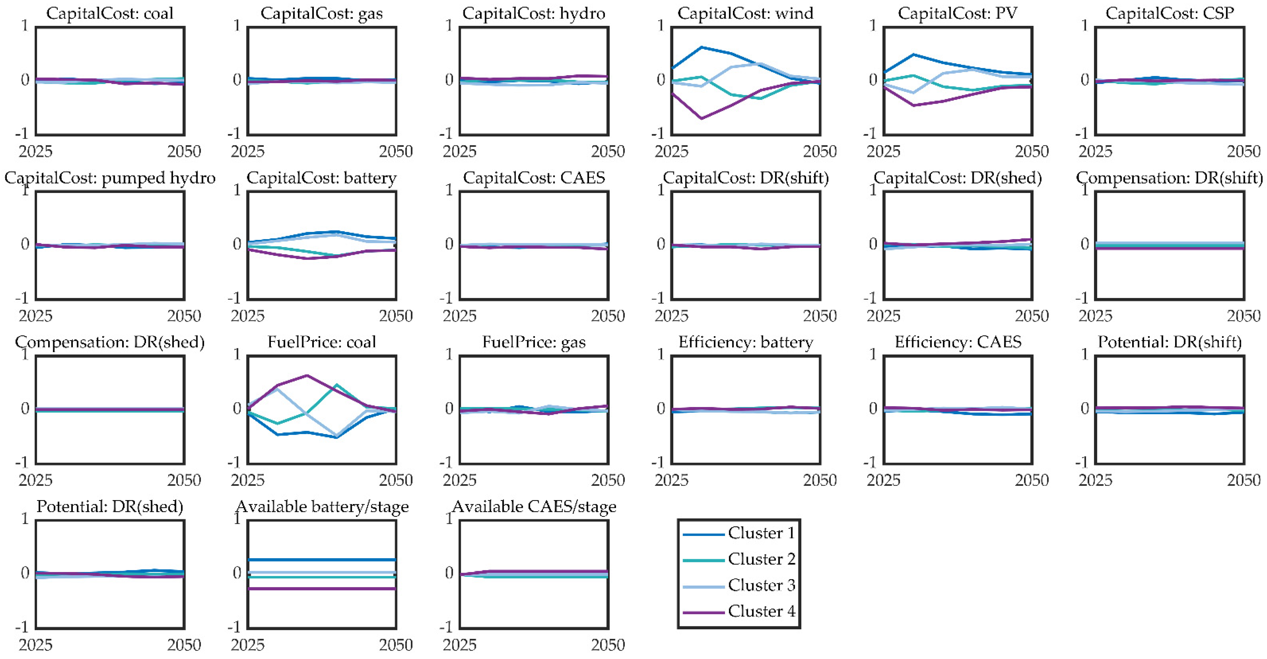
2.2.2. Cluster and Distance Calculation-Based Influential Factor Identification
- (1)
- Represent the ith input factor with yi. Since the factor value varies with development stages, yi is the time series composed of values at multiple stages:
- (2)
- Cluster the collection of paths into several groups. Assume that the number of groups is R. The ith input factor of the paths belonging to the rth group corresponds to a subspace within its uncertain space .
- (3)
- For each input factor yi, calculate the mean value at each stage over subspace to obtain time-series mean values:
- (4)
- Standardize as
- (5)
- Calculate the average distance among .
2.2.3. Cluster and Marginal Index-Based Flexibility Resources Benefit Comparison
- Cluster and Trend Identification
- 2.
- Marginal Benefit Calculation
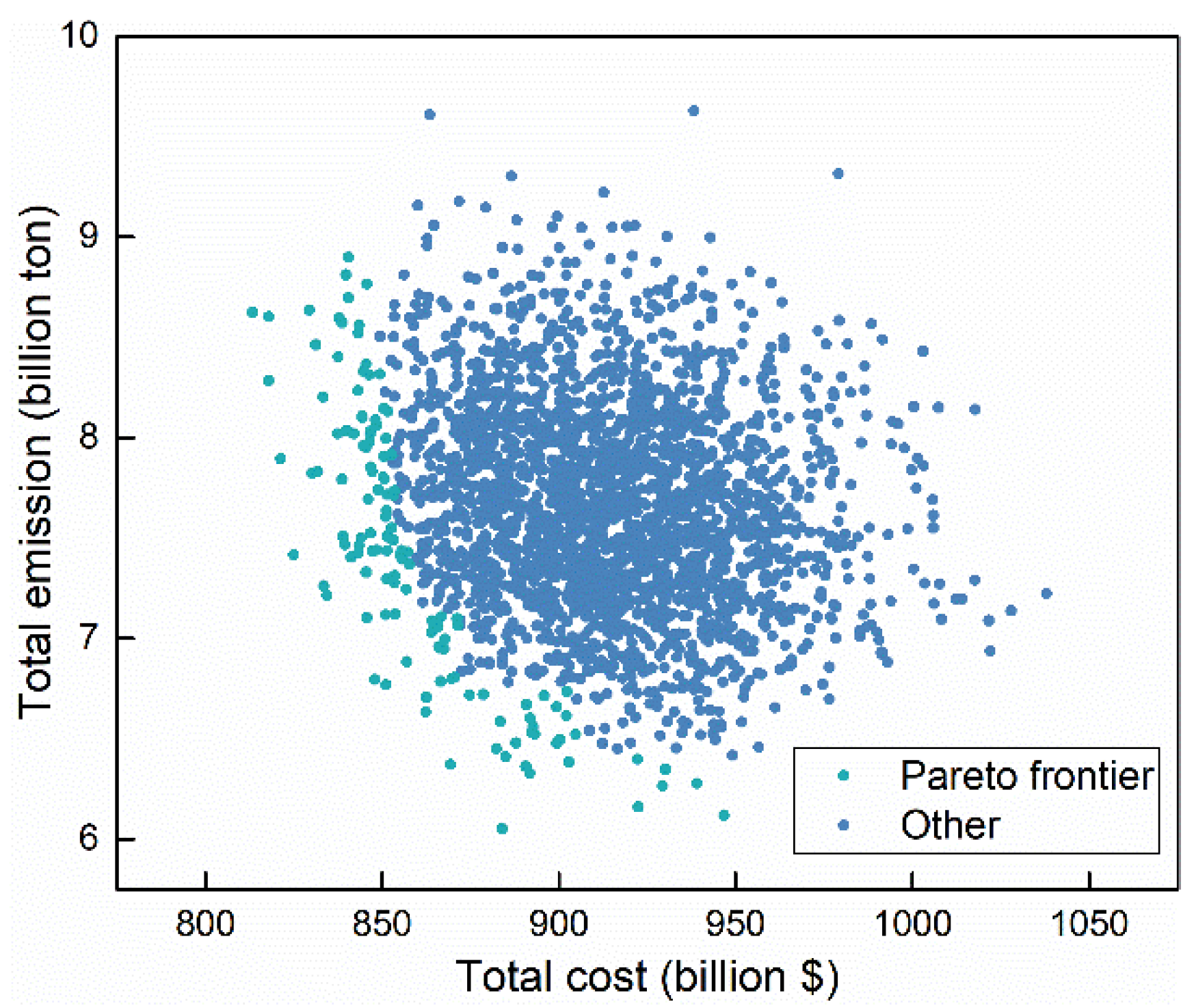
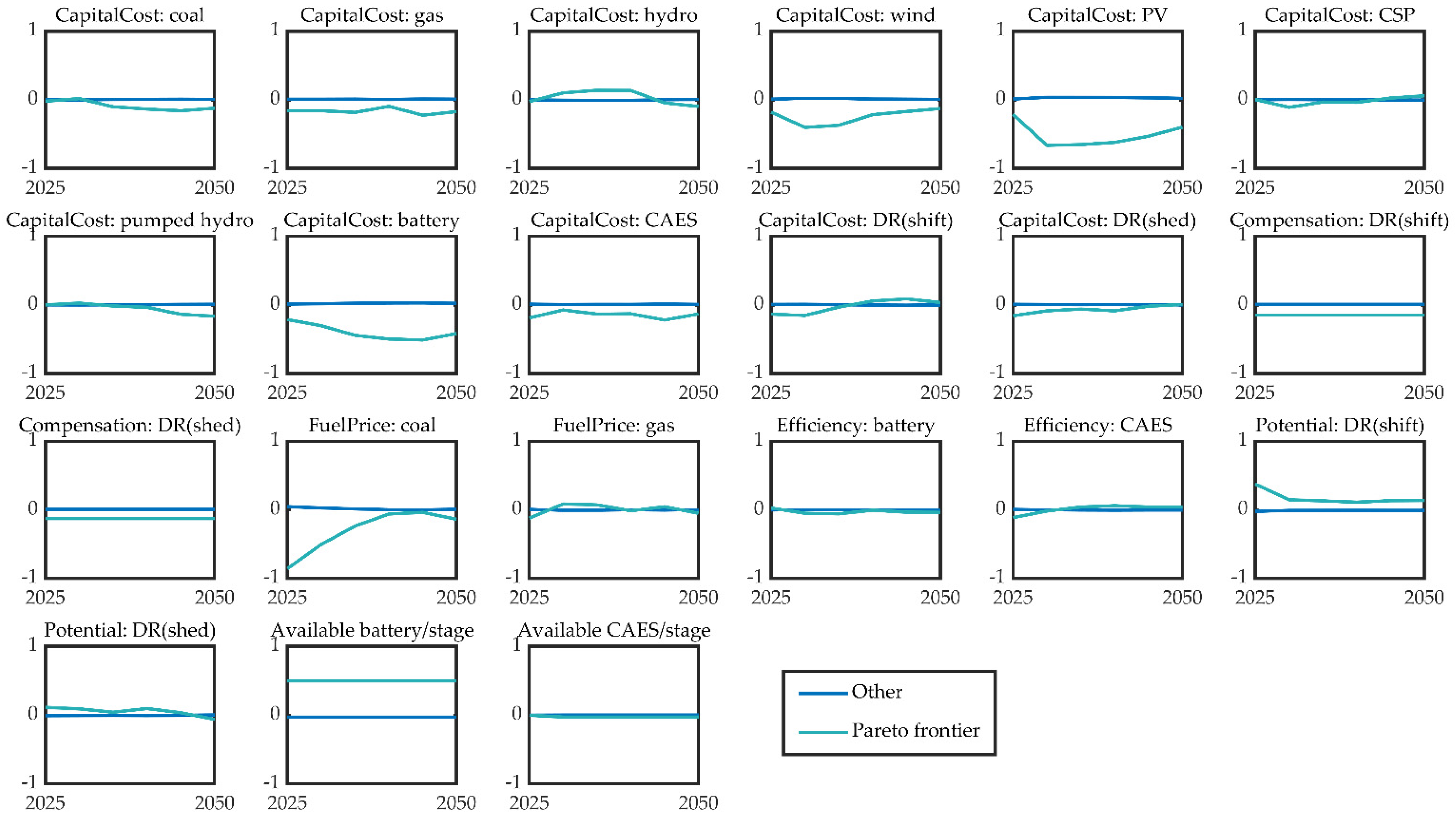
2.2.4. Pareto Frontier-Based Optimal Path Recommendation
3. Case Study
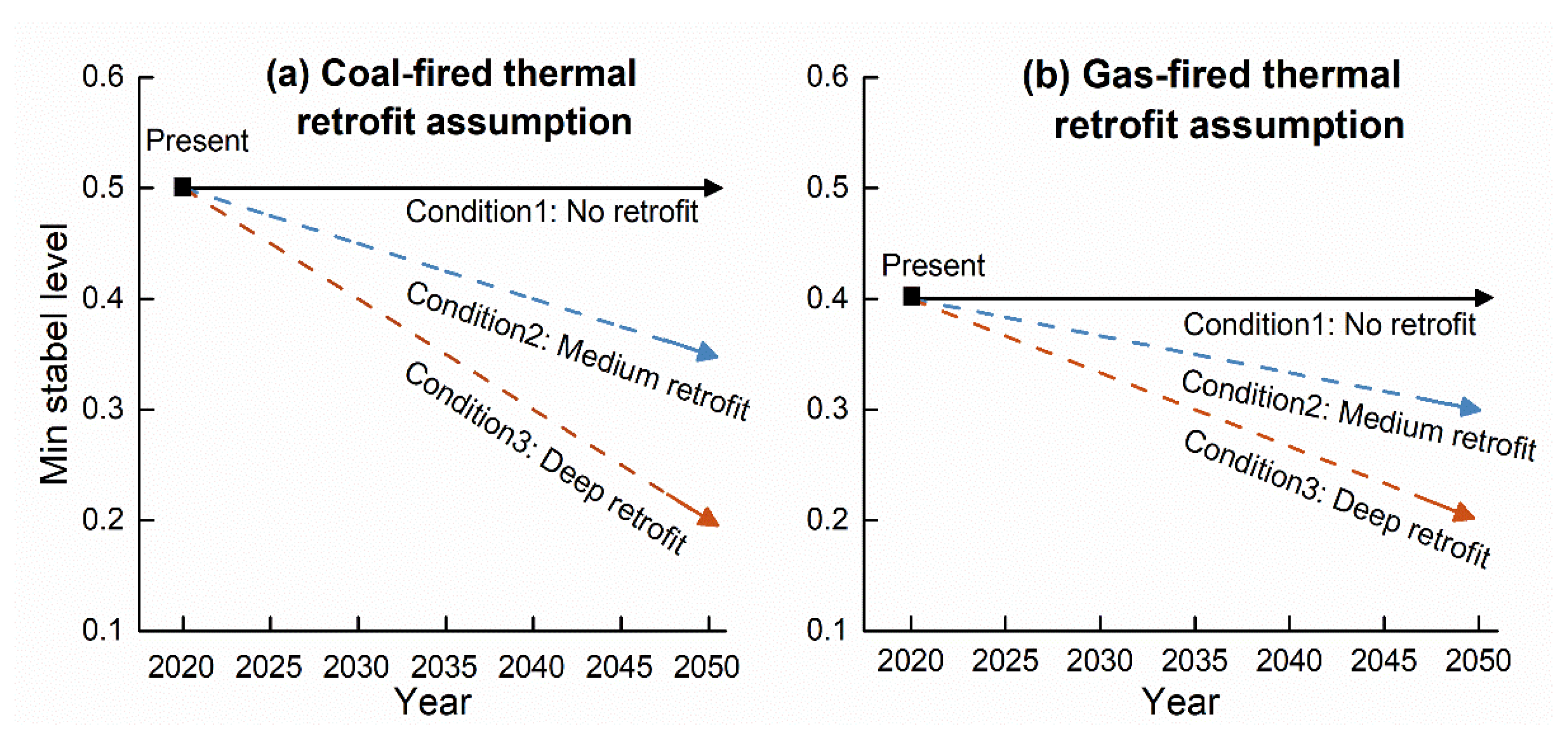
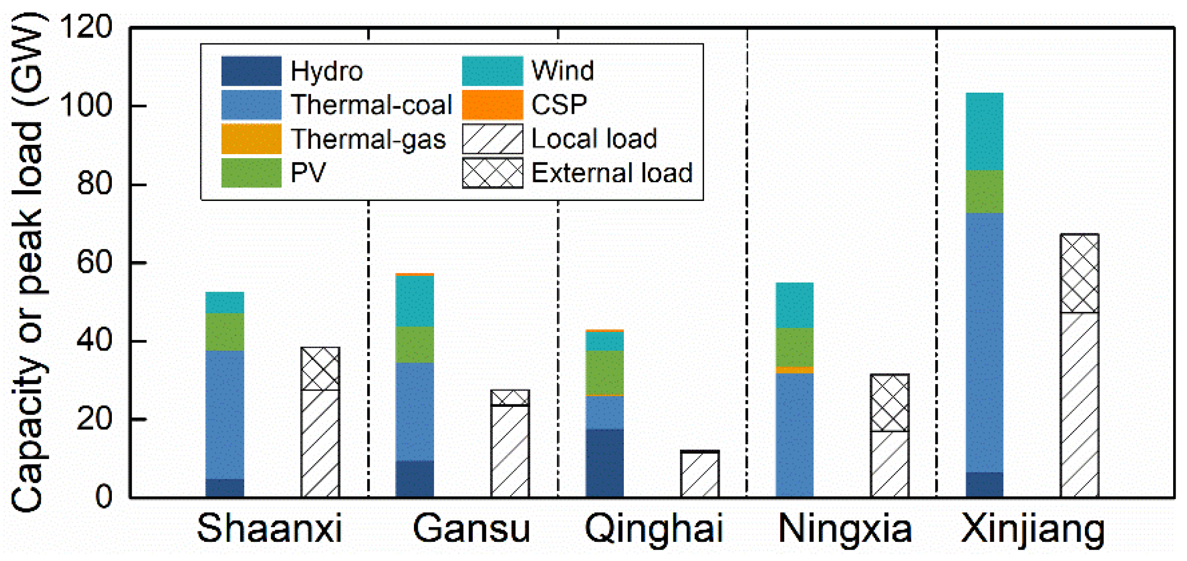
3.1. Input Data
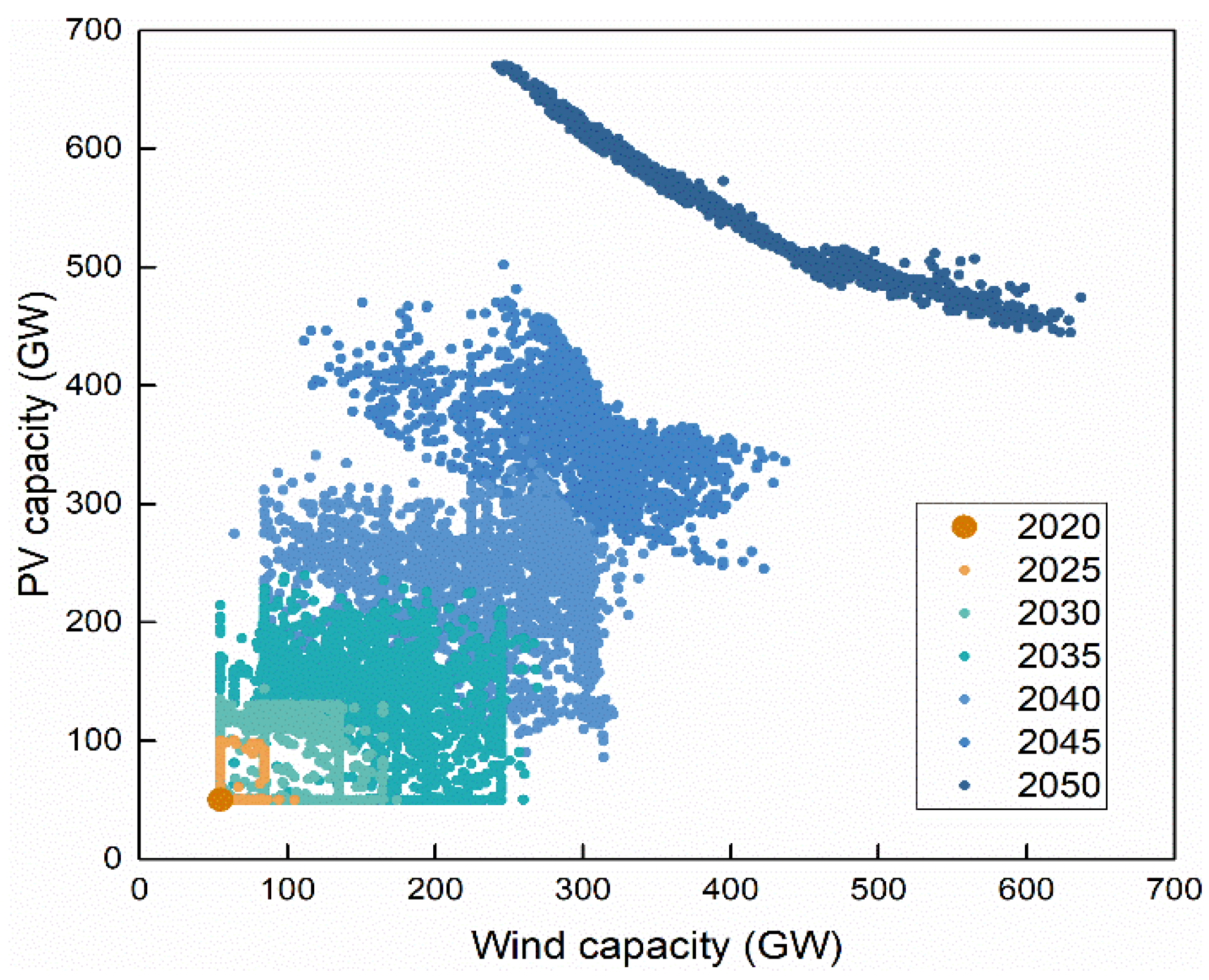
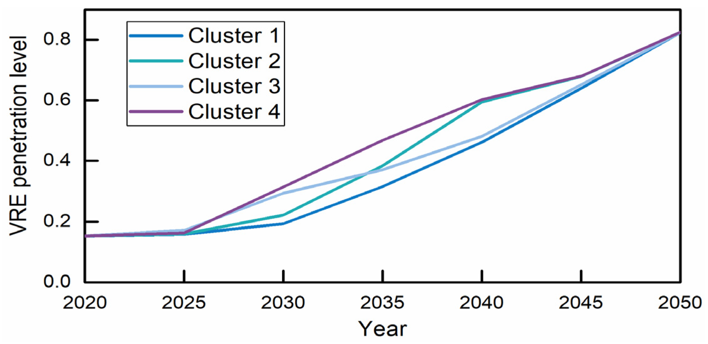
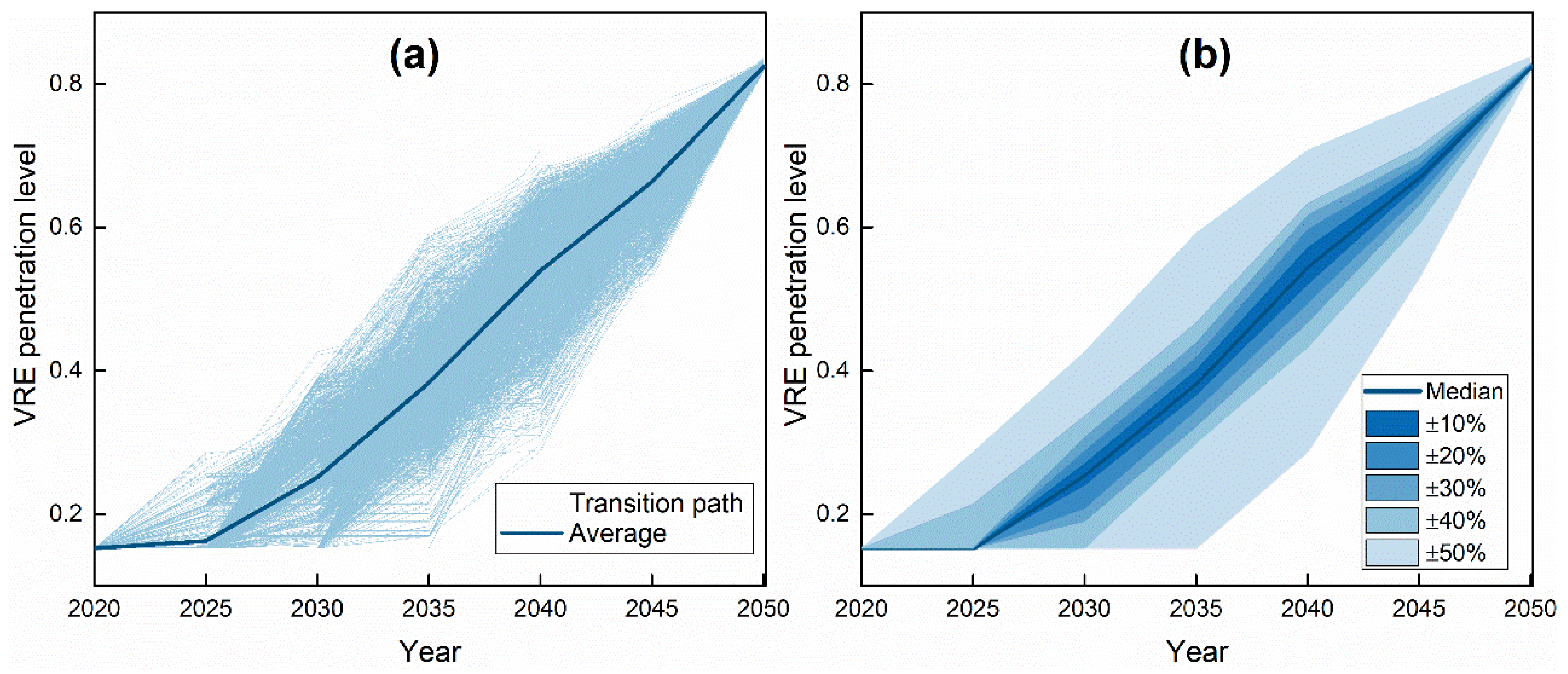
3.2. Path Visualization
3.3. Transition Milestones
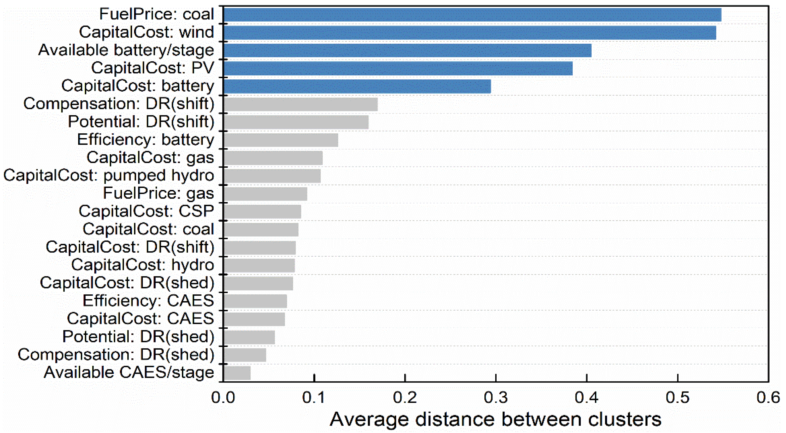
3.4. Key Influential Factors
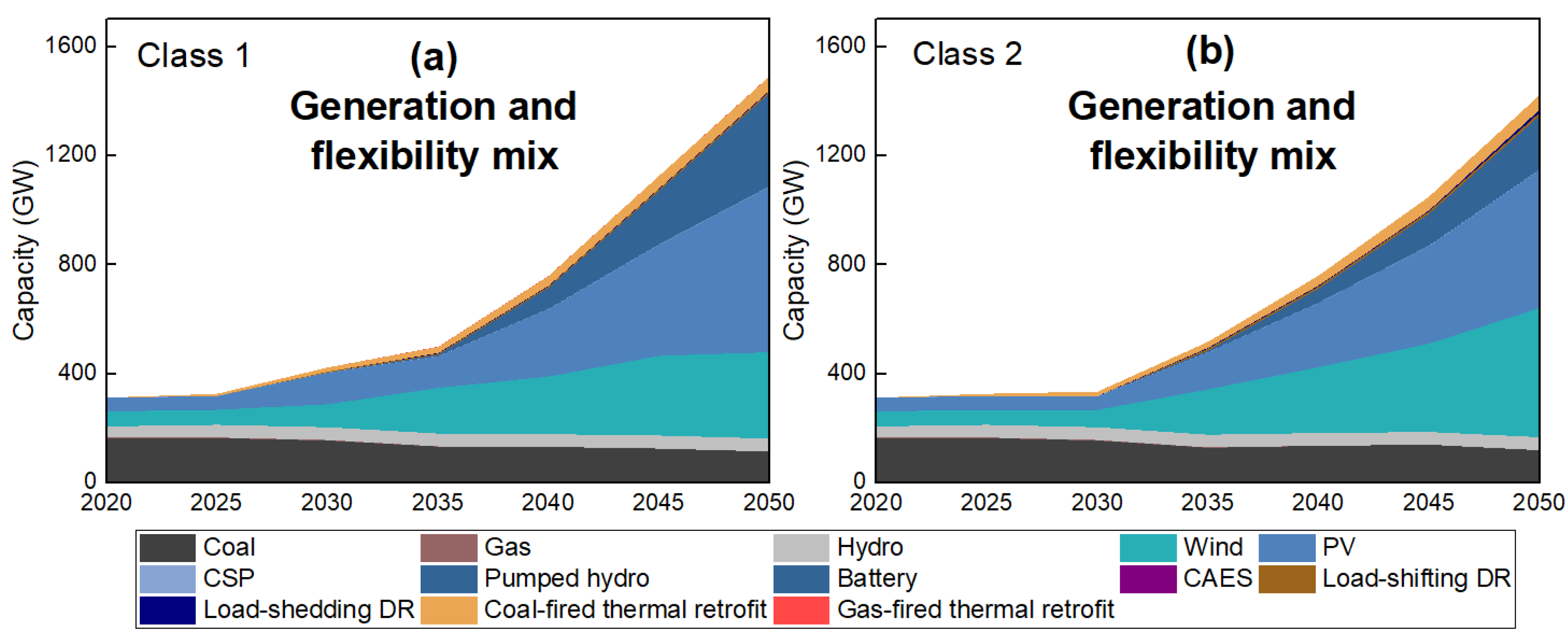
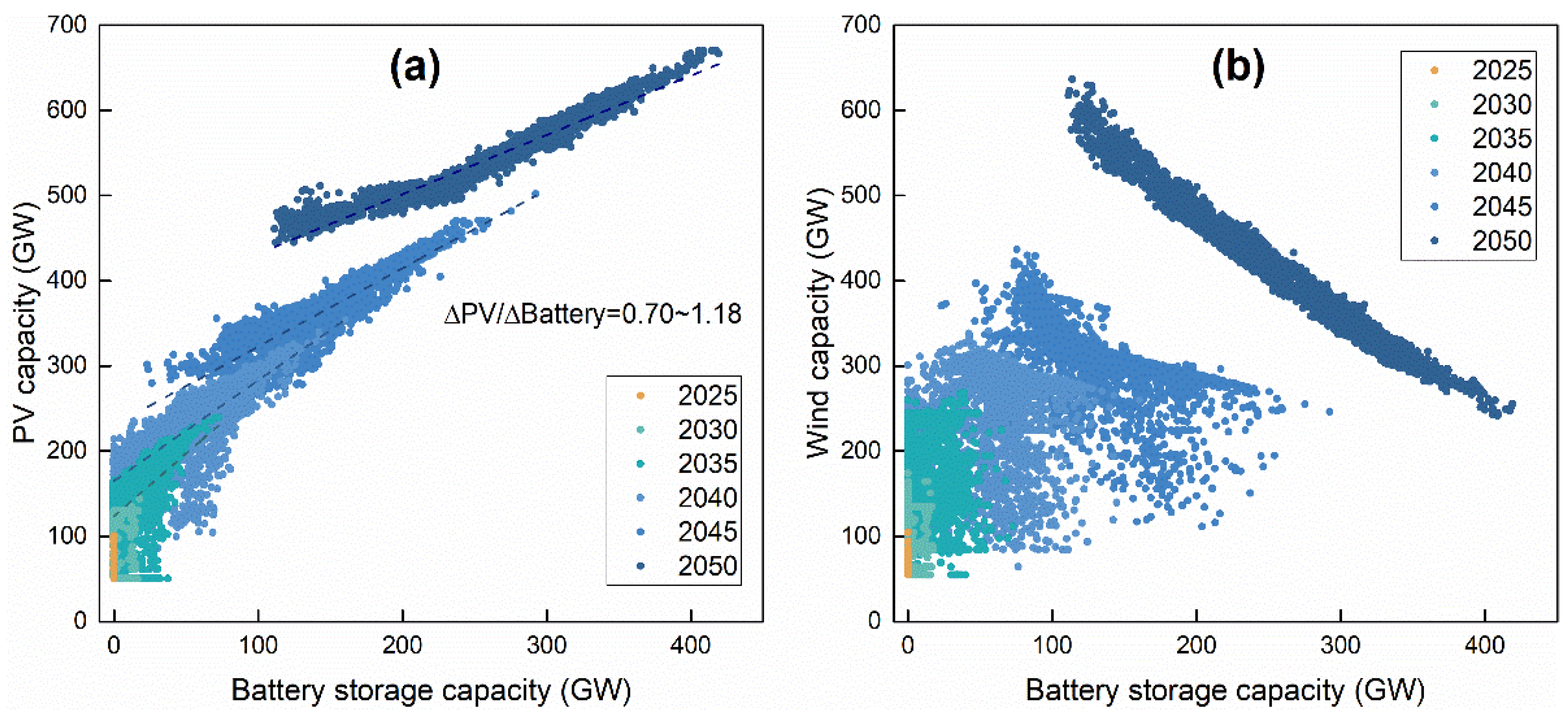
3.5. Benefit of Flexibility Resources
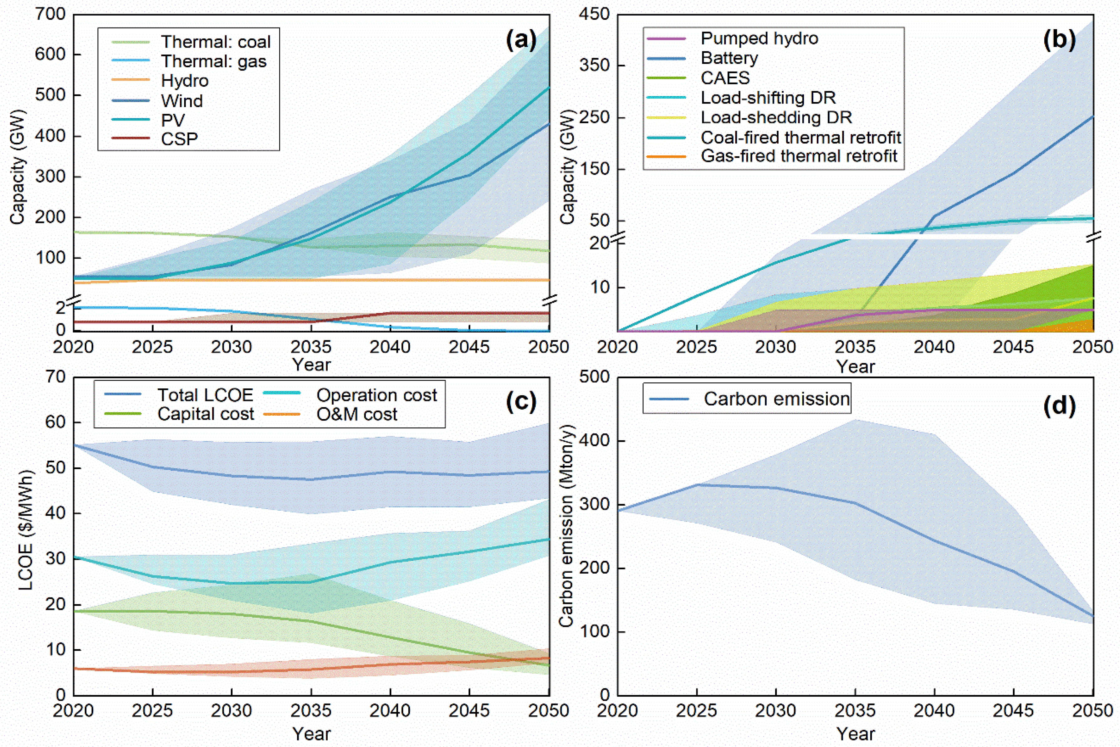
3.5.1. Technical Benefit
3.5.2. Economic Benefit
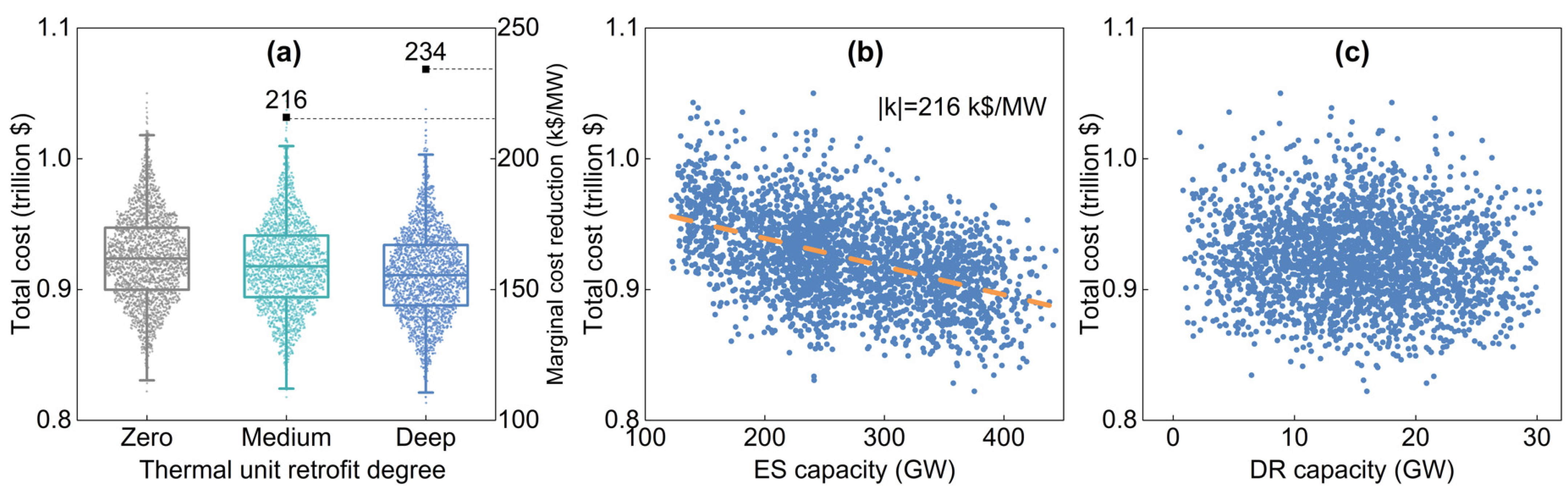
- (1)
- From the generation side, the total cost, including the investment, fixed O&M and variable operation costs for the whole transition, is compared across different thermal unit retrofit levels. The deeper the retrofit level is, the lower the total cost will be. We also calculate the marginal cost reduction as the cost reduction per retrofit capacity. For the medium and deep retrofits, the average marginal cost reductions over paths are 216 k$/MW and 234 k$/MW, respectively, which are close to each other.
- (2)
- From the storage side, the total cost shows a negative correlation with the storage capacity in 2050, which means that storage can also reduce the total cost. The slope of the linear fitting indicates that the average marginal cost reduction of the storage is 216 k$/MW, similar to that of the thermal retrofit.
- (3)
- From the demand side, there is no obvious correlation between the DR capacity in 2050 and the total cost, indicating that DR contributes little to the cost reduction. This is because, as shown in the table of the input parameters (Table A1), DR’s unit compensation cost obtained from a study in China [45] is overall higher than the coal price. Therefore, the cost of deploying DR may be more than the saved fuel cost, making it less economical. Note that the DR results apply only to the considered system and data. For other countries where DR is more economical, the results may be different.
3.5.3. Environmental Benefit
- (1)
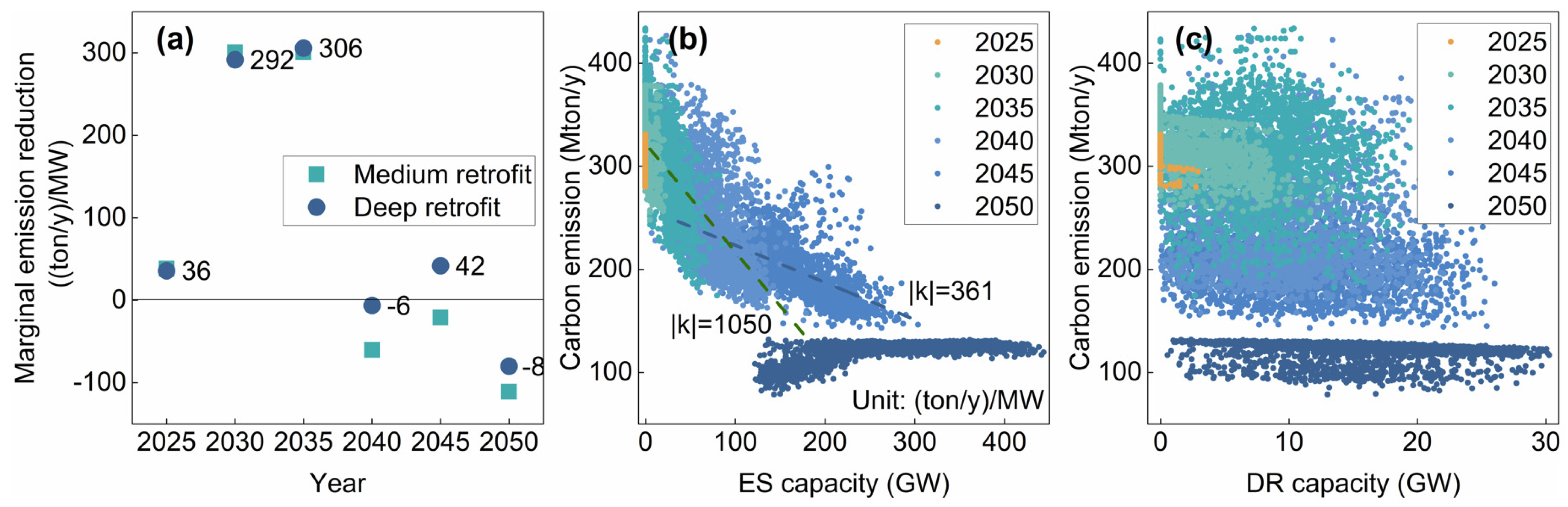
- From the generation side, the marginal emission reduction of the retrofit capacity is large in the early stages but negative in some stages. We investigate the reason by randomly checking a sample, as shown in Table A4. The table shows that the retrofit, which is cheaper than the battery in terms of investment cost, can replace part of the battery capacity under deep retrofit. This saves on the investment cost but may increase the operation cost because the thermal units are more likely to be committed to providing flexibility, which may result in more carbon emissions compared to the case with no retrofit but a large battery capacity.
- (2)
- From the storage side, the carbon emissions show a negative correlation with the storage capacity at most stages. In the last stage of 2050, emissions are relatively stable with different storage capacities because the VRE generation share in this stage is almost the same for all paths. From the slopes of the linear fitting, the marginal emission reduction of the storage is 361 (ton/y)/MW or above, higher than that of the thermal retrofit.
- (3)
- From the demand side, as discussed in Section 3.5.2, the allocation of DR may be influenced by complex factors, and thus, it does not show a clear relationship with the total cost or carbon emissions. We want to note again that the result may be different for other systems and data.
3.6. Optimal Paths and Recommendations
4. Conclusions
Author Contributions
Funding
Institutional Review Board Statement
Informed Consent Statement
Data Availability Statement
Acknowledgments
Conflicts of Interest
Appendix A. The Description of the Path Generation Model
- Objective Function
- 2.
- Constraints at the First Level
- 3.
- Constraints at the Second Level
Appendix B

| No. | Uncertain Parameters | Unit | 2025 | 2030 | 2035 | 2040 | 2045 | 2050 | Refs. | ||||||
|---|---|---|---|---|---|---|---|---|---|---|---|---|---|---|---|
| LB | UB | LB | UB | LB | UB | LB | UB | LB | UB | LB | UB | ||||
| 1 | Capital cost: coal-fired thermal | $/kW | 563 | 625 | 563 | 625 | 563 | 625 | 563 | 625 | 563 | 625 | 563 | 625 | [47] |
| 2 | Capital cost: gas-fired thermal | $/kW | 338 | 375 | 338 | 375 | 338 | 375 | 338 | 375 | 338 | 375 | 338 | 375 | [47] |
| 3 | Capital cost: hydro | $/kW | 1418 | 1424 | 1411 | 1424 | 1411 | 1424 | 1411 | 1424 | 1405 | 1424 | 1398 | 1424 | [42] |
| 4 | Capital cost: wind | $/kW | 1241 | 1385 | 1098 | 1385 | 1052 | 1379 | 1006 | 1372 | 980 | 1366 | 954 | 1359 | [42] |
| 5 | Capital cost: PV | $/kW | 876 | 1215 | 562 | 1241 | 503 | 1183 | 444 | 1124 | 405 | 1085 | 366 | 1045 | [42] |
| 6 | Capital cost: CSP | $/kW | 4998 | 6397 | 3502 | 6299 | 3280 | 6096 | 3058 | 5894 | 2960 | 5769 | 2862 | 5645 | [42] |
| 7 | Capital cost: pumped hydro | $/kW | 659 | 732 | 659 | 732 | 659 | 732 | 659 | 732 | 659 | 732 | 659 | 732 | [40] |
| 8 | Capital cost: battery storage | $/kW | 700 | 1320 | 496 | 1200 | 460 | 1160 | 400 | 1120 | 320 | 1100 | 300 | 1032 | [43] |
| 9 | Capital cost: CAES | $/kW | 3019 | 4523 | 2845 | 4471 | 2781 | 4371 | 2726 | 4284 | 2562 | 4026 | 2406 | 3781 | [40] |
| 10 | Capital cost: load-shifting DR | $/kW | 8 | 11 | 8 | 11 | 8 | 11 | 8 | 11 | 8 | 11 | 8 | 11 | [12] |
| 11 | Capital cost: load-shedding DR | $/kW | 10 | 14 | 10 | 14 | 10 | 14 | 10 | 14 | 10 | 14 | 10 | 14 | [12] |
| 12 | Compensation cost: load-shifting DR | $/MWh | 35 | 65 | 35 | 65 | 35 | 65 | 35 | 65 | 35 | 65 | 35 | 65 | [12] |
| 13 | Compensation cost: load-shedding DR | $/MWh | 45 | 84 | 45 | 84 | 45 | 84 | 45 | 84 | 45 | 84 | 45 | 84 | [12] |
| 14 | Fuel price: coal | $/MWh | 20.4 | 30.6 | 22.4 | 33.5 | 24.8 | 37.2 | 27.0 | 40.5 | 27.0 | 40.5 | 27.0 | 40.5 | [40] |
| 15 | Fuel price: gas | $/MWh | 54.1 | 81.1 | 58.9 | 88.4 | 65.1 | 97.6 | 72.5 | 108.7 | 72.5 | 108.7 | 72.5 | 108.7 | [40] |
| 16 | Efficiency: battery storage | - | 90.0 | 95.0 | 90.0 | 95.0 | 90.0 | 95.0 | 90.0 | 95.0 | 90.0 | 95.0 | 90.0 | 95.0 | [40] |
| 17 | Efficiency: CAES | - | 59.0 | 70.0 | 59.0 | 70.0 | 59.0 | 70.0 | 59.0 | 70.0 | 59.0 | 70.0 | 59.0 | 70.0 | [40] |
| 18 | Potential: load-shifting DR | - | 0.00 | 0.05 | 0.00 | 0.05 | 0.00 | 0.05 | 0.00 | 0.05 | 0.00 | 0.05 | 0.00 | 0.05 | |
| 19 | Potential: load-shedding DR | - | 0.00 | 0.05 | 0.00 | 0.05 | 0.00 | 0.05 | 0.00 | 0.05 | 0.00 | 0.05 | 0.00 | 0.05 | |
| 20 | Available battery investment for each stage | - | Assume linear increase with time, and the increase ratio are uncertain | ||||||||||||
| 21 | Available CAES investment for each stage | - | Assume linear increase with time, and the increase ratio are uncertain | ||||||||||||
| Stage | 2025 | 2030 | 2035 | 2040 | 2045 | 2050 | ||||||
|---|---|---|---|---|---|---|---|---|---|---|---|---|
| Coal | 0.00 | 0.00 | 0.00 | 0.00 | −0.02 | 0.06 | 0.04 | −0.14 | −0.10 | 0.12 | −0.07 | 0.01 |
| Gas | 0.00 | 0.00 | 0.00 | 0.00 | 0.00 | 0.00 | 0.00 | 0.00 | 0.00 | 0.00 | 0.00 | 0.00 |
| Hydro | 0.00 | 0.00 | 0.00 | 0.00 | 0.00 | 0.00 | 0.00 | 0.00 | 0.00 | 0.00 | 0.00 | 0.00 |
| Wind | 1.00 | −0.08 | 0.40 | 0.92 | 0.94 | −0.32 | −0.99 | 0.08 | −0.53 | −0.84 | −0.70 | 0.29 |
| PV | 0.08 | 1.00 | −0.92 | 0.40 | −0.34 | −0.91 | 0.12 | 0.86 | 0.60 | −0.43 | 0.41 | 0.90 |
| CSP | 0.00 | 0.00 | 0.00 | 0.00 | 0.00 | 0.00 | 0.00 | 0.00 | 0.00 | 0.00 | 0.00 | 0.00 |
| Pumped hydro | 0.00 | 0.00 | −0.01 | 0.01 | 0.00 | −0.03 | 0.00 | 0.01 | 0.00 | 0.00 | 0.00 | 0.00 |
| Battery | 0.00 | 0.00 | −0.01 | 0.01 | 0.01 | −0.23 | −0.04 | 0.48 | 0.59 | −0.30 | 0.58 | −0.28 |
| CAES | 0.00 | 0.00 | 0.00 | 0.00 | 0.00 | 0.00 | 0.00 | 0.00 | −0.01 | −0.01 | −0.01 | 0.11 |
| Load-shifting DR | 0.00 | 0.02 | −0.03 | 0.04 | 0.01 | −0.02 | 0.00 | 0.00 | 0.00 | 0.00 | 0.00 | 0.08 |
| Load-shedding DR | 0.00 | 0.00 | 0.00 | 0.00 | 0.00 | 0.03 | 0.00 | −0.01 | 0.00 | 0.01 | 0.00 | 0.01 |
| Coal-fired thermal retrofit | 0.00 | 0.00 | 0.00 | 0.00 | 0.00 | 0.01 | 0.01 | −0.03 | −0.03 | 0.03 | −0.02 | 0.00 |
| Gas-fired thermal retrofit | 0.00 | 0.00 | 0.00 | 0.00 | 0.00 | 0.00 | 0.00 | 0.00 | 0.00 | 0.00 | 0.00 | 0.00 |
| Cumulative explanation | 1.00 | 0.99 | 0.96 | 0.95 | 0.96 | 0.99 | ||||||
| Aspect of Transition Path | Technical | Economic | Environmental | |
|---|---|---|---|---|
| Generation Mix | Flexiblility Mix | LCOE | Carbon Emission | |
| CapitalCost: coal | 0.03 | 0.09 | 0.06 | 0.07 |
| CapitalCost: gas | 0.11 | 0.10 | 0.09 | 0.05 |
| CapitalCost: hydro | 0.10 | 0.08 | 0.09 | 0.08 |
| CapitalCost: wind | 0.17 | 0.11 | 0.24 | 0.53 |
| CapitalCost: PV | 0.36 | 0.37 | 0.19 | 0.32 |
| CapitalCost: CSP | 0.15 | 0.13 | 0.14 | 0.08 |
| CapitalCost: pumped hydro | 0.09 | 0.04 | 0.06 | 0.09 |
| CapitalCost: battery | 0.46 | 0.55 | 0.22 | 0.25 |
| CapitalCost: CAES | 0.08 | 0.08 | 0.14 | 0.07 |
| CapitalCost: DR(shift) | 0.07 | 0.10 | 0.08 | 0.08 |
| CapitalCost: DR(shed) | 0.05 | 0.15 | 0.11 | 0.12 |
| Compensation: DR(shift) | 0.09 | 0.08 | 0.03 | 0.03 |
| Compensation: DR(shed) | 0.06 | 0.06 | 0.16 | 0.05 |
| FuelPrice: coal | 0.21 | 0.18 | 0.96 | 0.56 |
| FuelPrice: gas | 0.07 | 0.06 | 0.10 | 0.08 |
| Efficiency: battery | 0.05 | 0.06 | 0.10 | 0.07 |
| Efficiency: CAES | 0.06 | 0.08 | 0.06 | 0.06 |
| Potential: DR(shift) | 0.11 | 0.18 | 0.10 | 0.10 |
| Potential: DR(shed) | 0.11 | 0.10 | 0.09 | 0.08 |
| Available battery/stage | 1.24 | 1.39 | 0.12 | 0.31 |
| Available CAES/stage | 0.06 | 0.11 | 0.03 | 0.06 |
| Retrofit Degree | No Retrofit | Deep Retrofit | |
|---|---|---|---|
| Capacity in 2050 (MW) | Coal-fired thermal | 106,329 | 111,855 |
| Gas-fired thermal | 6 | 6 | |
| Hydro | 46,920 | 46,920 | |
| Wind | 328,872 | 346,541 | |
| PV | 594,441 | 583,673 | |
| CSP | 1600 | 1600 | |
| Pumped hydro | 5000 | 5000 | |
| Battery | 370,102 | 323,906 | |
| CAES | 0 | 0 | |
| Load-shifting DR | 1087 | 1087 | |
| Load-shedding DR | 11,506 | 11,506 | |
| Coal-fired thermal retrofit | 0 | 51,539 | |
| Gas-fired thermal retrofit | 0 | 176 | |
| Cost (billion $) | Investment cost | 561 | 548 |
| Fixed O&M cost | 10 | 10 | |
| Variable operation cost | 320 | 328 | |
| Total cost | 891 | 886 | |
References
- Mai, T.; Sandor, D.; Wiser, R.; Schneider, T. Renewable Electricity Futures Study. Executive Summary; National Renewable Energy Lab. (NREL): Golden, CO, USA, 2012. [Google Scholar]
- European Climate Foundation. Roadmap 2050. Available online: https://www.roadmap2050.eu/reports (accessed on 5 September 2021).
- Energy Research Institute and National Development and Reform Commission. China 2050 High Renewable Energy Penetration Scenario and Roadmap Study; Energy Research Institute and National Development and Reform Commission: Beijing, China, 2015. [Google Scholar]
- Mohandes, B.; Moursi, M.S.E.; Hatziargyriou, N.; Khatib, S.E. A Review of Power System Flexibility With High Penetration of Renewables. IEEE Trans. Power Syst. 2019, 34, 3140–3155. [Google Scholar] [CrossRef]
- Alizadeh, M.; Moghaddam, M.P.; Amjady, N.; Siano, P.; Sheikh-El-Eslami, M. Flexibility in future power systems with high renewable penetration: A review. Renew. Sustain. Energy Rev. 2016, 57, 1186–1193. [Google Scholar] [CrossRef]
- International Energy Agency (IEA). Status of Power System Transformation 2019; IEA: Paris, France, 2019. [Google Scholar]
- International Energy Agency (IEA). World Energy Outlook 2018; IEA: Paris, France, 2018. [Google Scholar]
- International Energy Agency (IEA). China Power System Transformation-Assessing the Benefit of Optimised Operations and Advanced Flexibility Options; IEA: Paris, France, 2019. [Google Scholar]
- International Renewable Energy Agency (IRENA). Power System Flexibility for the Energy Transition; IRENA: Abu Dhabi, United Arab Emirates, 2018. [Google Scholar]
- Hansen, K.; Breyer, C.; Lund, H. Status and perspectives on 100% renewable energy systems. Energy 2019, 175, 471–480. [Google Scholar] [CrossRef]
- IRENA. Innovation Landscape for a Renewable-Powered Future; IRENA: Abu Dhabi, United Arab Emirates, 2019. [Google Scholar]
- Li, H.; Lu, Z.; Qiao, Y.; Zhang, B.; Lin, Y. The flexibility test system for studies of variable renewable energy resources. IEEE Trans. Power Syst. 2021, 36, 1526–1536. [Google Scholar] [CrossRef]
- Venkataraman, S.; Jordan, G.; O’Connor, M.; Kumar, N.; Lefton, S.; Lew, D.; Brinkman, G.; Palchak, D.; Cochran, J. Cost-Benefit Analysis of Flexibility Retrofits for Coal and Gas-Fueled Power Plants: August 2012–December 2013; National Renewable Energy Lab.(NREL): Golden, CO, USA, 2013. [Google Scholar]
- Connolly, D.; Lund, H.; Mathiesen, B.V.; Leahy, M. The first step towards a 100% renewable energy-system for Ireland. Appl. Energy 2011, 88, 502–507. [Google Scholar] [CrossRef]
- Dominković, D.F.; Bačeković, I.; Ćosić, B.; Krajačić, G.; Pukšec, T.; Duić, N.; Markovska, N. Zero carbon energy system of South East Europe in 2050. Appl. Energy 2016, 184, 1517–1528. [Google Scholar] [CrossRef] [Green Version]
- Mathiesen, B.V.; Lund, H.; Karlsson, K. 100% Renewable energy systems, climate mitigation and economic growth. Appl. Energy 2011, 88, 488–501. [Google Scholar] [CrossRef]
- Panos, E.; Kober, T.; Wokaun, A. Long term evaluation of electric storage technologies vs alternative flexibility options for the Swiss energy system. Appl. Energy 2019, 252, 113470. [Google Scholar] [CrossRef]
- Morgan, M.G.; Keith, D.W. Improving the way we think about projecting future energy use and emissions of carbon dioxide. Clim. Chang. 2008, 90, 189–215. [Google Scholar] [CrossRef]
- Syri, S.; Lehtilä, A.; Ekholm, T.; Savolainen, I.; Holttinen, H.; Peltola, E. Global energy and emissions scenarios for effective climate change mitigation—Deterministic and stochastic scenarios with the TIAM model. Int. J. Greenh. Gas Control 2008, 2, 274–285. [Google Scholar] [CrossRef]
- Bistline, J.E.; Weyant, J.P. Electric sector investments under technological and policy-related uncertainties: A stochastic programming approach. Clim. Chang. 2013, 121, 143–160. [Google Scholar] [CrossRef]
- Usher, W.; Strachan, N. Critical mid-term uncertainties in long-term decarbonisation pathways. Energy Policy 2012, 41, 433–444. [Google Scholar] [CrossRef] [Green Version]
- Labriet, M.; Nicolas, C.; Tchung-Ming, S.; Kanudia, A.; Loulou, R. Energy decisions in an uncertain climate and technology outlook: How stochastic and robust methodologies can assist policy-makers. In Informing Energy and Climate Policies Using Energy Systems Models; Springer: Berlin/Heidelberg, Germany, 2015; pp. 69–91. [Google Scholar]
- Babonneau, F.; Kanudia, A.; Labriet, M.; Loulou, R.; Vial, J.-P. Energy security: A robust optimization approach to design a robust European energy supply via TIAM-WORLD. Environ. Modeling Assess. 2012, 17, 19–37. [Google Scholar] [CrossRef]
- Saltelli, A.; Ratto, M.; Andres, T.; Campolongo, F.; Cariboni, J.; Gatelli, D.; Saisana, M.; Tarantola, S. Global Sensitivity Analysis: The Primer; John Wiley & Sons: Hoboken, NJ, USA, 2008. [Google Scholar]
- Kwakkel, J.H.; Pruyt, E. Exploratory modeling and analysis, an approach for model-based foresight under deep uncertainty. Technol. Forecast. Soc. Chang. 2013, 80, 419–431. [Google Scholar] [CrossRef]
- Bishop, C.M. Pattern Recognition and Machine Learning; Springer: Berlin/Heidelberg, Germany, 2006. [Google Scholar]
- Pye, S.; Sabio, N.; Strachan, N. An integrated systematic analysis of uncertainties in UK energy transition pathways. Energy Policy 2015, 87, 673–684. [Google Scholar] [CrossRef] [Green Version]
- Moallemi, E.A.; de Haan, F.; Kwakkel, J.; Aye, L. Narrative-informed exploratory analysis of energy transition pathways: A case study of India’s electricity sector. Energy Policy 2017, 110, 271–287. [Google Scholar] [CrossRef]
- Yue, X.; Patankar, N.; Decarolis, J.; Chiodi, A.; Rogan, F.; Deane, J.P.; O’Gallachoir, B. Least cost energy system pathways towards 100% renewable energy in Ireland by 2050. Energy 2020, 207, 118264. [Google Scholar] [CrossRef]
- Bosetti, V.; Marangoni, G.; Borgonovo, E.; Diaz Anadon, L.; Barron, R.; McJeon, H.C.; Politis, S.; Friley, P. Sensitivity to energy technology costs: A multi-model comparison analysis. Energy Policy 2015, 80, 244–263. [Google Scholar] [CrossRef] [Green Version]
- Zsiborács, H.; Baranyai, N.H.; Vincze, A.; Zentkó, L.; Birkner, Z.; Máté, K.; Pintér, G. Intermittent renewable energy sources: The role of energy storage in the European power system of 2040. Electronics 2019, 8, 729. [Google Scholar] [CrossRef] [Green Version]
- Sadiqa, A.; Gulagi, A.; Breyer, C. Energy transition roadmap towards 100% renewable energy and role of storage technologies for Pakistan by 2050. Energy 2018, 147, 518–533. [Google Scholar] [CrossRef]
- Cebulla, F.; Naegler, T.; Pohl, M. Electrical energy storage in highly renewable European energy systems: Capacity requirements, spatial distribution, and storage dispatch. J. Energy Storage 2017, 14, 211–223. [Google Scholar] [CrossRef] [Green Version]
- Liu, H.; Brown, T.; Andresen, G.B.; Schlachtberger, D.P.; Greiner, M. The role of hydro power, storage and transmission in the decarbonization of the Chinese power system. Appl. Energy 2019, 239, 1308–1321. [Google Scholar] [CrossRef] [Green Version]
- China National Renewable Energy Center (CNREC). China Renewable Energy Outlook 2018; CNREC: Beijing, China, 2018. [Google Scholar]
- Mongird, K.; Fotedar, V.; Viswanathan, V.; Koritarov2, V.; Balducci, P.; Hadjerioua, B.; Alam, J. Energy Storage Technology and Cost Characterization Report; Pacific Northwest National Lab.(PNNL): Richland, WA, USA, 2019. [Google Scholar]
- Gils, H.C. Assessment of the theoretical demand response potential in Europe. Energy 2014, 67, 1–18. [Google Scholar] [CrossRef]
- Yue, X.; Pye, S.; DeCarolis, J.; Li, F.G.N.; Rogan, F.; Gallachóir, B.Ó. A review of approaches to uncertainty assessment in energy system optimization models. Energy Strategy Rev. 2018, 21, 204–217. [Google Scholar] [CrossRef]
- Chen, X.Y.; Lv, J.J.; McElroy, M.B.; Han, X.N.; Nielsen, C.P.; Wen, J.Y. Power system capacity expansion under higher penetration of renewables considering flexibility constraints and low carbon policies. IEEE Trans. Power Syst. 2018, 33, 6240–6253. [Google Scholar] [CrossRef]
- Bogdanov, D.; Farfan, J.; Sadovskaia, K.; Aghahosseini, A.; Child, M.; Gulagi, A.; Oyewo, A.S.; de Souza Noel Simas Barbosa, L.; Breyer, C. Radical transformation pathway towards sustainable electricity via evolutionary steps. Nat. Commun. 2019, 10, 1077. [Google Scholar] [CrossRef] [Green Version]
- Moallemi, E.A.; Köhler, J. Coping with uncertainties of sustainability transitions using exploratory modelling: The case of the MATISSE model and the UK’s mobility sector. Environ. Innov. Soc. Transit. 2019, 33, 61–83. [Google Scholar] [CrossRef]
- Tsiropoulos, I.; Tarvydas, D.; Zucker, A. Cost Development of Low Carbon Energy Technologies-Scenario-Based Cost Trajectories to 2050, 2017 ed.; European Union: Maastricht, The Netherlands, 2018. [Google Scholar]
- Cole, W.J.; Frazier, A. Cost Projections for Utility-Scale Battery Storage; National Renewable Energy Lab. (NREL): Golden, CO, USA, 2019. [Google Scholar]
- Global Energy Interconnection Development and Cooperation Organization (GEIDCO). Study on China’s 14th Five-Year Development Plan for the Power Sector; GEIDCO: Bangkok, Thailand, 2020. [Google Scholar]
- Zhang, N.; Dai, H.; Hu, Z. A Source-Grid-Load Coordinated Planning Model Considering System Flexibility Constraints and Demand Response. Electr. Power 2019, 52, 61–69. [Google Scholar] [CrossRef]
- Du, E.; Zhang, N.; Hodge, B.-M.; Wang, Q.; Kang, C.; Kroposki, B.; Xia, Q. The role of concentrating solar power toward high renewable energy penetrated power systems. IEEE Trans. Power Syst. 2018, 33, 6630–6641. [Google Scholar] [CrossRef]
- China Electric Power Planning & Engineering Institute. Report on China’s Electric Power Development 2020; People’s Daily Press: Beijing, China, 2021. [Google Scholar]


Publisher’s Note: MDPI stays neutral with regard to jurisdictional claims in published maps and institutional affiliations. |
© 2022 by the authors. Licensee MDPI, Basel, Switzerland. This article is an open access article distributed under the terms and conditions of the Creative Commons Attribution (CC BY) license (https://creativecommons.org/licenses/by/4.0/).
Share and Cite
Li, H.; Qiao, Y.; Lu, Z.; Zhang, B. Power System Transition with Multiple Flexibility Resources: A Data-Driven Approach. Sustainability 2022, 14, 2656. https://doi.org/10.3390/su14052656
Li H, Qiao Y, Lu Z, Zhang B. Power System Transition with Multiple Flexibility Resources: A Data-Driven Approach. Sustainability. 2022; 14(5):2656. https://doi.org/10.3390/su14052656
Chicago/Turabian StyleLi, Hao, Ying Qiao, Zongxiang Lu, and Baosen Zhang. 2022. "Power System Transition with Multiple Flexibility Resources: A Data-Driven Approach" Sustainability 14, no. 5: 2656. https://doi.org/10.3390/su14052656
APA StyleLi, H., Qiao, Y., Lu, Z., & Zhang, B. (2022). Power System Transition with Multiple Flexibility Resources: A Data-Driven Approach. Sustainability, 14(5), 2656. https://doi.org/10.3390/su14052656