
A Cost-Effective Solution for Non-Convex Economic Load Dispatch Problems in Power Systems Using Slime Mould Algorithm

 ,
,  ,
,  and
and
Abstract
:1. Introduction
- The slime mould algorithm is implemented as it has great global search capability.
- The SM algorithm is used to solve a non-convex and cost-effective load dispatch problem (ELD) in an electric power system.
- The efficiency of the algorithm is tested on standard IEEE test systems.
- The method is evaluated on nine different test systems with and without valve-point loading effects.
2. Literature Survey
3. Mathematical Formulation for Single-Area Economic Load Dispatch
3.1. Single-Area Economic Load Dispatch
3.1.1. Power Balance Constraint
3.1.2. Generator Limit Constraint
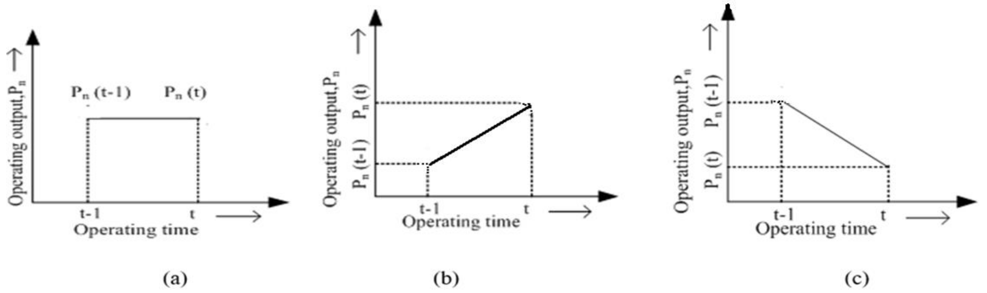
3.1.3. Ramp Rate Limits
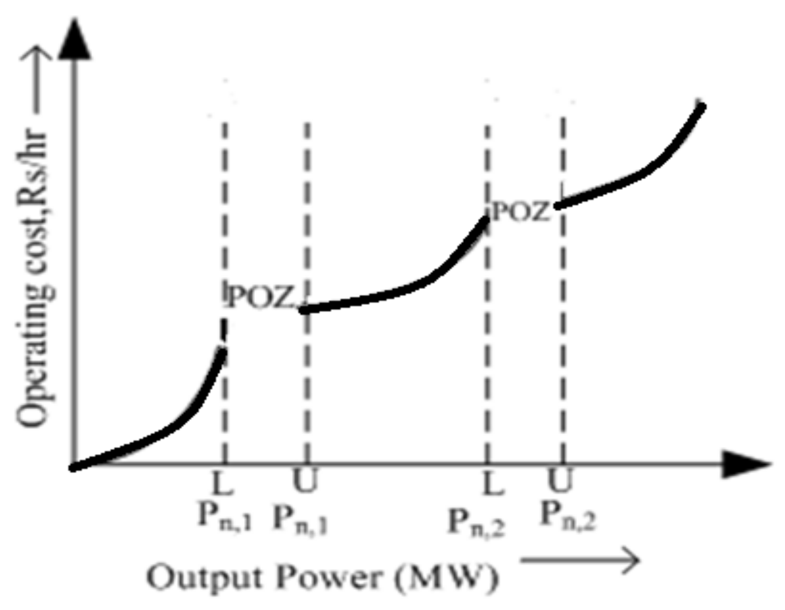
3.1.4. Prohibited Operating Zones
4. Slime Mould Algorithm
4.1. Mathematical Modeling of SMA
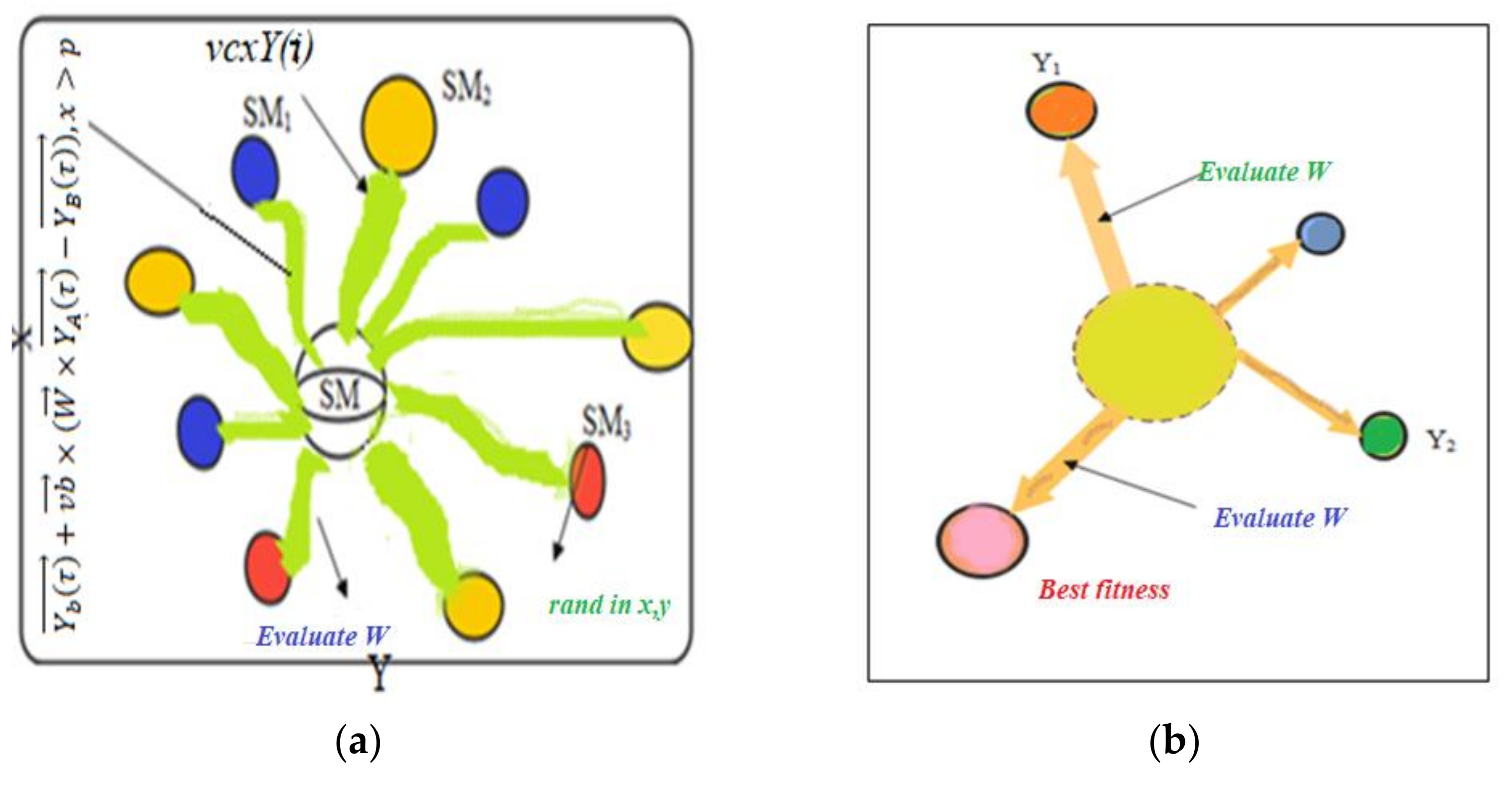
4.1.1. Technique of Approaching Food
4.1.2. Technique of Wrapping Food
4.1.3. Technique of Food Grabble
| Algorithm 1 PSEUDO Code for Slime Mould Algorithm. |
| Initialize the parameter popsize, Max_iteration; Initialize the positions of slime mould (I = 1,2,3,…,n) While Calculate the fitness of all slime mould; update bestfitness, OpF Calculate the W by Equation (17); For each search portion Update,,; Update positions by Equation (19); End For ; End while Return Bestfitness, OpF; |
5. Economic Load Dispatch Flow Chart Using Slime Mould Optimizer
6. Test System Results and Discussion
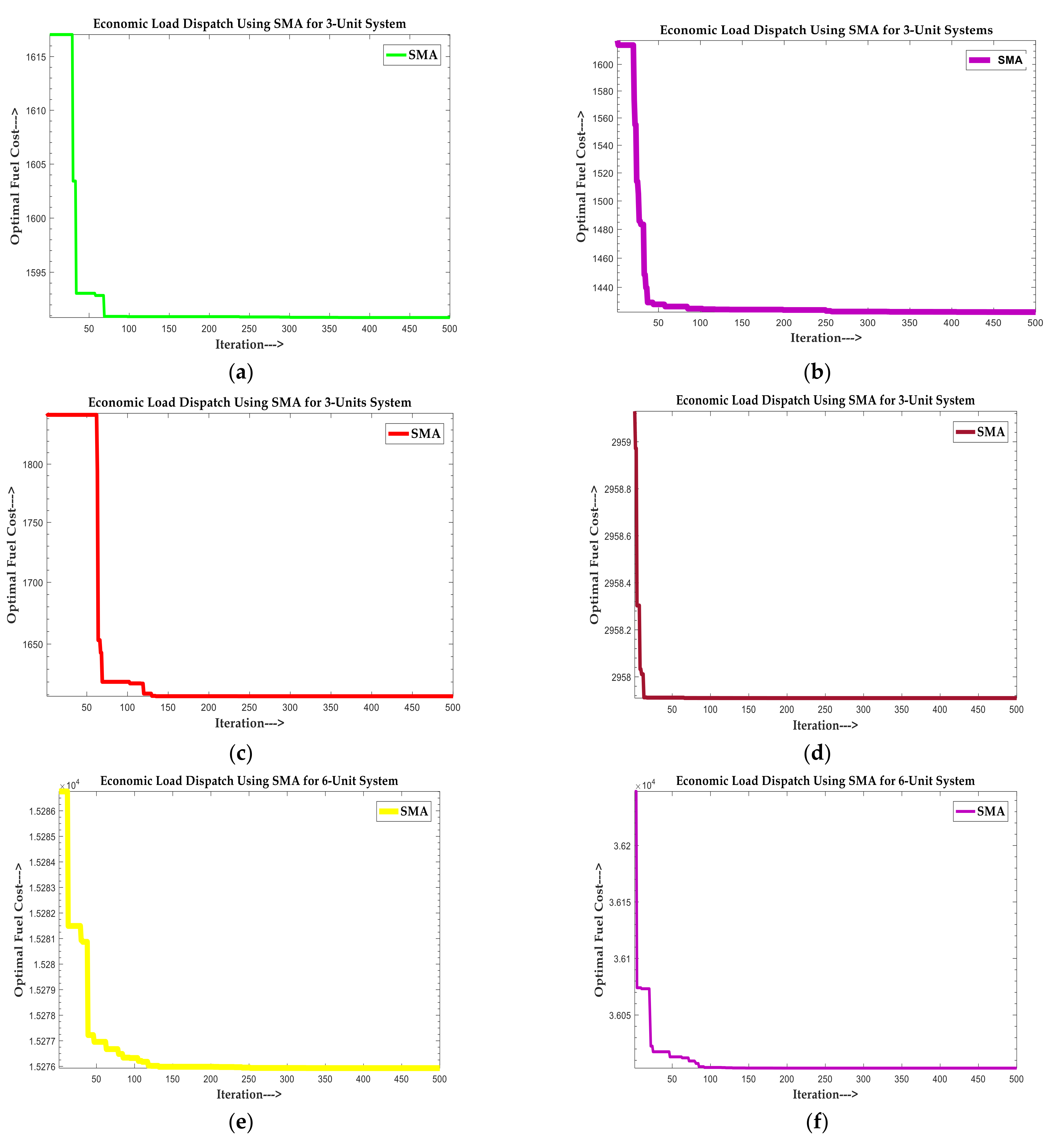
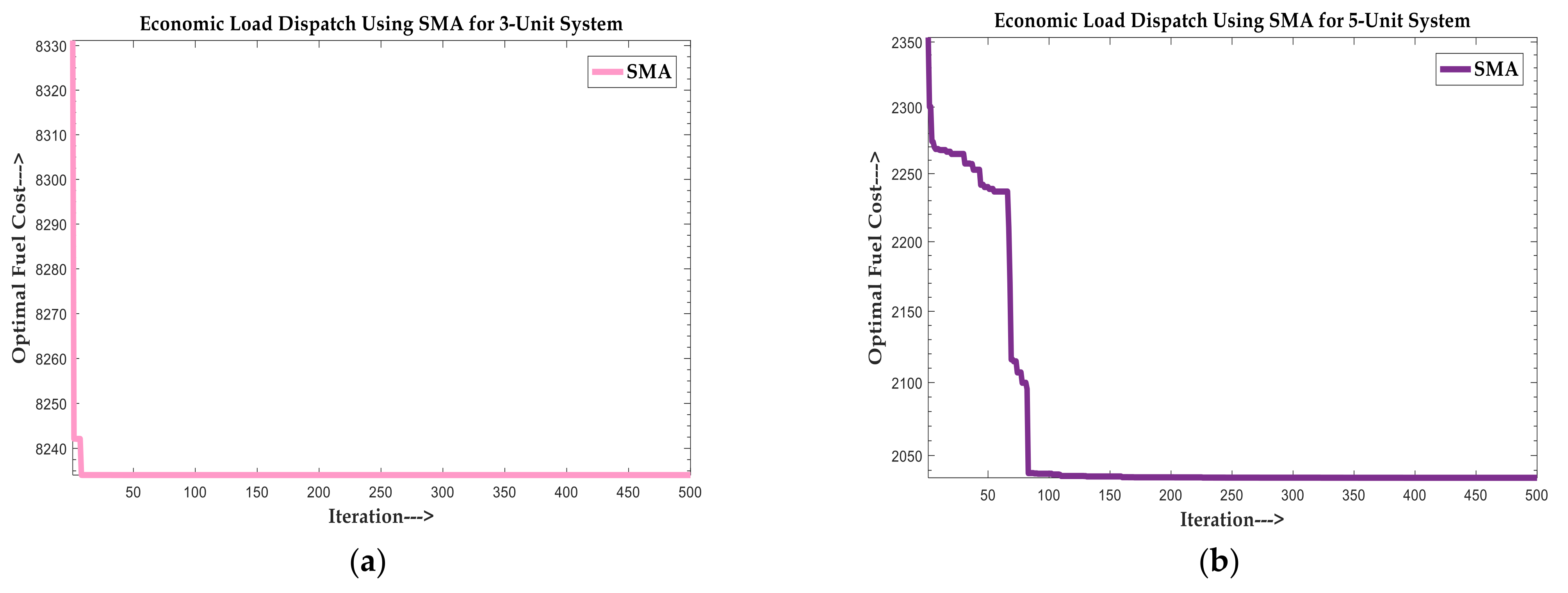
6.1. Test System-I (Small-Scale Power System)
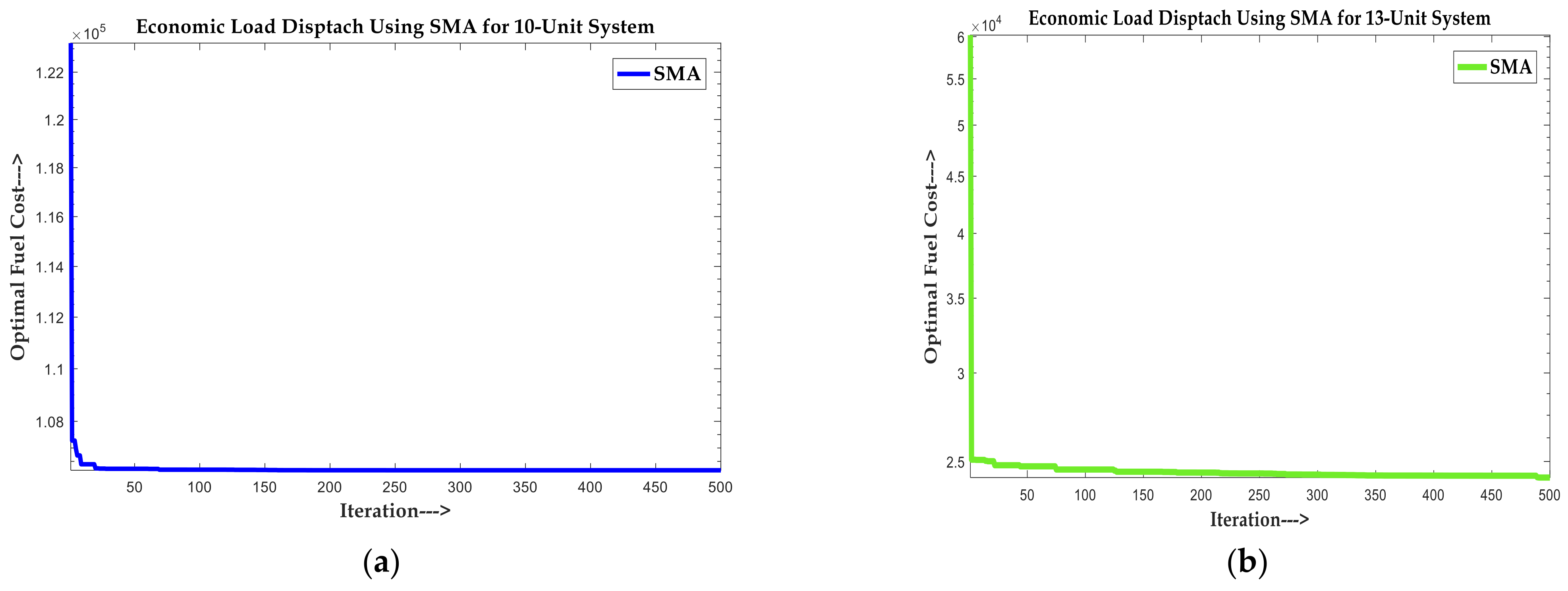
6.2. Test System-II (Medium-Scale Power System)
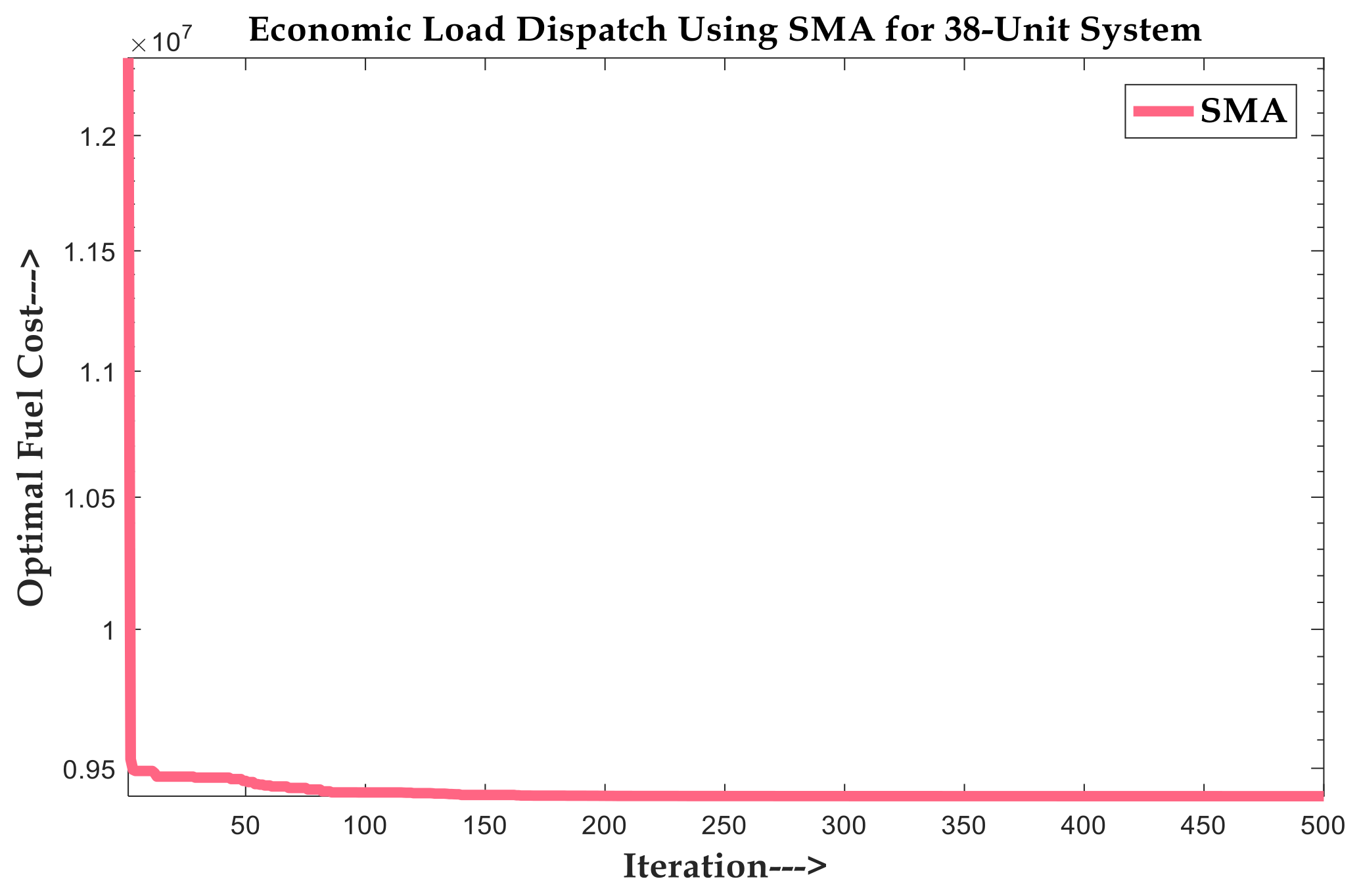
6.3. Test System-III (Large-Scale Power System)
7. Conclusions
Author Contributions
Funding
Institutional Review Board Statement
Informed Consent Statement
Data Availability Statement
Conflicts of Interest
Abbreviations
Appendix A

| Total Units | Pmin (MW) | c ($/h) | b ($/MWh) | a ($/(MW)2h) | Pmax (MW) |
|---|---|---|---|---|---|
| 1 | 10 | 200 | 7.00 | 0.008 | 85 |
| 2 | 10 | 180 | 6.3 | 0.009 | 80 |
| 3 | 10 | 140 | 6.8 | 0.007 | 70 |
| Total Units | Pmin (MW) | c ($/h) | b ($/MWh) | a ($/(MW)2h) | Pmax (MW) |
|---|---|---|---|---|---|
| 1 | 10 | 200 | 7.02 | 0.00816 | 85 |
| 2 | 10 | 180 | 6.35 | 0.00900 | 80 |
| 3 | 10 | 140 | 6.97 | 0.00782 | 70 |
| Total Units | Pmin (MW) | c ($/h) | b ($/MWh) | a ($/(MW)2h) | Pmax (MW) |
|---|---|---|---|---|---|
| 1 | 10 | 200 | 7.02 | 0.00816 | 85 |
| 2 | 10 | 180 | 6.35 | 0.00900 | 80 |
| 3 | 10 | 140 | 6.97 | 0.00782 | 70 |
| Total Units | Pmin (MW) | c ($/h) | b ($/MWh) | a ($/(MW)2h) | Pmax (MW) |
|---|---|---|---|---|---|
| 1 | 50 | 328.13 | 8.663 | 0.00525 | 250 |
| 2 | 5 | 136.91 | 10.04 | 0.00609 | 150 |
| 3 | 15 | 59.16 | 9.76 | 0.00592 | 100 |
| Total Units | Pmin (MW) | c ($/h) | b ($/MWh) | a ($/(MW)2h) | Pmax (MW) |
|---|---|---|---|---|---|
| 1 | 100 | 240 | 7.0 | 0.0070 | 500 |
| 2 | 50 | 200 | 10.0 | 0.0095 | 200 |
| 3 | 80 | 220 | 8.5 | 0.0090 | 300 |
| 4 | 50 | 200 | 11.0 | 0.0090 | 150 |
| 5 | 50 | 220 | 10.5 | 0.0080 | 200 |
| 6 | 50 | 190 | 12.0 | 0.0075 | 120 |
| Total Units | Pmin (MW) | c ($/h) | b ($/MWh) | a ($/(MW)2h) | Pmax (MW) |
|---|---|---|---|---|---|
| 1 | 10 | 756.79886 | 38.53973 | 0.15240 | 125 |
| 2 | 10 | 451.32513 | 46.15916 | 0.10587 | 150 |
| 3 | 35 | 1049.9977 | 40.39655 | 0.02803 | 225 |
| 4 | 35 | 1243.5311 | 38.30553 | 0.03546 | 210 |
| 5 | 130 | 1658.5596 | 36.32782 | 0.02111 | 325 |
| 6 | 125 | 1356.6592 | 38.27041 | 0.01799 | 315 |
| Total Units | Pmin (MW) | e (1/MW) | d ($/h) | c ($/hr) | b ($/MWh) | a ($/(MW)2h) | Pmax (MW) |
|---|---|---|---|---|---|---|---|
| 1 | 100 | 0.0315 | 300 | 561 | 7.92 | 0.001562 | 600 |
| 2 | 100 | 0.042 | 200 | 310 | 7.85 | 0.00194 | 400 |
| 3 | 50 | 0.063 | 150 | 78 | 7.97 | 0.00482 | 200 |
| Total Units | Pmin (MW) | e (1/MW) | d ($/h) | c ($/hr) | b ($/MWh) | a ($/(MW)2h) | Pmax (MW) |
|---|---|---|---|---|---|---|---|
| 1 | 50 | 0.035 | 200.0 | 40.0 | 1.8 | 0.0015 | 300 |
| 2 | 20 | 0.040 | 140.0 | 60.0 | 1.8 | 0.0035 | 125 |
| 3 | 30 | 0.038 | 160.0 | 100.0 | 2.1 | 0.0012 | 175 |
| 4 | 10 | 0.042 | 100.0 | 25.0 | 2.0 | 0.0080 | 75 |
| 5 | 40 | 0.037 | 180.0 | 120.0 | 2.0 | 0.0010 | 250 |
| Total Units | Pmin (MW) | c ($/h) | b ($/MWh) | a ($/(MW)2h) | Pmax (MW) |
|---|---|---|---|---|---|
| 1 | 150 | 671 | 10.1 | 0.000299 | 455 |
| 2 | 150 | 574 | 10.2 | 0.000183 | 455 |
| 3 | 20 | 374 | 8.8 | 0.001126 | 130 |
| 4 | 20 | 374 | 8.8 | 0.001126 | 130 |
| 5 | 150 | 461 | 10.4 | 0.000205 | 470 |
| 6 | 135 | 630 | 10.1 | 0.000301 | 460 |
| 7 | 135 | 548 | 9.8 | 0.000364 | 465 |
| 8 | 60 | 227 | 11.2 | 0.000338 | 300 |
| 9 | 25 | 173 | 11.2 | 0.000807 | 162 |
| 10 | 25 | 175 | 10.7 | 0.001203 | 160 |
| 11 | 20 | 186 | 10.2 | 0.003586 | 80 |
| 12 | 20 | 230 | 9.9 | 0.005513 | 80 |
| 13 | 25 | 225 | 13.1 | 0.000371 | 85 |
| 14 | 15 | 309 | 12.1 | 0.001929 | 55 |
| 15 | 15 | 323 | 12.4 | 0.004447 | 55 |
| Total Units | Pmin (MW) | c ($/h) | b ($/MWh) | a ($/(MW)2h) | Pmax(MW) |
|---|---|---|---|---|---|
| 1 | 150 | 1000 | 18.19 | 0.00068 | 600 |
| 2 | 50 | 970 | 19.26 | 0.00071 | 200 |
| 3 | 50 | 600 | 19.80 | 0.00650 | 200 |
| 4 | 50 | 700 | 19.10 | 0.00500 | 200 |
| 5 | 50 | 420 | 18.10 | 0.00738 | 160 |
| 6 | 20 | 360 | 19.26 | 0.00612 | 100 |
| 7 | 25 | 490 | 17.14 | 0.00790 | 125 |
| 8 | 50 | 660 | 18.92 | 0.00813 | 150 |
| 9 | 50 | 765 | 18.27 | 0.00522 | 200 |
| 10 | 30 | 770 | 18.92 | 0.00573 | 150 |
| 11 | 100 | 800 | 16.69 | 0.00480 | 300 |
| 12 | 150 | 970 | 16.76 | 0.00310 | 500 |
| 13 | 40 | 900 | 17.36 | 0.00850 | 160 |
| 14 | 20 | 700 | 18.70 | 0.00511 | 130 |
| 15 | 25 | 450 | 18.70 | 0.00398 | 185 |
| 16 | 20 | 370 | 14.26 | 0.07120 | 80 |
| 17 | 30 | 480 | 19.14 | 0.00890 | 85 |
| 18 | 30 | 680 | 18.92 | 0.00713 | 120 |
| 19 | 40 | 700 | 18.47 | 0.00622 | 120 |
| 20 | 30 | 850 | 19.79 | 0.00773 | 100 |
| Total Units | Pmin (MW) | e (1/MW) | d ($/h) | c ($/hr) | b ($/MWh) | a ($/(MW)2h) | Pmax (MW) |
|---|---|---|---|---|---|---|---|
| 1 | 10 | 0.0174 | 33 | 1000.403 | 40.5407 | 0.12951 | 55 |
| 2 | 20 | 0.0178 | 25 | 950.606 | 39.5804 | 0.10908 | 80 |
| 3 | 47 | 0.0162 | 32 | 900.705 | 36.5104 | 0.12511 | 120 |
| 4 | 20 | 0.0168 | 30 | 800.705 | 39.5104 | 0.12111 | 130 |
| 5 | 50 | 0.0148 | 30 | 756.799 | 38.539 | 0.15247 | 160 |
| 6 | 70 | 0.0163 | 20 | 451.325 | 46.1592 | 0.10587 | 240 |
| 7 | 60 | 0.0152 | 20 | 1243.531 | 38.3055 | 0.03546 | 300 |
| 8 | 70 | 0.0128 | 30 | 1049.998 | 40.3965 | 0.02803 | 340 |
| 9 | 135 | 0.0136 | 60 | 1658.569 | 36.3278 | 0.02111 | 470 |
| 10 | 150 | 0.0141 | 40 | 1356.659 | 38.2704 | 0.01799 | 470 |
| Total Units | Pmin (MW) | e (1/MW) | d ($/h) | c ($/hr) | b ($/MWh) | a ($/(MW)2h) | Pmax (MW) |
|---|---|---|---|---|---|---|---|
| 1 | 0 | 0.035 | 300 | 550 | 8.10 | 0.00028 | 680 |
| 2 | 0 | 0.042 | 200 | 309 | 8.10 | 0.00056 | 360 |
| 3 | 0 | 0.042 | 200 | 307 | 8.10 | 0.00056 | 360 |
| 4 | 60 | 0.063 | 150 | 240 | 7.74 | 0.00324 | 180 |
| 5 | 60 | 0.063 | 150 | 240 | 7.74 | 0.00324 | 180 |
| 6 | 60 | 0.063 | 150 | 240 | 7.74 | 0.00324 | 180 |
| 7 | 60 | 0.063 | 150 | 240 | 7.74 | 0.00324 | 180 |
| 8 | 60 | 0.063 | 150 | 240 | 7.74 | 0.00324 | 180 |
| 9 | 60 | 0.063 | 150 | 240 | 7.74 | 0.00324 | 180 |
| 10 | 40 | 0.084 | 100 | 126 | 8.6 | 0.00284 | 120 |
| 11 | 40 | 0.084 | 100 | 126 | 8.6 | 0.00284 | 120 |
| 12 | 55 | 0.084 | 100 | 126 | 8.6 | 0.00284 | 120 |
| 13 | 55 | 0.084 | 100 | 126 | 8.6 | 0.00284 | 120 |
| Total Units | Pmin (MW) | c ($/h) | b ($/MWh) | a ($/(MW)2h) | Pmax (MW) |
|---|---|---|---|---|---|
| 1 | 220 | 64,782 | 796.9 | 0.3133 | 550 |
| 2 | 220 | 64,782 | 796.9 | 0.3133 | 550 |
| 3 | 220 | 64,670 | 795.5 | 0.3127 | 550 |
| 4 | 220 | 64,670 | 795.5 | 0.3127 | 550 |
| 5 | 220 | 64,670 | 795.5 | 0.3127 | 550 |
| 6 | 220 | 64,670 | 795.5 | 0.3127 | 550 |
| 7 | 220 | 64,670 | 795.5 | 0.3127 | 550 |
| 8 | 220 | 64,670 | 795.5 | 0.3127 | 550 |
| 9 | 114 | 172,832 | 915.7 | 0.7075 | 500 |
| 10 | 114 | 172,832 | 915.7 | 0.7075 | 500 |
| 11 | 114 | 176,003 | 884.2 | 0.7515 | 500 |
| 12 | 114 | 173,028 | 884.2 | 0.7083 | 500 |
| 13 | 110 | 91,340 | 1250.1 | 0.4211 | 500 |
| 14 | 90 | 63,440 | 1298.6 | 0.5145 | 365 |
| 15 | 82 | 65,468 | 1298.6 | 0.5691 | 365 |
| 16 | 120 | 77,282 | 1290.8 | 0.5691 | 325 |
| 17 | 65 | 190,928 | 238.1 | 2.5881 | 315 |
| 18 | 65 | 285,372 | 1149.5 | 3.8734 | 315 |
| 19 | 65 | 271,676 | 1269.1 | 3.6842 | 315 |
| 20 | 120 | 39,197 | 696.1 | 0.4921 | 272 |
| 21 | 120 | 45,576 | 660.2 | 0.5728 | 272 |
| 22 | 110 | 28,770 | 803.2 | 0.3572 | 260 |
| 23 | 80 | 36,902 | 818.2 | 0.9415 | 190 |
| 24 | 10 | 105,510 | 33.5 | 52.123 | 150 |
| 25 | 60 | 22,233 | 805.4 | 1.1421 | 125 |
| 26 | 55 | 30,953 | 707.1 | 2.0275 | 110 |
| 27 | 35 | 17,044 | 833.6 | 3.0744 | 75 |
| 28 | 20 | 81,079 | 2188.7 | 16.765 | 70 |
| 29 | 20 | 124,767 | 1024.4 | 26.355 | 70 |
| 30 | 20 | 121,915 | 837.1 | 30.575 | 70 |
| 31 | 20 | 120,780 | 1305.2 | 25.098 | 70 |
| 32 | 20 | 104,441 | 716.6 | 33.722 | 60 |
| 33 | 25 | 83,224 | 1633.9 | 23.915 | 60 |
| 34 | 18 | 111,281 | 969.6 | 32.562 | 60 |
| 35 | 8 | 64,142 | 2625.8 | 18.360 | 60 |
| 36 | 25 | 103,519 | 1633.9 | 23.915 | 60 |
| 37 | 20 | 13,547 | 694.7 | 8.482 | 38 |
| 38 | 20 | 13,518 | 655.9 | 9.693 | 38 |
| Total Units | Pmin (MW) | e (1/MW) | d ($/h) | c ($/hr) | b ($/MWh) | a ($/(MW)2h) | Pmax (MW) |
|---|---|---|---|---|---|---|---|
| 1 | 36 | 0.084 | 100 | 94.705 | 6.73 | 0.00690 | 114 |
| 2 | 36 | 0.084 | 100 | 94.705 | 6.73 | 0.00690 | 114 |
| 3 | 60 | 0.084 | 100 | 309.54 | 7.07 | 0.02028 | 120 |
| 4 | 80 | 0.063 | 150 | 369.03 | 8.18 | 0.00942 | 190 |
| 5 | 46 | 0.077 | 120 | 148.89 | 5.35 | 0.01140 | 97 |
| 6 | 68 | 0.084 | 100 | 222.33 | 8.05 | 0.01142 | 140 |
| 7 | 110 | 0.042 | 200 | 287.71 | 8.03 | 0.00357 | 300 |
| 8 | 135 | 0.042 | 200 | 391.98 | 6.99 | 0.00492 | 300 |
| 9 | 135 | 0.042 | 200 | 455.76 | 6.60 | 0.00573 | 300 |
| 10 | 130 | 0.042 | 200 | 722.82 | 12.9 | 0.00606 | 300 |
| 11 | 94 | 0.042 | 200 | 635.20 | 12.9 | 0.00515 | 375 |
| 12 | 94 | 0.042 | 200 | 654.69 | 12.8 | 0.00569 | 375 |
| 13 | 125 | 0.035 | 300 | 913.40 | 12.5 | 0.00421 | 500 |
| 14 | 125 | 0.035 | 300 | 1760.4 | 8.84 | 0.00752 | 500 |
| 15 | 125 | 0.035 | 300 | 1728.3 | 9.15 | 0.00708 | 500 |
| 16 | 125 | 0.035 | 300 | 1728.3 | 9.15 | 0.00708 | 500 |
| 17 | 220 | 0.035 | 300 | 647.85 | 7.97 | 0.00313 | 500 |
| 18 | 220 | 0.035 | 300 | 649.69 | 7.95 | 0.00313 | 500 |
| 19 | 242 | 0.035 | 300 | 647.83 | 7.97 | 0.00313 | 550 |
| 20 | 242 | 0.035 | 300 | 647.81 | 7.97 | 0.00313 | 550 |
| 21 | 254 | 0.035 | 300 | 785.96 | 6.63 | 0.00298 | 550 |
| 22 | 254 | 0.035 | 300 | 785.96 | 6.63 | 0.00298 | 550 |
| 23 | 254 | 0.035 | 300 | 794.53 | 6.66 | 0.00284 | 550 |
| 24 | 254 | 0.035 | 300 | 794.53 | 6.66 | 0.00284 | 550 |
| 25 | 254 | 0.035 | 300 | 801.32 | 7.10 | 0.00277 | 550 |
| 26 | 254 | 0.035 | 300 | 801.32 | 7.10 | 0.00277 | 550 |
| 27 | 10 | 0.077 | 120 | 1055.1 | 3.33 | 0.52124 | 150 |
| 28 | 10 | 0.077 | 120 | 1055.1 | 3.33 | 0.52124 | 150 |
| 29 | 10 | 0.077 | 120 | 1055.1 | 3.33 | 0.52124 | 150 |
| 30 | 47 | 0.077 | 120 | 148.89 | 5.35 | 0.01140 | 97 |
| 31 | 60 | 0.063 | 150 | 222.92 | 6.43 | 0.00160 | 190 |
| 32 | 60 | 0.063 | 150 | 222.92 | 6.43 | 0.00160 | 190 |
| 33 | 60 | 0.063 | 150 | 222.92 | 6.43 | 0.00160 | 190 |
| 34 | 90 | 0.042 | 200 | 107.87 | 8.95 | 0.0001 | 200 |
| 35 | 90 | 0.042 | 200 | 116.58 | 8.62 | 0.0001 | 200 |
| 36 | 90 | 0.042 | 200 | 116.58 | 8.62 | 0.0001 | 200 |
| 37 | 25 | 0.098 | 80 | 307.45 | 5.88 | 0.0161 | 110 |
| 38 | 25 | 0.098 | 80 | 307.45 | 5.88 | 0.0161 | 110 |
| 39 | 25 | 0.098 | 80 | 307.45 | 5.88 | 0.0161 | 110 |
| 40 | 242 | 0.035 | 300 | 647.83 | 7.97 | 0.00313 | 550 |
References
- Panigrahi, C.K.; Chattopadhyay, P.K.; Chakrabarti, R.N.; Basu, M. Simulated Annealing Technique for Dynamic Economic Dispatch. Electr. Power Compon. Syst. 2006, 34, 577–586. [Google Scholar] [CrossRef]
- Jadoun, V.K.; Gupta, N.; Niazi, K.; Swarnkar, A.; Bansal, R. Improved Particle Swarm Optimization for Multi-area Economic Dispatch with Reserve Sharing Scheme. IFAC-PapersOnLine 2015, 48, 161–166. [Google Scholar] [CrossRef]
- Salcedo-Sanz, S. A survey of repair methods used as constraint handling techniques in evolutionary algorithms. Comput. Sci. Rev. 2009, 3, 175–192. [Google Scholar] [CrossRef]
- Cai, J.; Li, Q.; Li, L.; Peng, H.; Yang, Y. A hybrid CPSO–SQP method for economic dispatch considering the valve-point effects. Energy Convers. Manag. 2012, 53, 175–181. [Google Scholar] [CrossRef]
- Zhong, H.; Xia, Q.; Wang, Y.; Kang, C. Dynamic Economic Dispatch Considering Transmission Losses Using Quadratically Constrained Quadratic Program Method. IEEE Trans. Power Syst. 2013, 28, 2232–2241. [Google Scholar] [CrossRef]
- Reid, G.F.; Hasdorff, L. Economic Dispatch Using Quadratic Programming. IEEE Trans. Power Appar. Syst. 1973, PAS-92, 2015–2023. [Google Scholar] [CrossRef]
- Babonneau, F.; Corcos, G.; Drouet, L.; Vial, J.-P. NeatWork: A Tool for the Design of Gravity-Driven Water Distribution Systems for Poor Rural Communities. Interfaces 2019, 49, 129–136. [Google Scholar] [CrossRef] [Green Version]
- Zhan, J.; Wu, Q.H.; Guo, C.; Zhou, X. Fast λ-Iteration Method for Economic Dispatch With Prohibited Operating Zones. IEEE Trans. Power Syst. 2013, 29, 990–991. [Google Scholar] [CrossRef]
- Dibangoye, J.; Doniec, A.; Fakham, H.; Colas, F.; Guillaud, X. Distributed economic dispatch of embedded generation in smart grids. Eng. Appl. Artif. Intell. 2015, 44, 64–78. [Google Scholar] [CrossRef] [Green Version]
- Torreglosa, J.P.; García-Triviño, P.; Fernández-Ramirez, L.M.; Jurado, F. Control based on techno-economic optimization of renewable hybrid energy system for stand-alone applications. Expert Syst. Appl. 2016, 51, 59–75. [Google Scholar] [CrossRef]
- Wang, M.Q.; Han, X.S.; Yang, M. Dynamic economic dispatch with valve point effect, prohibited operation zones, and multiple fuel option. In Proceedings of the IEEE PES Asia-Pacific Power and Energy Engineering Conference (APPEEC), Hong Kong, China, 7–10 December 2014; Volume 29, pp. 1–5. [Google Scholar] [CrossRef]
- Al-Kalaani, Y. Power generation scheduling algorithm using dynamic programming. Nonlinear Anal. Theory Methods Appl. 2009, 71, e641–e650. [Google Scholar] [CrossRef]
- Subathra, M.S.P.; Selvan, S.E.; Victoire, T.A.A.; Christinal, A.H.; Amato, U. A Hybrid With Cross-Entropy Method and Sequential Quadratic Programming to Solve Economic Load Dispatch Problem. IEEE Syst. J. 2015, 9, 1031–1044. [Google Scholar] [CrossRef]
- Li, Z.; Wu, W.; Zhang, B.; Sun, H.; Guo, Q. Dynamic Economic Dispatch Using Lagrangian Relaxation With Multiplier Updates Based on a Quasi-Newton Method. IEEE Trans. Power Syst. 2013, 28, 4516–4527. [Google Scholar] [CrossRef]
- Mohammadi-Ivatloo, B.; Rabiee, A.; Soroudi, A. Nonconvex Dynamic Economic Power Dispatch Problems Solution Using Hybrid Immune-Genetic Algorithm. IEEE Syst. J. 2013, 7, 777–785. [Google Scholar] [CrossRef] [Green Version]
- Gjorgiev, B.; Čepin, M. A multi-objective optimization based solution for the combined economic-environmental power dispatch problem. Eng. Appl. Artif. Intell. 2013, 26, 417–429. [Google Scholar] [CrossRef]
- Singh, N.J.; Dhillon, J.; Kothari, D. Synergic predator-prey optimization for economic thermal power dispatch problem. Appl. Soft Comput. 2016, 43, 298–311. [Google Scholar] [CrossRef]
- Shaw, B.; Mukherjee, V.; Ghoshal, S. Solution of economic dispatch problems by seeker optimization algorithm. Expert Syst. Appl. 2012, 39, 508–519. [Google Scholar] [CrossRef]
- Amjady, N.; Nasiri-Rad, H. Solution of nonconvex and nonsmooth economic dispatch by a new Adaptive Real Coded Genetic Algorithm. Expert Syst. Appl. 2010, 37, 5239–5245. [Google Scholar] [CrossRef]
- Elsayed, S.M.; Sarker, R.; Essam, D.L. A new genetic algorithm for solving optimization problems. Eng. Appl. Artif. Intell. 2014, 27, 57–69. [Google Scholar] [CrossRef]
- Sinha, N.; Chakrabarti, R.; Chattopadhyay, P. Evolutionary programming techniques for economic load dispatch. IEEE Trans. Evol. Comput. 2003, 7, 83–94. [Google Scholar] [CrossRef]
- Yang, X.-S.; Hosseini, S.S.S.; Gandomi, A. Firefly Algorithm for solving non-convex economic dispatch problems with valve loading effect. Appl. Soft Comput. 2012, 12, 1180–1186. [Google Scholar] [CrossRef]
- Neyestani, M.; Farsangi, M.M.; Nezamabadi-Pour, H. A modified particle swarm optimization for economic dispatch with non-smooth cost functions. Eng. Appl. Artif. Intell. 2010, 23, 1121–1126. [Google Scholar] [CrossRef]
- Safari, A.; Shayeghi, H. Iteration particle swarm optimization procedure for economic load dispatch with generator constraints. Expert Syst. Appl. 2011, 38, 6043–6048. [Google Scholar] [CrossRef]
- Wang, L.; Singh, C. Reserve-constrained multiarea environmental/economic dispatch based on particle swarm optimization with local search. Eng. Appl. Artif. Intell. 2009, 22, 298–307. [Google Scholar] [CrossRef]
- Aydın, D.; Özyön, S. Solution to non-convex economic dispatch problem with valve point effects by incremental artificial bee colony with local search. Appl. Soft Comput. 2013, 13, 2456–2466. [Google Scholar] [CrossRef]
- Ghasemi, M.; Taghizadeh, M.; Ghavidel, S.; Abbasian, A. Colonial competitive differential evolution: An experimental study for optimal economic load dispatch. Appl. Soft Comput. 2016, 40, 342–363. [Google Scholar] [CrossRef]
- Farhat, I.; El-Hawary, M. Dynamic adaptive bacterial foraging algorithm for optimum economic dispatch with valve-point effects and wind power. IET Gener. Transm. Distrib. 2010, 4, 989–999. [Google Scholar] [CrossRef]
- Lin, W.-M.; Cheng, F.-S.; Tsay, M.-T. An improved tabu search for economic dispatch with multiple minima. IEEE Trans. Power Syst. 2002, 17, 108–112. [Google Scholar] [CrossRef]
- Pothiya, S.; Ngamroo, I.; Kongprawechnon, W. Ant colony optimisation for economic dispatch problem with non-smooth cost functions. Int. J. Electr. Power Energy Syst. 2010, 32, 478–487. [Google Scholar] [CrossRef]
- Zare, K.; Haque, M.T.; Davoodi, E. Solving non-convex economic dispatch problem with valve point effects using modified group search optimizer method. Electr. Power Syst. Res. 2012, 84, 83–89. [Google Scholar] [CrossRef]
- Jeddi, B.; Vahidinasab, V. A modified harmony search method for environmental/economic load dispatch of real-world power systems. Energy Convers. Manag. 2014, 78, 661–675. [Google Scholar] [CrossRef]
- Bhattacharya, A.; Chattopadhyay, P.K. Solving complex economic load dispatch problems using biogeography-based optimization. Expert Syst. Appl. 2010, 37, 3605–3615. [Google Scholar] [CrossRef]
- Jiang, X.; Zhou, J.; Wang, H.; Zhang, Y. Dynamic environmental economic dispatch using multiobjective differential evolution algorithm with expanded double selection and adaptive random restart. Int. J. Electr. Power Energy Syst. 2013, 49, 399–407. [Google Scholar] [CrossRef]
- Xiong, G.; Shi, D. Orthogonal learning competitive swarm optimizer for economic dispatch problems. Appl. Soft Comput. 2018, 66, 134–148. [Google Scholar] [CrossRef]
- Elhameed, M.; El-Fergany, A. Water cycle algorithm-based economic dispatcher for sequential and simultaneous objectives including practical constraints. Appl. Soft Comput. 2017, 58, 145–154. [Google Scholar] [CrossRef]
- Bhadoria, A.; Kamboj, V.K.; Sharma, M.; Bath, S.K. A Solution to Non-convex/Convex and Dynamic Economic Load Dispatch Problem Using Moth Flame Optimizer. INAE Lett. 2018, 3, 65–86. [Google Scholar] [CrossRef]
- Bulbul, S.M.A.; Pradhan, M.; Roy, P.K.; Pal, T. Opposition-based krill herd algorithm applied to economic load dispatch problem. Ain Shams Eng. J. 2018, 9, 423–440. [Google Scholar] [CrossRef] [Green Version]
- Chen, X.-L.; Wang, P.-H.; Wang, Q.; Dong, Y.-H. A Two-Stage strategy to handle equality constraints in ABC-based power economic dispatch problems. Soft Comput. 2019, 23, 6679–6696. [Google Scholar] [CrossRef]
- Mohammadi, F.; Abdi, H. A modified crow search algorithm (MCSA) for solving economic load dispatch problem. Appl. Soft Comput. 2018, 71, 51–65. [Google Scholar] [CrossRef]
- Rezaie, H.; Kazemi-Rahbar, M.H.; Vahidi, B.; Rastegar, H. Solution of combined economic and emission dispatch problem using a novel chaotic improved harmony search algorithm. J. Comput. Des. Eng. 2019, 6, 447–467. [Google Scholar] [CrossRef]
- Pandey, V.C.; Jadoun, V.K.; Gupta, N.; Niazi, K.R.; Swarnkar, A. Improved Fireworks Algorithm with Chaotic Sequence Operator for Large-Scale Non-convex Economic Load Dispatch Problem. Arab. J. Sci. Eng. 2017, 43, 2919–2929. [Google Scholar] [CrossRef]
- Ghorbani, N.; Babaei, E. Exchange market algorithm for economic load dispatch. Int. J. Electr. Power Energy Syst. 2016, 75, 19–27. [Google Scholar] [CrossRef]
- Chen, G.; Ding, X. Optimal economic dispatch with valve loading effect using self-adaptive firefly algorithm. Appl. Intell. 2014, 42, 276–288. [Google Scholar] [CrossRef]
- Labbi, Y.; Ben Attous, D.; Gabbar, H.A.; Mahdad, B.; Zidan, A. A new rooted tree optimization algorithm for economic dispatch with valve-point effect. Int. J. Electr. Power Energy Syst. 2016, 79, 298–311. [Google Scholar] [CrossRef]
- Modiri-Delshad, M.; Kaboli, S.H.A.; Taslimi-Renani, E.; Rahim, N.A. Backtracking search algorithm for solving economic dispatch problems with valve-point effects and multiple fuel options. Energy 2016, 116, 637–649. [Google Scholar] [CrossRef]
- Kamboj, V.K.; Bhadoria, A.; Bath, S.K. Solution of non-convex economic load dispatch problem for small-scale power systems using ant lion optimizer. Neural Comput. Appl. 2016, 28, 2181–2192. [Google Scholar] [CrossRef]
- Pradhan, M.; Roy, P.; Pal, T. Oppositional based grey wolf optimization algorithm for economic dispatch problem of power system. Ain Shams Eng. J. 2018, 9, 2015–2025. [Google Scholar] [CrossRef]
- Zou, D.; Li, S.; Wang, G.-G.; Li, Z.; Ouyang, H. An improved differential evolution algorithm for the economic load dispatch problems with or without valve-point effects. Appl. Energy 2016, 181, 375–390. [Google Scholar] [CrossRef]
- Fu, C.; Zhang, S.; Chao, K.-H. Energy Management of a Power System for Economic Load Dispatch Using the Artificial Intelligent Algorithm. Electronics 2020, 9, 108. [Google Scholar] [CrossRef] [Green Version]
- Adarsh, B.R.; Raghunathan, T.; Jayabarathi, T.; Yang, X.-S. Economic dispatch using chaotic bat algorithm. Energy 2016, 96, 666–675. [Google Scholar] [CrossRef]
- Elsayed, W.; Hegazy, Y.G.; El-Bages, M.S.; Bendary, F.M. Improved Random Drift Particle Swarm Optimization With Self-Adaptive Mechanism for Solving the Power Economic Dispatch Problem. IEEE Trans. Ind. Inform. 2017, 13, 1017–1026. [Google Scholar] [CrossRef]
- Taheri, B.; Aghajani, G.; Sedaghat, M. Economic dispatch in a power system considering environmental pollution using a multi-objective particle swarm optimization algorithm based on the Pareto criterion and fuzzy logic. Int. J. Energy Environ. Eng. 2017, 8, 99–107. [Google Scholar] [CrossRef] [Green Version]
- Al-Betar, M.A.; Awadallah, M.A. Island bat algorithm for optimization. Expert Syst. Appl. 2018, 107, 126–145. [Google Scholar] [CrossRef]
- Chen, X. Novel dual-population adaptive differential evolution algorithm for large-scale multi-fuel economic dispatch with valve-point effects. Energy 2020, 203, 117874. [Google Scholar] [CrossRef]
- He, X.; Rao, Y.; Huang, J. A novel algorithm for economic load dispatch of power systems. Neurocomputing 2016, 171, 1454–1461. [Google Scholar] [CrossRef]
- Kaboli, S.H.A.; Alqallaf, A.K. Solving non-convex economic load dispatch problem via artificial cooperative search algorithm. Expert Syst. Appl. 2019, 128, 14–27. [Google Scholar] [CrossRef]
- Zhan, J.; Wu, Q.H.; Guo, C.; Zhou, X. Economic Dispatch With Non-Smooth Objectives—Part II: Dimensional Steepest Decline Method. IEEE Trans. Power Syst. 2014, 30, 722–733. [Google Scholar] [CrossRef]
- Basu, M. Hybridization of bee colony optimization and sequential quadratic programming for dynamic economic dispatch. Int. J. Electr. Power Energy Syst. 2013, 44, 591–596. [Google Scholar] [CrossRef]
- Duvvuru, N.; Swarup, S. A Hybrid Interior Point Assisted Differential Evolution Algorithm for Economic Dispatch. IEEE Trans. Power Syst. 2010, 26, 541–549. [Google Scholar] [CrossRef]
- Bhattacharya, A.; Chattopadhyay, P. Hybrid differential evolution with biogeography-based optimization algorithm for solution of economic emission load dispatch problems. Expert Syst. Appl. 2011, 38, 14001–14010. [Google Scholar] [CrossRef]
- Victoire, T.A.A.; Jeyakumar, A. Hybrid PSO–SQP for economic dispatch with valve-point effect. Electr. Power Syst. Res. 2004, 71, 51–59. [Google Scholar] [CrossRef]
- Malik, T.N.; Asar, A.U.; Wyne, M.F.; Akhtar, S. A new hybrid approach for the solution of nonconvex economic dispatch problem with valve-point effects. Electr. Power Syst. Res. 2010, 80, 1128–1136. [Google Scholar] [CrossRef]
- Wang, Y.; Zhou, J.; Lu, Y.; Qin, H.; Wang, Y. Chaotic self-adaptive particle swarm optimization algorithm for dynamic economic dispatch problem with valve-point effects. Expert Syst. Appl. 2011, 38, 14231–14237. [Google Scholar] [CrossRef]
- Yaşar, C.; Özyön, S. A new hybrid approach for nonconvex economic dispatch problem with valve-point effect. Energy 2011, 36, 5838–5845. [Google Scholar] [CrossRef]
- Yang, L.; Fraga, E.S.; Papageorgiou, L.G. Mathematical programming formulations for non-smooth and non-convex electricity dispatch problems. Electr. Power Syst. Res. 2013, 95, 302–308. [Google Scholar] [CrossRef]
- Pan, S.; Jian, J.; Yang, L. A hybrid MILP and IPM approach for dynamic economic dispatch with valve-point effects. Int. J. Electr. Power Energy Syst. 2018, 97, 290–298. [Google Scholar] [CrossRef] [Green Version]
- Alawode, K.; Jubril, A.; Kehinde, L.; Ogunbona, P. Semidefinite programming solution of economic dispatch problem with non-smooth, non-convex cost functions. Electr. Power Syst. Res. 2018, 164, 178–187. [Google Scholar] [CrossRef]
- Ding, T.; Bo, R.; Li, F.; Sun, H. A Bi-Level Branch and Bound Method for Economic Dispatch With Disjoint Prohibited Zones Considering Network Losses. IEEE Trans. Power Syst. 2014, 30, 2841–2855. [Google Scholar] [CrossRef]
- Ding, T.; Bo, R.; Gu, W.; Sun, H. Big-M Based MIQP Method for Economic Dispatch With Disjoint Prohibited Zones. IEEE Trans. Power Syst. 2013, 29, 976–977. [Google Scholar] [CrossRef]
- Jabr, R.A. Solution to Economic Dispatching With Disjoint Feasible Regions Via Semidefinite Programming. IEEE Trans. Power Syst. 2011, 27, 572–573. [Google Scholar] [CrossRef]
- Boqiang, R.; Chuanwen, J. A review on the economic dispatch and risk management considering wind power in the power market. Renew. Sustain. Energy Rev. 2009, 13, 2169–2174. [Google Scholar] [CrossRef]
- Peng, M.; Liu, L.; Jiang, C. A review on the economic dispatch and risk management of the large-scale plug-in electric vehicles (PHEVs)-penetrated power systems. Renew. Sustain. Energy Rev. 2012, 16, 1508–1515. [Google Scholar] [CrossRef]
- Mahdi, F.P.; Vasant, P.; Kallimani, V.; Watada, J.; Fai, P.Y.S.; Abdullah-Al-Wadud, M. A holistic review on optimization strategies for combined economic emission dispatch problem. Renew. Sustain. Energy Rev. 2018, 81, 3006–3020. [Google Scholar] [CrossRef]
- Liaquat, S.; Zia, M.; Benbouzid, M. Modeling and Formulation of Optimization Problems for Optimal Scheduling of Multi-Generation and Hybrid Energy Systems: Review and Recommendations. Electronics 2021, 10, 1688. [Google Scholar] [CrossRef]
- Panigrahi, T.K.; Sahoo, A.K.; Behera, A. A review on application of various heuristic techniques to combined economic and emission dispatch in a modern power system scenario. Energy Procedia 2017, 138, 458–463. [Google Scholar] [CrossRef]
- Qu, B.-Y.; Zhu, Y.; Jiao, Y.; Wu, M.; Suganthan, P.N.; Liang, J. A survey on multi-objective evolutionary algorithms for the solution of the environmental/economic dispatch problems. Swarm Evol. Comput. 2018, 38, 1–11. [Google Scholar] [CrossRef]
- Liaquat, S.; Fakhar, M.S.; Kashif, S.A.R.; Rasool, A.; Saleem, O.; Zia, M.F.; Padmanaban, S. Application of Dynamically Search Space Squeezed Modified Firefly Algorithm to a Novel Short Term Economic Dispatch of Multi-Generation Systems. IEEE Access 2020, 9, 1918–1939. [Google Scholar] [CrossRef]
- Nazari-Heris, M.; Jabari, F.; Mohammadi-Ivatloo, B.; Asadi, S.; Habibnezhad, M. An updated review on multi-carrier energy systems with electricity, gas, and water energy sources. J. Clean. Prod. 2020, 275, 123136. [Google Scholar] [CrossRef]
- Camp, W.G. A Method of Cultivating Myxomycete Plasmodia. Bull. Torrey Bot. Club. 2016, 63, 205–210. [Google Scholar] [CrossRef]
- Seifriz, W. Protoplasmic streaming. Bot. Rev. 1943, 9, 49–123. [Google Scholar] [CrossRef]
- Nakagaki, T.; Yamada, H.; Ueda, T. Interaction between cell shape and contraction pattern in the Physarum plasmodium. Biophys. Chem. 2000, 84, 195–204. [Google Scholar] [CrossRef]
- Howard, F.L. The Life History of Physarumpolycephalum. Am. J. Bot. 1931, 18, 116–133. [Google Scholar] [CrossRef]
- Latty, T.; Beekman, M. Speed–accuracy trade-offs during foraging decisions in the acellular slime mouldPhysarumpolycephalum. Proc. R. Soc. B Boil. Sci. 2011, 278, 539–545. [Google Scholar] [CrossRef] [PubMed] [Green Version]
- Latty, T.; Beekman, M. Slime moulds use heuristics based on within-patch experience to decide when to leave. J. Exp. Biol. 2015, 218, 1175–1179. [Google Scholar] [CrossRef] [Green Version]
- Li, S.; Chen, H.; Wang, M.; Heidari, A.A.; Mirjalili, S. Slime mould algorithm: A new method for stochastic optimization. Future Gener. Comput. Syst. 2020, 111, 300–323. [Google Scholar] [CrossRef]
- Sharma, U.; Moses, B. Analysis and optimization of economic load dispatch using soft computing techniques. In Proceedings of the 2016 International Conference on Electrical, Electronics, and Optimization Techniques (ICEEOT), Chennai, India, 3–5 March 2016; pp. 4035–4040. [Google Scholar] [CrossRef]
- Kamboj, V.K.; Bath, S.K.; Dhillon, J.S. Solution of non-convex economic load dispatch problem using Grey Wolf Optimizer. Neural Comput. Appl. 2016, 27, 1301–1316. [Google Scholar] [CrossRef]
- Zaraki, A.; Bin Othman, M.F. Implementing Particle Swarm Optimization to Solve Economic Load Dispatch Problem. In Proceedings of the 2009 International Conference of Soft Computing and Pattern Recognition, Malacca, Malaysia, 4–7 December 2009; pp. 60–65. [Google Scholar] [CrossRef]
- Saxena, N.; Ganguli, S. Solar and Wind Power Estimation and Economic Load Dispatch Using Firefly Algorithm. Procedia Comput. Sci. 2015, 70, 688–700. [Google Scholar] [CrossRef] [Green Version]
- Hardiansyah, H.; Junaidi, J.; Ms, Y. Solving Economic Load Dispatch Problem Using Particle Swarm Optimization Technique. Int. J. Intell. Syst. Appl. 2012, 4, 12–18. [Google Scholar] [CrossRef]
- Subramanian, R.; Thanushkodi, K.; Prakash, A. An efficient meta heuristic algorithm to solve economic load dispatch problems. Iran. J. Electr. Electron. Eng. 2013, 9, 246–252. [Google Scholar]
- Zhang, J.; Wang, Y.; Wang, R.; Hou, G. A New Particle Swarm Optimization Solution to Nonconvex Economic Dispatch Problem. Comput. Vis. 2010, 6145, 191–197. [Google Scholar] [CrossRef]
- Storn, R.; Price, K. Differential evolution—A simple and efficient heuristic for global optimization over continuous spaces. J. Glob. Optim. 1997, 11, 341–359. [Google Scholar] [CrossRef]
- Gaing, Z.-L. Particle swarm optimization to solving the economic dispatch considering the generator constraints. IEEE Trans. Power Syst. 2003, 18, 1187–1195. [Google Scholar] [CrossRef]
- Alam, F.; Thayananthan, V.; Katib, I. Analysis of round-robin load-balancing algorithm with adaptive and predictive approaches. In Proceedings of the 2016 UKACC 11th International Conference on Control (CONTROL), Belfast, UK, 31 August–2 September 2016; Institute of Electrical and Electronics Engineers (IEEE): Piscataway, NJ, USA, 2016; pp. 1–7. [Google Scholar]
- Kuo, C.-C. A Novel Coding Scheme for Practical Economic Dispatch by Modified Particle Swarm Approach. IEEE Trans. Power Syst. 2008, 23, 1825–1835. [Google Scholar] [CrossRef]
- Bhattacharya, A.; Chattopadhyay, P.K. Biogeography-Based Optimization for Different Economic Load Dispatch Problems. IEEE Trans. Power Syst. 2009, 25, 1064–1077. [Google Scholar] [CrossRef]
- Nayak, S.K.; Krishnanand, K.; Panigrahi, B.; Rout, P. Application of Artificial Bee Colony to economic load dispatch problem with ramp rate limits and prohibited operating zones. In Proceedings of the 2009 World Congress on Nature & Biologically Inspired Computing (NaBIC), Coimbatore, India, 9–11 December 2009; pp. 1237–1242. [Google Scholar] [CrossRef]
- Chaturvedi, K.T.; Pandit, M.; Srivastava, L. Self-Organizing Hierarchical Particle Swarm Optimization for Nonconvex Economic Dispatch. IEEE Trans. Power Syst. 2008, 23, 1079–1087. [Google Scholar] [CrossRef]
- Bestha, M.; Reddy, K.H.; Hemakeshavulu, O. Economic Load Dispatch Downside with Valve—Point Result Employing a Binary Bat Formula. Int. J. Electr. Comput. Eng. (IJECE) 2014, 4, 101–107. [Google Scholar] [CrossRef]
- Coelho, L.D.S.; Lee, C.-S. Solving economic load dispatch problems in power systems using chaotic and Gaussian particle swarm optimization approaches. Int. J. Electr. Power Energy Syst. 2008, 30, 297–307. [Google Scholar] [CrossRef]
- Hemamalini, S.; Simon, S.P. Artificial Bee Colony Algorithm for Economic Load Dispatch Problem with Non-smooth Cost Functions. Electr. Power Compon. Syst. 2010, 38, 786–803. [Google Scholar] [CrossRef]
- Su, C.-T.; Lin, C.-T. New approach with a Hopfield modeling framework to economic dispatch. IEEE Trans. Power Syst. 2000, 15, 541–545. [Google Scholar] [CrossRef]
- Spea, S.R. Solving practical economic load dispatch problem using crow search algorithm. Int. J. Electr. Comput. Eng. (IJECE) 2020, 10, 3431–3440. [Google Scholar] [CrossRef]
- Rizk-Allah, R.M.; Mageed, H.M.A.; El-Sehiemy, R.; Aleem, S.A.; El Shahat, A. A New Sine Cosine Optimization Algorithm for Solving Combined Non-Convex Economic and Emission Power Dispatch Problems. Int. J. Energy Convers. (IRECON) 2017, 5, 180. [Google Scholar] [CrossRef]
- Bhullar, P.S.; Dhami, J.K. PSO-TVAC-Based Economic Load Dispatch with Valve-Point Loading. In Proceedings of the Fifth International Conference on Soft Computing for Problem Solving; Springer: Singapore, 2016; Volume 436, pp. 823–832. [Google Scholar] [CrossRef]
- Xu, J.; Yan, F.; Yun, K.; Su, L.; Li, F.; Guan, J. Noninferior Solution Grey Wolf Optimizer with an Independent Local Search Mechanism for Solving Economic Load Dispatch Problems. Energies 2019, 12, 2274. [Google Scholar] [CrossRef] [Green Version]
- Chaturvedi, K.T.; Pandit, M.; Srivastava, L. Particle swarm optimization with time varying acceleration coefficients for non-convex economic power dispatch. Int. J. Electr. Power Energy Syst. 2009, 31, 249–257. [Google Scholar] [CrossRef]


| Transfer of Power Generating Units | ||||||
|---|---|---|---|---|---|---|
| Method | Fuel Price (Rs./h) | Required Power in Demand (MW) | G1 | G2 | G3 | Loss in Power, PLoss (MW) |
| Grey Wolf Optimizer [88] | 1597.4815 | 150 | 30.4998 | 64.6208 | 54.8994 | 2.3444 |
| Quadratic Programming [89] | 1596 | 150 | 32.8116 | 64.5973 | 54.9329 | 2.3419 |
| Lambda Method [87] | 1599.98 | 150 | 33.4701 | 64.0974 | 55.1011 | 2.6686 |
| Particle Swarm Optimization [87] | 1597.48 | 150 | 32.8101 | 64.595 | 54.9369 | 2.342 |
| Genetic Algorithm [87] | 1600 | 150 | 34.4895 | 64.0299 | 54.1534 | 2.6728 |
| Slime Mould Algorithm | 1590.627083 | 150 | 10 | 76.42812 | 64.24508 | 0.336600019 |
| Transfer of Power Generating Units | ||||||
|---|---|---|---|---|---|---|
| Method | Fuel Price (Rs./h) | Required Power in Demand (MW) | G1 | G2 | G3 | Loss in Power, PLoss (MW) |
| Lambda Algorithm [90] | 1422.159458 | 125 | - | - | - | 2.084005739 |
| Firefly Algorithm [90] | 1421.561972 | 125 | - | - | - | 1.964774407 |
| Slime Mould Algorithm | 1413.990605 | 125 | 10 | 70.21971 | 45.41896 | 0.319332527 |
| Transfer of Power Generating Units | ||||||
|---|---|---|---|---|---|---|
| Method | Fuel Price (Rs./hr) | Required Power in Demand (MW) | G1 | G2 | G3 | Loss in Power, PLoss (MW) |
| Lambda Algorithm [90] | 1625.4586 | 150 | - | - | - | 2.813864755 |
| Firefly Algorithm [90] | 1616.921725 | 150 | 32.729 | 63.843 | 56.151 | 2.721760653 |
| Slime Mould Algorithm | 1608.866334 | 150 | 10 | 80 | 60.74528 | 0.372641 |
| Transfer of Power Generating Units | ||||||
|---|---|---|---|---|---|---|
| Method | Fuel Price (Rs./h) | Required Power in Demand (MW) | G1 | G2 | G3 | Loss in Power, PLoss (MW) |
| Particle Swarm Optimization [91] | 2959.98 | 250 | 151.09 | 42.04 | 56.87 | 0 |
| Slime Mould Algorithm | 2957.909554 | 250 | 165.7781 | 29.85793 | 54.36396 | 0 |
| Transfer of Power Generating Units | |||||||||
|---|---|---|---|---|---|---|---|---|---|
| Method | Fuel Price (Rs./h) | Required Power in Demand (MW) | G1 | G2 | G3 | G4 | G5 | G6 | Loss in Power, PLoss (MW) |
| New Particle Swarm Optimization-local random search [93] | 15,450 | 1263 | 446.96 | 173.3944 | 262.3436 | 139.5120 | 164.7089 | 89.0162 | 12.9361 |
| Differential Evaluation [94] | 15,445.90 | 1263 | 400.00 | 186.55 | 289.00 | 150.00 | 200.00 | 50.00 | 12.52 |
| New Particle Swarm Optimization [93] | 15,450 | 1263 | 447.4734 | 173.1012 | 262.6804 | 139.4156 | 165.3002 | 87.9761 | 12.9470 |
| Simulated Annealing Algorithm [92] | 15,466.00 | 1263 | 447.08 | 173.18 | 263.92 | 139.06 | 165.58 | 86.63 | 12.47 |
| Classical Particle Swarm Optimization 2(CPSO2) [24] | 15,446 | 1263 | 434.4295 | 173.3231 | 274.4735 | 128.0598 | 179.4759 | 85.9281 | 12.9582 |
| Particle Swarm Optimization [95] | 15,450 | 1263 | 447.50 | 173.32 | 263.47 | 139.06 | 165.48 | 87.13 | 12.958 |
| Genetic Algorithm [96] | 15,459 | 1263 | 474.81 | 178.64 | 262.21 | 134.28 | 151.90 | 74.18 | 13.022 |
| New Modified Particle Swarm Optimization [97] | 15,447 | 1263 | 446.71 | 173.01 | 265.00 | 139.00 | 165.23 | 86.78 | 12.733 |
| Particle Swarm Optimization –local random search [93] | 15,450 | 1263 | 47.4440 | 173.3430 | 263.3646 | 139.1279 | 165.5076 | 87.1698 | 12.9571 |
| Firefly Algorithm [92] | 15,443 | 1263 | 445.08 | 173.08 | 264.42 | 139.59 | 166.02 | 87.21 | 12.4 |
| Classical Particle Swarm Optimization 1(CPSO1) [24] | 15,447 | 1263 | 434.4236 | 173.4385 | 274.2247 | 128.0183 | 179.7042 | 85.9082 | 12.9583 |
| Biogeography-Based Optimization [98] | 15,443.0963 | 1263 | 447.3997 | 173.2392 | 263.3163 | 138.0006 | 165.4104 | 87.07979 | 12.464 |
| Iteration Particle Swarm Optimization (IPSO) [24] | 15,444 | 1263 | 440.5711 | 179.8365 | 261.3798 | 131.9134 | 170.9823 | 90.8241 | 12.548 |
| Artificial Bee Colony Optimization [99] | 15,445.90 | 1263 | 438.65 | 167.90 | 262.82 | 136.77 | 171.76 | 97.67 | 12.52 |
| Self-Organizing Hierarchical Particle Swarm Optimization [100] | 15,446.02 | 1263 | 438.21 | 172.58 | 257.42 | 141.09 | 179.37 | 86.88 | 12.55 |
| Slime Mould Algorithm | 15,275.9304 | 1263 | 446.6889 | 171.254 | 264.1159 | 125.2018495 | 172.1444773 | 83.59471703 | 0 |
| Transfer of Power Generating Units | |||||||||
|---|---|---|---|---|---|---|---|---|---|
| Method | Fuel Price (Rs./h) | Required Power in Demand (MW) | G1 | G2 | G3 | G4 | G5 | G6 | Loss in Power, PLoss (MW) |
| Conventional Method [91] | 36,914.01 | 700 | 28.33 | 10 | 118.95 | 118.67 | 230.75 | 212.80 | 19.50 |
| Particle Swarm Optimization [91] | 36,912.16 | 700 | 28.28 | 10 | 119.02 | 118.79 | 230.78 | 212.56 | 19.43 |
| Slime Mould Algorithm | 36,003.12394 | 700 | 24.9763 | 10 | 102.6661 | 110.6311 238 | 232.677 8302 | 219.0486 296 | 0 |
| Transfer of Power Generating Units | ||||||
|---|---|---|---|---|---|---|
| Method | Fuel Price (Rs./h) | Required Power in Demand (MW) | G1 | G2 | G3 | Loss in Power, PLoss(MW) |
| CPSO [4] | 8234.07 | 850 | 300.267 | 400 | 149.733 | NR |
| GA [101] | 8575.64 | 850 | 382.2552 | 340.3202 | 127.4184 | NR |
| EP-SQP [4] | 8234.07 | 850 | 300.264 | 400 | 149.733 | NR |
| DE [49] | 8234.07173 | 850 | 300.2668999 | 400 | 149.7331001 | NR |
| PSO [4] | 8234.07 | 850 | 300.267 | 400 | 149.733 | NR |
| ABC [101] | 8253.10 | 850 | 300.266 | 400 | 149.733 | NR |
| PSO-SQP [4] | 8234.07 | 850 | 300.268 | 400 | 149.733 | NR |
| EP [4] | 8234.07 | 850 | 300.264 | 400 | 149.736 | NR |
| Lambda [101] | 8575.68 | 850 | 382.258 | 340.323 | 127.419 | NR |
| CPSO–SQP [4] | 8234.07 | 850 | 300.266 | 400 | 149.734 | NR |
| Slime Mould Algorithm | 8234.07173 | 850 | 300.2668998 | 400 | 149.7331002 | 0 |
| Transfer of Power Generating Units | ||||||||
|---|---|---|---|---|---|---|---|---|
| Method | Fuel Price (Rs./h) | Required Power in Demand (MW) | G1 | G2 | G3 | G4 | G5 | Loss in Power, PLoss (MW) |
| Genetic Algorithm [101] | 2412.538 | 730 | 218.0184 | 109.0092 | 147.5229 | 28.37844 | 227.0275 | NR |
| Particle Swarm Optimization [101] | 2252.572 | 730 | 229.5195 | 125 | 175 | 75 | 125.4804 | NR |
| Lambda [101] | 2412.709 | 730 | 218.028 | 109.014 | 147.535 | 28.380 | 272.042 | NR |
| APSO [101] | 2140.97 | 730 | 225.3845 | 113.020 | 109.4146 | 73.11176 | 209.0692 | NR |
| Slime Mould Algorithm | 2034.972427 | 730 | 229.5195832 | 102.9830227 | 112.6813882 | 74.9999977 | 209.816008 | 0 |
| Method | CPSO1 [24] | ETQ [102] | PSO [102] | ESO [102] | SOH_PSO [24] | PSO(4) [102] | CPSO2 [24] | IPSO [24] | ABC [103] | ES [102] | Hybrid GAPSO [24] | GA [102] | Slime Mould Algorithm |
|---|---|---|---|---|---|---|---|---|---|---|---|---|---|
| Fuel price (Rs. /h) | 32,835 | 32,507.5 | 32,858 | 32,506.6 | 32,751.39 | 32,508.12 | 32,834 | 32,709 | 32,707.85 | 32,568.54 | 32,724 | 33,113 | 32,259.69325 |
| Required Power in Demand (MW) | 2630 | 2630 | 2630 | 2630 | 2630 | 2630 | 2630 | 2630 | 2630 | 2630 | 2630 | 2630 | 2630 |
| G1 | 450.05 | 450 | 439.12 | 456 | 455 | 440.499 | 450.02 | 455 | 455 | 455 | 436.8482 | 415.31 | 455 |
| G2 | 454.04 | 450 | 407.97 | 456 | 380 | 179.5947 | 454.06 | 380 | 380 | 380 | 409.6974 | 359.72 | 454.7336 |
| G3 | 124.82 | 130 | 119.63 | 130 | 130 | 21.0524 | 124.81 | 129.97 | 130 | 130 | 117.0074 | 104.42 | 130 |
| G4 | 124.82 | 130 | 129.99 | 130 | 130 | 87.1376 | 124.81 | 130 | 130 | 150 | 128.2705 | 74.98 | 129.9999991 |
| G5 | 151.03 | 335 | 151.07 | 304.24 | 170 | 360.7675 | 151.06 | 169.93 | 169.9997 | 168.92 | 153.3361 | 380.28 | 288.3104957 |
| G6 | 460 | 455 | 459.99 | 460 | 459.96 | 395.833 | 460 | 459.88 | 460 | 459.34 | 457.4078 | 426.79 | 459.9767033 |
| G7 | 434.53 | 465 | 425.56 | 465 | 430 | 432.0085 | 434.57 | 429.25 | 430 | 430 | 424.4400 | 341.32 | 465 |
| G8 | 148.41 | 60 | 98.56 | 60 | 117.53 | 168.9198 | 148.46 | 60.43 | 71.9698 | 97.42 | 101.1949 | 124.79 | 60.19352401 |
| G9 | 63.61 | 25 | 113.49 | 25 | 77.90 | 162 | 63.59 | 74.78 | 59.1798 | 30.61 | 116.1186 | 133.14 | 25 |
| G10 | 101.13 | 20 | 101.11 | 20 | 119.54 | 138.4343 | 101.12 | 158.02 | 159.8004 | 142.56 | 102.2243 | 89.26 | 25.24209 |
| G11 | 28.656 | 20 | 33.91 | 29.15 | 54.50 | 52.6294 | 28.655 | 80 | 80 | 80 | 35.0317 | 60.06 | 20.04263 |
| G12 | 20.912 | 55 | 79.96 | 59.24 | 80 | 66.8875 | 20.914 | 78.57 | 80 | 85 | 78.8482 | 50 | 61.37133 |
| G13 | 25.001 | 25 | 25. | 25 | 25 | 62.7471 | 25.002 | 25 | 25.0024 | 15 | 27.1292 | 38.77 | 25.00313 |
| G14 | 54.418 | 15 | 41.41 | 17.28 | 17.86 | 47.5574 | 54.414 | 15 | 15.0056 | 15 | 37.1594 | 41.94 | 15.09977 |
| G15 | 20.625 | 15 | 35.61 | 15 | 15 | 27.6065 | 20.624 | 15 | 15.0014 | 15 | 37.0390 | 22.64 | 15.04694 |
| Loss in Power, PLoss (MW) | 32.1302 | 15.8 | 32.42 | 13.79 | 32.28 | 13.6745 | 32.1303 | 30.858 | 13 | 23.85 | 31.75 | 38.28 | 0.010082332 |
| Method | Hopfield Neural Network [104] | Lambda-Iteration Method [102] | Slime Mould Algorithm |
|---|---|---|---|
| Fuel Price (Rs./h) | 62,456.6341 | 62,456.6391 | 60,152.72915 |
| Required Power in Demand (MW) | 2500 | 2500 | 2500 |
| G1 | 512.7804 | 512.7805 | 599.9962 |
| G2 | 169.1035 | 169.1033 | 127.2091 |
| G3 | 126.8897 | 126.8898 | 50.01089 |
| G4 | 102.8656 | 102.8657 | 50 |
| G5 | 113.6836 | 113.6836 | 92.80191 |
| G6 | 73.5709 | 73.5710 | 20.00047 |
| G7 | 115.2876 | 115.2878 | 124.9982 |
| G8 | 116.3994 | 116.3994 | 50 |
| G9 | 100.4063 | 100.4062 | 112.1931 |
| G10 | 106.0267 | 106.0267 | 43.44606 |
| G11 | 150.2395 | 150.2394 | 289.1196 |
| G12 | 292.7647 | 292.7648 | 433.1905 |
| G13 | 119.1155 | 119.1154 | 122.9385 |
| G14 | 30.8342 | 30.8340 | 72.39983 |
| G15 | 115.8056 | 115.8057 | 95.40311 |
| G16 | 36.2545 | 36.2545 | 36.15509 |
| G17 | 66.8590 | 66.8590 | 30.01615 |
| G18 | 87.9720 | 87.9720 | 39.79051 |
| G19 | 100.8033 | 100.8033 | 80.33078 |
| G20 | 54.3050 | 54.3050 | 30 |
| Loss in Power, PLoss(MW) | 91.9669 | 91.9670 | 0 |
| Method | PDE [106] | FPA [106] | MODE [106] | PSO [105] | NSGAII [106] | GSA [106] | PSO-TVAC [107] | ABC_PSO [106] | EMOCA [106] | MSCO [106] | SPEA-2 [106] | Slime Mould Algorithm |
|---|---|---|---|---|---|---|---|---|---|---|---|---|
| Fuel Price (Rs./h) | 113,510 | 113,370 | 113,484 | 107,620 | 113,539 | 113,490 | 107,620 | 113,420 | 113,445 | 110,870 | 113,520 | 106,170.418 |
| Power in Demand (MW) | 2000 | 2000 | 2000 | 2000 | 2000 | 2000 | 2000 | 2000 | 2000 | 2000 | 2000 | 2000 |
| G1 | 54.9853 | 53.188 | 54.9487 | 53.1000 | 51.9515 | 54.9992 | 53.8 | 55 | 55 | 52.8995 | 52.9761 | 54.99996 |
| G2 | 79.3803 | 79.975 | 74.5821 | 79.2000 | 67.2584 | 79.9586 | 78.9 | 80 | 80 | 74.9428 | 72.813 | 79.9999 |
| G3 | 83.9842 | 78.105 | 79.4294 | 112 | 73.6879 | 79.4341 | 109 | 81.14 | 83.5594 | 97.4068 | 78.1128 | 89.30891 |
| G4 | 86.5942 | 97.119 | 80.6875 | 121 | 91.3554 | 85.0000 | 125 | 84.216 | 84.6031 | 95.9554 | 83.6088 | 79.87863 |
| G5 | 144.4386 | 152.74 | 136.8551 | 98.8000 | 134.0522 | 142.1063 | 98.8 | 138.3377 | 146.5632 | 131.8702 | 137.2432 | 66.48786 |
| G6 | 165.7756 | 163.08 | 172.6393 | 100 | 174.9504 | 166.5670 | 90.4 | 167.5086 | 169.2481 | 200.5119 | 172.9188 | 70.00002 |
| G7 | 283.2122 | 258.61 | 283.8233 | 299 | 289.4350 | 292.8749 | 298 | 296.8338 | 300 | 227.9224 | 287.2033 | 290.7383 |
| G8 | 312.7709 | 302.22 | 316.3407 | 320 | 314.0556 | 313.2387 | 330 | 311.5824 | 317.3496 | 303.6511 | 326.4023 | 328.5865 |
| G9 | 440.1135 | 433.21 | 448.5923 | 467 | 455.6978 | 441.1775 | 468 | 420.3363 | 412.9183 | 366.3189 | 448.8814 | 470 |
| G10 | 432.6783 | 466.07 | 436.4287 | 356 | 431.8054 | 428.6306 | 351 | 449.1598 | 434.3133 | 470.0000 | 423.9025 | 470 |
| Loss in Power, PLoss (MW) | 83.9 | 84.3 | 84.33 | NR | 84.25 | 83.9869 | NR | 84.1736 | 83.56 | 21.4789 | 84.1 | 0 |
| Method | GWO [108] | JAYA [108] | NGWO [108] | EP-SQP [62] | SA [62] | GA [62] | PSO-SQP [62] | CJAYA [62] | GWOII [108] | GWOI [108] | GA-SA [62] | CPSO [4] | Slime Mould Algorithm |
|---|---|---|---|---|---|---|---|---|---|---|---|---|---|
| Fuel Price (Rs./h) | 24,231.18 | 24,220.7529 | 24,185.45 | 24,266.44 | 24,970.91 | 24,418.99 | 24,261.05 | 24,178.8040 | 24,198.47 | 24,244.69 | 24,275.71 | 24,211.56 | 24,177.23727 |
| Required Power inDemand (MW) | 2520 | 2520 | 2520 | 2520 | 2520 | 2520 | 2520 | 2520 | 2520 | 2520 | 2520 | 2520 | 2520 |
| G1 | 647.3842 | 628.3185 | 630.9951 | 628.3136 | 668.40 | 627.05 | 628.3205 | 628.3185 | 630.9811 | 645.5569 | 628.23 | 682.32 | 628.3184973 |
| G2 | 306.3995 | 299.2009 | 297.9355 | 299.1715 | 359.78 | 359.40 | 299.0524 | 299.1992 | 300.8038 | 306.9539 | 299.22 | 299.83 | 298.0415722 |
| G3 | 309.6117 | 306.9105 | 299.9253 | 299.0474 | 358.20 | 358.95 | 298.9681 | 299.1993 | 302.7475 | 306.5356 | 299.17 | 299.17 | 298.9244776 |
| G4 | 175.1400 | 159.7339 | 157.9267 | 159.6399 | 104.28 | 158.93 | 159.4680 | 159.7330 | 160.1702 | 169.6878 | 159.12 | 159.70 | 159.7225373 |
| G5 | 66.8791 | 159.7337 | 159.6433 | 159.6560 | 60.36 | 159.73 | 159.1429 | 159.7331 | 161.0252 | 168.4922 | 159.95 | 159.64 | 159.6885214 |
| G6 | 162.7466 | 159.7338 | 159.2335 | 158.4831 | 110.64 | 159.68 | 159.2724 | 159.7331 | 160.9845 | 174.9721 | 158.85 | 159.67 | 159.72331 |
| G7 | 174.3111 | 109.8673 | 159.7630 | 159.6749 | 162.12 | 159.53 | 159.5371 | 159.7330 | 159.1231 | 167.1394 | 157.26 | 159.64 | 159.4163763 |
| G8 | 61.2250 | 159.7342 | 159.6615 | 159.7265 | 163.03 | 158.89 | 158.8522 | 159.7330 | 110.4278 | 116.8800 | 159.93 | 159.65 | 159.6905 |
| G9 | 175.1400 | 159.7340 | 159.4265 | 159.6653 | 161.52 | 110.15 | 159.7845 | 159.7331 | 159.7720 | 116.8800 | 159.86 | 159.78 | 159.7157 |
| G10 | 116.7600 | 114.8012 | 76.8790 | 114.0334 | 117.09 | 77.27 | 110.9618 | 110.0403 | 116.8577 | 116.8800 | 110.78 | 112.46 | 76.2922 |
| G11 | 116.7600 | 114.8001 | 79.5038 | 75 | 75 | 75 | 75 | 114.7994 | 77.0418 | 109.9096 | 75 | 74 | 114.166 |
| G12 | 99.9167 | 92.4018 | 86.8040 | 60 | 60 | 60 | 60 | 55 | 91.4990 | 59.0347 | 60 | 56.50 | 55.00003 |
| G13 | 108.5598 | 55.0027 | 94.1941 | 87.5884 | 119.58 | 55.41 | 91.6401 | 55 | 88.6915 | 66.5129 | 92.62 | 91.64 | 91.30029 |
| PLoss (MW) | NR | NR | NR | NR | NR | NR | NR | NR | NR | NR | NR | NR | 0 |
| Method | Grey Wolf Optimizer (GWO) [88] | Pattern Search (PS) [88] | Biogeography Based Optimization (BBO) [88] | SPSO [109] | PSO_Crazy [109] | λ-Logic-Based Method [88] | PSO_TVAC [109] | New PSO [109] | Slime Mould Algorithm |
|---|---|---|---|---|---|---|---|---|---|
| Fuel Price (Rs./h) | 9,417,226 | 9,543,984.8 | 9,417,633.6 | 9,543,984.777 | 9,520,024.601 | 9,417,235.8 | 9,500,448.307 | 9,516,448.312 | 9,402,608.045 |
| Required Power in Demand (MW) | 6000 | 6000 | 6000 | 6000 | 6000 | 6000 | 6000 | 6000 | 6000 |
| G1 | 429.7056 | 258.3397 | 550 | 519.097 | 366.631 | 426.6061 | 443.659 | 550.000 | 550 |
| G2 | 416.2439 | 258.3397 | 550 | 437.920 | 550.000 | 426.6061 | 342.956 | 512.263 | 324.723 |
| G3 | 408.4052 | 238.3397 | 500 | 374.789 | 467.129 | 429.6633 | 433.117 | 485.733 | 326.8208 |
| G4 | 412.4527 | 238.3397 | 500 | 394.877 | 370.471 | 429.6633 | 500.000 | 391.083 | 327.2394159 |
| G5 | 433.6422 | 238.3397 | 375.6216 | 356.603 | 425.712 | 429.6633 | 410.539 | 443.846 | 326.6712585 |
| G6 | 425.6522 | 238.3397 | 200 | 380.358 | 415.226 | 429.6633 | 482.864 | 358.398 | 326.5721853 |
| G7 | 435.6207 | 238.3397 | 200 | 300.234 | 339.872 | 429.6633 | 409.483 | 415.729 | 327.0354 |
| G8 | 437.6536 | 238.3397 | 200 | 335.871 | 289.777 | 429.6633 | 446.079 | 320.816 | 327.5622428 |
| G9 | 115.2751 | 196.2345 | 114 | 238.171 | 195.965 | 114 | 119.566 | 115.347 | 114 |
| G10 | 116.883 | 196.2345 | 114.6486 | 218.563 | 170.608 | 114 | 137.274 | 204.422 | 114 |
| G11 | 130.7939 | 196.2345 | 162.1622 | 196.630 | 138.984 | 119.7681 | 138.933 | 114.000 | 114 |
| G12 | 153.2393 | 196.2345 | 114 | 234.500 | 262.350 | 127.0729 | 155.401 | 249.197 | 114 |
| G13 | 110 | 196.2345 | 129.2432 | 111.529 | 114.008 | 110 | 121.719 | 118.886 | 110 |
| G14 | 90.028 | 196.2345 | 90 | 100.731 | 92.393 | 90 | 90.924 | 102.802 | 90 |
| G15 | 82.0111 | 196.2345 | 153.2432 | 122.464 | 89.044 | 82 | 97.941 | 89.039 | 82.00004 |
| G16 | 120 | 196.2345 | 120 | 125.310 | 130.555 | 120 | 128.106 | 120.000 | 120.0000328 |
| G17 | 157.1682 | 196.2345 | 204.3243 | 155.981 | 167.850 | 159.5981 | 189.108 | 156.562 | 147.205372 |
| G18 | 65 | 196.2345 | 65 | 65.000 | 65.754 | 65 | 65.000 | 84.265 | 65.00016196 |
| G19 | 65.0326 | 196.2345 | 65 | 70.071 | 65.000 | 65 | 65.000 | 65.041 | 65 |
| G20 | 271.9524 | 196.2345 | 120 | 263.950 | 199.594 | 272 | 267.422 | 151.104 | 272 |
| G21 | 271.959 | 196.2345 | 182.4324 | 245.065 | 272.000 | 272 | 221.383 | 226.344 | 272 |
| G22 | 259.81 | 196.2345 | 110 | 191.702 | 130.379 | 160 | 130.804 | 209.298 | 260 |
| G23 | 120.8832 | 190 | 187.2973 | 99.123 | 173.544 | 130.6487 | 124.269 | 85.719 | 96.81893 |
| G24 | 12.3567 | 150 | 27.027 | 15.058 | 13.263 | 10 | 11.535 | 10.000 | 10.00006 |
| G25 | 107.634 | 125 | 125 | 60.060 | 112.161 | 113.3051 | 77.103 | 60.000 | 84.92456 |
| G26 | 92.4117 | 110 | 110 | 91.140 | 105.898 | 88.0669 | 55.018 | 90.489 | 72.26642 |
| G27 | 39.6668 | 75 | 75 | 41.006 | 35.995 | 37.5051 | 75.000 | 39.670 | 35.00027 |
| G28 | 20.005 | 70 | 70 | 20.399 | 22.335 | 20 | 21.682 | 20.000 | 20 |
| G29 | 20.0014 | 70 | 70 | 34.650 | 30.045 | 20 | 29.829 | 20.995 | 20.00028 |
| G30 | 20.0302 | 70 | 70 | 20.957 | 24.112 | 20 | 20.326 | 22.810 | 20 |
| G31 | 20.013 | 70 | 70 | 20.219 | 20.494 | 20 | 20.000 | 20.000 | 20.00006 |
| G32 | 20.007 | 60 | 60 | 25.424 | 20.011 | 20 | 21.840 | 20.416 | 20 |
| G33 | 25.0032 | 60 | 60 | 26.517 | 27.440 | 35 | 25.620 | 25.000 | 25.00003 |
| G34 | 18.008 | 60 | 60 | 18.822 | 18.000 | 18 | 24.261 | 21.319 | 18 |
| G35 | 8.006 | 60 | 60 | 9.173 | 8.024 | 8 | 9.667 | 9.122 | 8.000021 |
| G36 | 25.002 | 60 | 60 | 26.507 | 25.000 | 25 | 25.000 | 25.184 | 25 |
| G37 | 22.4379 | 38 | 38 | 24.344 | 20.000 | 21 | 31.642 | 20.000 | 20 |
| G38 | 20.0048 | 38 | 38 | 27.181 | 24.371 | 21 | 29.935 | 25.104 | 20.00002 |
| Loss in power, PLoss (MW) | NR | NA | NR | NA | NA | NR | NA | NA | 0 |
| Method | MPSO [108] | GWO [108] | NGWO [108] | PSO-LRS [108] | IGA [108] | NPSO [108] | GWOII [108] | CJAYA [108] | GWOI [108] | Slime Mould Algorithm |
|---|---|---|---|---|---|---|---|---|---|---|
| Fuel Price (Rs./h) | 122,252.265 | 122,602.37 | 121,881.81 | 122,035.7946 | 121,915.93 | 121,704.7391 | 122,430.74 | 122,581.85 | 122,678.91 | 121,658.6656 |
| Required Power in Demand (MW) | 10,500 | 10,500 | 10,500 | 10,500 | 10,500 | 10,500 | 10,500 | 10,500 | 10,500 | 10,500 |
| G1 | 114 | 109.0947 | 111.3177 | 111.9858 | 110.97 | 113.9891 | 107.6544 | 114 | 109.7268 | 112.3525188 |
| G2 | 114 | 112.0471 | 112.7551 | 110.5273 | 110.88 | 113.6334 | 109.2161 | 111.6651 | 111.7342 | 112.4688984 |
| G3 | 120 | 115.4584 | 118.6377 | 98.5560 | 98.17 | 97.5500 | 94.7874 | 119.9876 | 119.2197 | 97.49149956 |
| G4 | 182.222 | 179.8333 | 183.3649 | 182.9622 | 178.85 | 180.0059 | 182.3441 | 188.2606 | 181.6041 | 179.7415579 |
| G5 | 97 | 46.1649 | 91.8097 | 87.7254 | 87.78 | 97 | 86.9731 | 96.9763 | 89.8836 | 93.71705917 |
| G6 | 140 | 83.1571 | 104.3697 | 139.9933 | 140 | 140 | 109.1907 | 139.9488 | 125.1816 | 139.99945 |
| G7 | 300 | 261.6345 | 297.6533 | 259.6628 | 260.37 | 300 | 259.4910 | 264.0949 | 265.0775 | 260.4361978 |
| G8 | 299.021 | 292.4025 | 289.4349 | 297.7912 | 286.83 | 300 | 284.1803 | 299.9814 | 290.2216 | 289.743 |
| G9 | 300 | 284.7149 | 298.4044 | 284.8459 | 285.14 | 284.5797 | 285.1526 | 284.9042 | 285.2586 | 296.0535 |
| G10 | 130 | 132.9049 | 129.35 | 130 | 204.86 | 130.0517 | 129.3500 | 130.0908 | 134.9231 | 130.0189 |
| G11 | 94 | 101.6726 | 241.9702 | 94.6741 | 165.98 | 243.7131 | 317.4787 | 94.0011 | 167.9983 | 168.7887 |
| G12 | 94 | 319.8174 | 166.9113 | 94.3734 | 167.75 | 169.0104 | 157.3563 | 94 | 183.6314 | 168.7212 |
| G13 | 125 | 215.0746 | 214.849 | 214.7369 | 214.31 | 125 | 300.6095 | 125.1028 | 219.5396 | 125.0003 |
| G14 | 304.485 | 394.9259 | 215.669 | 394.1370 | 305.65 | 393.9662 | 305.0848 | 394.2529 | 394.9259 | 394.2872 |
| G15 | 394.607 | 398.1829 | 305.69 | 483.1816 | 393.66 | 304.7586 | 395.3099 | 484.1262 | 212.7154 | 304.5919405 |
| G16 | 305.323 | 304.1546 | 394.6479 | 304.5381 | 394.60 | 304.5120 | 203.9544 | 304.5950 | 484.5572 | 394.3118 |
| G17 | 490.272 | 490.0842 | 494.7618 | 489.2139 | 489.22 | 489.6024 | 489.6721 | 490.8265 | 494.3478 | 489.2914608 |
| G18 | 500 | 493.2515 | 493.1559 | 489.6154 | 489.25 | 489.6087 | 492.3490 | 489.3438 | 491.2367 | 489.881 |
| G19 | 511.404 | 511.4229 | 512.7416 | 511.1782 | 511.23 | 511.7903 | 514.3882 | 51.3775 | 514.3755 | 511.2385 |
| G20 | 512.174 | 511.9422 | 520.8929 | 511.7336 | 510.69 | 511.2624 | 511.7323 | 512.1395 | 514.3755 | 511.2866 |
| G21 | 550 | 532.3762 | 526.1137 | 523.4072 | 524.74 | 523.3274 | 532.2046 | 523.6621 | 522.6016 | 523.3004 |
| G22 | 523.655 | 532.2484 | 532.1443 | 523.4599 | 525.52 | 523.2196 | 527.3193 | 523.3534 | 523.6988 | 523.2929 |
| G23 | 534.661 | 530.7732 | 536.8421 | 523.4756 | 522.98 | 523.4707 | 527.3193 | 524.9677 | 523.6988 | 523.3215 |
| G24 | 550 | 526.1112 | 524.4669 | 523.7032 | 522.22 | 523.0661 | 539.9336 | 524.2850 | 536.1385 | 523.2599 |
| G25 | 525.057 | 524.4545 | 525.2461 | 523.7854 | 523.26 | 523.3978 | 526.6306 | 522.9279 | 523.5451 | 523.3046 |
| G26 | 549.155 | 523.4934 | 529.3289 | 523.2757 | 523.32 | 523.2897 | 524.8658 | 523.2298 | 524.0780 | 523.2675 |
| G27 | 10 | 11.5028 | 9.95 | 10 | 10 | 10.0208 | 9.95 | 10 | 14.8568 | 10.00489 |
| G28 | 10 | 9.9541 | 9.95 | 10.6251 | 10 | 10.0927 | 9.95 | 10.0047 | 21.0962 | 10 |
| G29 | 10 | 10.3272 | 9.95 | 10.0727 | 10 | 10.0621 | 9.95 | 10 | 13.1286 | 10.00001 |
| G30 | 97 | 91.6019 | 88.4106 | 51.3321 | 88.86 | 88.9456 | 90.3385 | 97 | 88.5089 | 92.73674 |
| G31 | 190 | 188.8475 | 188.9088 | 189.8048 | 162.30 | 189.9951 | 159.6875 | 190 | 188.0180 | 189.9981 |
| G32 | 190 | 165.2531 | 188.8126 | 189.7386 | 177.94 | 190 | 188.9923 | 189.9503 | 166.2968 | 190 |
| G33 | 190 | 188.9197 | 186.9624 | 189.9122 | 160.18 | 190 | 173.1974 | 190 | 182.0808 | 190 |
| G34 | 200 | 189.2968 | 195.0897 | 199.3258 | 166.54 | 165.9825 | 189.6808 | 169.8860 | 164.9636 | 195.8292 |
| G35 | 200 | 180.4605 | 171.5047 | 199.3065 | 164.80 | 172.4153 | 192.1671 | 199.8549 | 172.6948 | 200 |
| G36 | 200 | 184.2698 | 176.1085 | 192.8977 | 170.68 | 191.2978 | 157.5027 | 199.9896 | 191.0765 | 200 |
| G37 | 110 | 89.6748 | 89.5297 | 110 | 108.17 | 109.9893 | 104.4095 | 109.9712 | 108.8942 | 89.89076 |
| G38 | 110 | 90.1485 | 89.3589 | 109.8628 | 100.68 | 109.9521 | 86.74132 | 109.9977 | 100.8804 | 91.73751 |
| G39 | 110 | 57.0464 | 109.3222 | 92.8751 | 109.34 | 109.8733 | 100.2970 | 109.9871 | 27.8744 | 109.9905 |
| G40 | 512.964 | 514.3622 | 512.5412 | 511.6883 | 511.28 | 511.5671 | 512.43873 | 511.2250 | 511.7717 | 511.2371 |
| Loss in Power, PLoss (MW) | NR | NR | NR | NR | NR | NR | NR | NR | NR | 0 |
Publisher’s Note: MDPI stays neutral with regard to jurisdictional claims in published maps and institutional affiliations. |
© 2022 by the authors. Licensee MDPI, Basel, Switzerland. This article is an open access article distributed under the terms and conditions of the Creative Commons Attribution (CC BY) license (https://creativecommons.org/licenses/by/4.0/).
Share and Cite
Kamboj, V.K.; Kumari, C.L.; Bath, S.K.; Prashar, D.; Rashid, M.; Alshamrani, S.S.; AlGhamdi, A.S. A Cost-Effective Solution for Non-Convex Economic Load Dispatch Problems in Power Systems Using Slime Mould Algorithm. Sustainability 2022, 14, 2586. https://doi.org/10.3390/su14052586
Kamboj VK, Kumari CL, Bath SK, Prashar D, Rashid M, Alshamrani SS, AlGhamdi AS. A Cost-Effective Solution for Non-Convex Economic Load Dispatch Problems in Power Systems Using Slime Mould Algorithm. Sustainability. 2022; 14(5):2586. https://doi.org/10.3390/su14052586
Chicago/Turabian StyleKamboj, Vikram Kumar, Challa Leela Kumari, Sarbjeet Kaur Bath, Deepak Prashar, Mamoon Rashid, Sultan S. Alshamrani, and Ahmed Saeed AlGhamdi. 2022. "A Cost-Effective Solution for Non-Convex Economic Load Dispatch Problems in Power Systems Using Slime Mould Algorithm" Sustainability 14, no. 5: 2586. https://doi.org/10.3390/su14052586
APA StyleKamboj, V. K., Kumari, C. L., Bath, S. K., Prashar, D., Rashid, M., Alshamrani, S. S., & AlGhamdi, A. S. (2022). A Cost-Effective Solution for Non-Convex Economic Load Dispatch Problems in Power Systems Using Slime Mould Algorithm. Sustainability, 14(5), 2586. https://doi.org/10.3390/su14052586