Article

Artificial Neural Networks for Modelling and Predicting Urban Air Pollutants: Case of Lithuania

by
Svajone Bekesiene
* and
Ieva Meidute-Kavaliauskiene
Research Group on Logistics and Defence Technology Management, General Jonas Zemaitis Military Academy of Lithuania, Silo 5A, 10322 Vilnius, Lithuania
*
Author to whom correspondence should be addressed.
Sustainability 2022, 14(4), 2470; https://doi.org/10.3390/su14042470
Submission received: 6 December 2021 / Revised: 5 February 2022 / Accepted: 18 February 2022 / Published: 21 February 2022

Abstract

:
This study focuses on the Vilnius (capital of Lithuania) agglomeration, which is facing the issue of air pollution resulting from the city’s physical expansion. The increased number of industries and vehicles caused an increase in the rate of fuel consumption and pollution in Vilnius, which has rendered air pollution control policies and air pollution management more significant. In this study, the differences in the pollutants’ means were tested using two-sided t-tests. Additionally, a 2-layer artificial neural network and a pollution data were both used as tools for predicting and warning air pollution after loop traffic has taken effect in Vilnius Old Town from July of 2020. Highly accurate data analysis methods provide reliable data for predicting air pollution. According to the validation, the multilayer perceptron network (MLPN1), with a hyperbolic tangent activation function with a 4-4-2 partition, produced valuable results and identified the main pollutants affecting and predicting air quality in the Old Town: maximum concentration of sulphur dioxide per 1 hour (SO2_1 h, normalized importance = 100%); carbon monoxide (CO) was the second pollutant with the highest indication of normalized importance, equalling 59.0%.

1. Introduction

Air pollution can have significant negative effects on people’s health. Even though air quality in Lithuania is relatively good, the World Health Organisation states that 100,000 people lose an average of 1.5 years of healthy life to ambient air pollution in Lithuania [1]. While the level of vulnerability to air pollution differs across the individuals in the population and the majority of Lithuanian citizens do not report any health issues, the air pollution indicator in Lithuania is two times higher than the European Union average; thus, this should be accounted for. Accordingly, vulnerable population groups may experience its effects on their health, even where the pollutant concentrations are relatively low.
According to the provisions of the Law on Ambient Air Protection of the Republic of Lithuania [1], to ensure that the concentration of pollutants in the ambient air does not exceed the set norms, municipal institutions should foresee and implement means to control ambient air quality.
All Lithuanian cities have rolled out ambient air quality control programmes given the emergent situation. To reduce air pollution, Vilnius city is following an action plan that aims to maintain an air quality that is healthy for people and the environment, as well as to reduce the solid particle, nitrogen dioxide and benzo pyrene pollution in Vilnius city. The means selected must improve air quality and ensure that the concentration of pollutants in the ambient air does not exceed the permissible level of ambient air pollution. The programme in Vilnius city has been prepared for 2020 to 2025 [2]. It is expected that the implementation of the measures to improve ambient air quality will lead to an improvement in air quality in the future compared to the current situation (Figure 1).
Every year, growing awareness of the links between traffic, air pollution, exposure, and the associated negative health effects are driving many cities worldwide to strive to comply with air quality guidelines established to protect public health. Previously conducted studies have proved that high traffic emissions disperse into the ambient air, as traffic-related air pollution is the primary source of outdoor air pollution in urban areas [3,4].
Based on the 2020 statistics on traffic flows in Vilnius, it was observed that 40% of all traffic in Vilnius Old Town consists of transit traffic. In some streets of the Old Town (e.g., Rūdninkų, Klaipėdos, Bokšto), transit traffic during the morning rush hour accounted for more than 70% of the total traffic. This led to an indication that the exceedance of traffic is the main risk for air pollution in the Old Town of Vilnius, which is 1 of the largest surviving medieval period old towns in Northern Europe (coordinates are 54°41′12″ N 25°17′35″ E) and has an area of 3.59 square kilometres (887 acres). The oldest part of the Lithuanian capital Vilnius has been developing many centuries. In 1994, Vilnius Old Town was included in the UNESCO World Heritage List (No. 541), recognizing its universal value and authenticity. It has been recognized as one of the most beautiful cities in the Old Continent.
This was a concern for Vilnius City Municipality since such a concentration of traffic increased noise, air, and pollution of historic buildings, destroyed the unique heritage of the Old Town, posed a risk to pedestrians, cyclists, scooter riders, and prevented both residents and visitors from enjoying the perks of the Old Town. Therefore, to reduce air pollution and protect human health and the environment in Vilnius Old Town, a decision was made to implement traffic changes from 2020 onwards. At the beginning of July, Vilnius introduced a loop traffic regulation, which primarily aimed at reducing the number of cars in the Old Town. The regulation of loop traffic was implemented by introducing one-way traffic and installing prohibitive road signs and barriers. A total of four main loops planned for the Old Town organized the traffic of vehicles entering and leaving the Old Town.
After introducing loop traffic, the residents of Vilnius could continue to drive to their homes, workplaces, and other destinations. However, the possibility of crossing the Old Town by car was removed due to the reorganization of traffic, which meant that if one entered from one side of the Old Town, it would only be possible to leave on that same side. For example, if one entered the Old Town on the west side, they must also exist on the west side. In this way, the historical centre of Vilnius became inconvenient for those drivers who would decide to cross the Old Town as a shortcut to their destination elsewhere in Vilnius. However, Vilnius Old Town stayed open to those drivers whose destination was the Old Town itself.
Policy intervention refers to a set of possible strategies, measures, or practices taken regarding a policy objective. Consequently, examples can be found when further air quality improvement in the cities has been targeted by urban policy interventions [5]. In many cities, one can find scope for further improvement in air quality through targeted urban policy interventions, which reduce traffic-related emissions [6,7,8,9,10]. Many European countries have been implementing such changes in their transport traffic in recent years. As early as the 1980s, Amsterdam was 1 of the first to reduce the number of cars in the city [11]. At present, cycling paths stretch over 35,000 kilometres across the Netherlands, and almost a quarter of the country’s population regularly rides bicycles. Since 2018, the Spanish capital Madrid has introduced restrictions on vehicle access to the city centre to reduce air pollution. As little as 1 month after introducing the reform, emissions in central Madrid fell by 38% [12]. Consequently, Vilnius City Municipality is not the only one that has made traffic changes in the city centre to reduce air pollution.
Examples from these European cities have demonstrated that planning for measures that improve air quality is the key step in managing air quality, making it possible to reduce pollution levels in certain areas. Before planning for air quality management measures, it is undoubtedly important to assess the contribution of pollution sources to the overall situation in the area and create an effective action plan. It is also necessary to consider various options for improving air quality in order to choose the most cost-effective and efficient measures. Accordingly, the objective of the ambient air quality management measures is to maintain healthy air quality as it concerns human health and the environment and to reduce air pollution by particulate matter in the city in order to ensure that their ambient air concentrations do not exceed ambient air pollution levels [13,14,15].
Air quality in Lithuanian cities has majorly changed in recent years. Relevant indicators reported cities having consecutive days of unhealthy air quality. For this reason, it is very important to recognize and predict the main air pollutants in order to access preliminary warnings and to employ appropriate management measures before air pollution occurs. Keeping in mind the assessment of the impact of the proposed transport policies has on urban sustainability in Vilnius Old Town, this research aims to develop a modelling framework to estimate vehicle-induced emissions and air pollutant concentrations in the Vilnius agglomeration. Recognizing that urban sustainability involves environmental, social, and economic objectives, this study specifically focuses on analysing the environmental dimension. The most significant environmental effects of transport are linked to air quality [16]. For air quality assessment we can choose from a wide range of predictive tools and methods which were explored by scientists: (1) autoregressive integrated moving average (ARIMA) [17], (2) machine learning [18], (3) principal component or non-parametric regression [19,20], (4) hybrid techniques [21], bias adjustment [22], and linear unbiased estimator [23]. Currently the artificial neural networks (ANNs) which can be used as the adaptive modeling techniques for an investigation of environmental systems with the universal approximation of non-linear functions for the complex associations between the level of dependent and independent variables assessment were chosen to discover a hidden association and forecasting of air pollution in different locations [24,25,26,27]. With this in mind, the present study aimed to optimize and evaluate combined artificial neural networks (ANN) methods for the modelling and prediction of the main urban air pollutants in Vilnius Old Town based on the collected dataset of the main pollutant amounts in order to provide valuable information on predicting and warning before the preventable episodes of air pollution occur. Therefore, the data modelling was conducted using the amounts of pollutants recorded by the Automatic Air Quality testing stations (Table A1, Appendix A), and the research focused on answering the following questions:
  • How did air quality change in Vilnius Old Town after the introduction of loop traffic by Vilnius city municipality compared the recorded amounts of pollutants in July 2019 and in July 2020?
  • Did loop traffic solve air quality problems in Vilnius Old Town, or it is still important to search for options for a better and environmentally friendly transport network?
  • What can be suggested as the priority areas for further research into Vilnius Old Town air quality in the context of transport traffic change regulations?
This paper consists of six sections. The first section briefly discusses air quality problems in Lithuanian cities. The second section covers the literature on the impact of air pollution. Data sample collection and study methodology are addressed in the third section. The fourth section considers the results of the preliminary statistical analysis, starting with the comparative air pollution data analysis. Furthermore, this section presents air quality modelling results using neural network models. The discussion on the current practices in evaluating air quality is presented in the fifth section of this research. Finally, the concluding comments and future research directions regarding the Vilnius agglomeration are discussed in the last section.

2. Ambient Air Quality Evaluation

Air quality affects human health and the environment. The ambient air protection by the law of the Republic of Lithuania establishes the rights of persons to clean air, the obligations to protect ambient air from pollution related to human activities and reduce its damage to human health and the environment [1]. Therefore, ambient air conditions are required to assess ongoing natural and anthropogenic changes in environmental forecasting trends and possible consequences for human health and ecosystems [28].
Air pollution by particulate matter (PM) has caused negative health outcomes and has long-time been understood as the main source of the increase in mortality and morbidity [29,30,31]. Notable, the PM10 and particulate matter less than 10 µm a diameter can go in the lower breathing system, but PM2.5 (2.5 µm a diameter) is a dangerous pollutant that can go in the gas-exchange areas of the lungs [32,33,34,35].
The formation of vehicles consumes emissions which mostly depends on the air to fuel ratio, a parameter critical for the process of gasoline internal burning engines has to be discussed. Following the theory, complete burning happens at the air-to-fuel ratio of 14.7 or the stoichiometric ratio when there is just enough oxygen to oxidize the fuel; subsequently, the process proceeds to the formation of CO2, water, and nitrogen. The other problem appears with the modern gasoline-fuelled vehicles that use fuel injection systems responsible for combustion optimization. However, in reality, the complete burning never happens, and some atmospheric and fuel nitrogen is oxidized to NOx, some form new hydrocarbons (HC) and CO, and a part of the fuel is not burned at all and is thus emitted as hydrocarbons. The emissions in diesel-fuelled engines perform differently because of compression-ignition compared to spark-ignition. Therefore, the combustion in diesel engines can be characterized mainly by NOx, SO2, and PM.
There is a significant signal that vehicle technology, fuel composition, and emission control technology can significantly affect emissions. We found that the optimum fuel consumption rate happens at a cruise speed of around 72 km/h [36]. Instantaneous emission rates of HC, CO, and NOx were found to rise as the cruise speed increased from 72 km/h to 104 km/h and when the cruise speed decreased from 72 km/h to 56 km/h [36]. Lawson [37] observed that 55% of CO emissions were emitted by only 10% of the fleet and explained this effect by the oldest engine maintenance or poorly maintained vehicles. In addition, we found that the high variability in emissions measured for different light-duty cars of the identical model year was caused by engine maintenance or the state of repair, which are significant variables that affect emissions [38]. These vehicles are usually quantified as gross emitters.
The types of all outdoor air pollution can be classified by Levinson et al. [39] into four categories: photochemical smog, acid deposition, ozone depletion and global warming. The characteristics, causes and effects of each category are summarised in Table 1.
When planning air quality management measures, it is very important to assess the contribution of pollution sources to the overall situation in the area to create an effective action plan. It is necessary to consider various options for improving air quality to ultimately select the most cost-effective and efficient measures [40].
Various types of motor vehicle pollution emissions and their impact were summarised by U.S. Environmental Protection Agency (US EPA) [41] and Oak Ridge National Laboratory (ORNL) [42] in Table 2.
Given that various types of motor vehicle pollution emissions have a higher impact on air pollution, the preparation of the air quality management action plan should include the assessment of the level of ambient air pollution; the identification and assessment of the factors contributing to the increase in the ambient air pollution levels and the exceeding of the set emission limit values; feasibility and impact studies into the reduction in and management of pollution in the municipal territory; moreover, the proposal of supported measures, which should then be approved in strategic planning documents and implemented to reduce the level of ambient air pollution below the established limit values, and, if possible, the target values, in the shortest possible time, as well as to continue reducing it [43].
Recently, extensive research has been focused on the prediction of air pollution to form and develop models using meteorological data, including statistical models [44,45,46,47,48], community multi-scale air quality model [49], research and prediction models using chemistry [50], neuro-fuzzy inference systems [51], and other similar models [52].
These methods have performed well in predicting air pollution, thereby allowing the identification of new correlations between the collected data. Among these models, the artificial neural network (ANN), which has nonlinear mapping capabilities and self-adaptation, has proved superior and is widely used in predictive fields. Recently, various ANN structures have been developed to improve the predictive function of air pollutant concentrations [24,53,54,55,56,57,58].

3. Research Methodology

3.1. Research Area

The research area included the Vilnius agglomeration. In general, it should be mentioned that in Vilnius, connections between cities and across borders are made by way of local and international roads, railways, and planes. Accordingly, vehicles are one of the main sources of air pollution that needs to be reduced. Suburban roads in the suburban area of Vilnius form a radial system comprising of 8 main roads and 5 country roads. Three European motorways cross Vilnius, i.e., E28 (Berlin–Gdansk–Kaliningrad–Marijampolė–Prienai–Vilnius–Minsk); E85 (Klaipėda–Kaunas–Vilnius–Lida–Bucharest–Alexandroupolis); and E272 (Vilnius–Panevėžys–Šiauliai–Palanga–Klaipėda). Trans European Network (TEN) IXB transport corridor and its branch (Kyiv–Minsk–Vilnius–Klaipėda) also cross Vilnius and integrate it into the international road network. The main roads A1 (E85) Vilnius–Kaunas–Klaipėda and A3 (E28) Vilnius–Minsk forms its basis.
In addition, special attention was paid to the Vilnius Old Town area, which covers 74 quarters with 70 streets and lanes, numbering 1487 buildings with a total ground area of 1,497,000 square meters.

3.2. Data Collection

To model and predict air pollutants in the Vilnius Old Town, we used data archives that are consistently collected by the Environmental Protection Agency (EPA), which was established on 1 January 2003 by order of the Minister of the Environment of the Republic of Lithuania. The study used the database set of air pollution in Vilnius agglomeration in 2018–2020.
According to the State Environmental Monitoring Programme 2018–2023, ambient air pollution in Vilnius city is being studied in the 4 municipal air pollution estimation stations (APES): Vilnius, Old Town Vilnius, Lazdynai (coordinates N 54°41′8″ E 25°12′39″), Vilnius, Žirmūnai (coordinates N 54°42′55″ E 25°17′22″), and Vilnius, Savanorių Avenue (coordinates N 54°40′24″ E 25°14′56″). Žirmūnai station is located on the high-traffic Kareivių Street, and best reflects the impact of transport on air quality. Savanorių Ave APES is located further from the busy street and close to residential buildings and reflects the impact of two types of pollution sources on air quality, i.e., transport and the nearby industrial and energy companies in Žemieji Paneriai. The Old Town APES is located near a low-traffic street in a densely built-up and crowded area. Lazdynai APES is in a residential area away from high traffic streets and other sources of pollution. The automatic air quality testing stations measure concentrations of assessable pollutants as provided for in Lithuanian and European Union legal acts: particulate matter PM10, PM2.5, nitrogen dioxide (NO2), sulphur dioxide (SO2), carbon monoxide (CO), ozone (O3), benzene concentrations. Žirmūnai APES station also collects samples of heavy metals, e.g., lead (Pb), cadmium (Cd), nickel (Ni), arsenic (As) and polycyclic aromatic hydrocarbons, including benzo(a)pyrene, benzo(a)anthracene, benzo(b)fluoranthene, benzo(k)fluoranthene, dibenzo (a, h) anthracene, indene (1,2,3 cd) pyrene. These samples are used for concentration tests in the laboratory of the Environmental Protection Agency. The detailed descriptions of these automatic air quality testing stations are presented in Table A1, Appendix A.
Following the main motivation for this research, the dataset of the variables was chosen to evaluate the condition of ambient air in the Vilnius agglomeration. Table A2, Appendix A demonstrates statistical data on the air pollution indicators that environmental stations collect to evaluate air quality in the Vilnius agglomeration. Furthermore, the results section presents detailed information about the main indicators of air pollution, i.e., carbon dioxide (CO2), carbon monoxide (CO), sulphur dioxide (SO2), fine particulates (PM10; PM2.5), nitrogen oxides (NOx), benzene (C6H6), and ozone (O3), which were included in the mathematical modelling investigation.

3.3. Data Analysis and Mathematical Modelling

Data analysis results are presented in tables as mean and standard deviation. The normality of variables was tested using the Shapiro–Wilk’s test. Student’s t-test for paired data was applied to identify the differences in air contamination by measurement day and year (7–31 July 2019 and 7–31 July 2020. The pollutants (PM10 (g/m3), CO (mg/m3), SO2_1 h (g/m3), SO2_24 h (g/m3), and NO2 (g/m3)) analysed throughout the day and year were equated by a 2-way ANOVA with repeated procedures. For significant F-values to establish the significant differences between variables means the Bonferroni’s post hoc comparisons were conducted. The hypothesis of sphericity was tested by the Greenhouse–Geisser adjustment. Cohen’s d coefficients were chosen as a measure of effect size for paired data [59]. In addition, partial eta-squared (ηp2) measures were calculated to report the effect size [60]. Finally, the air quality of Vilnius Old Town was assessed using mathematical modelling. One-layer and two-layer artificial neural networks (ANN) were constructed. The validated ANN model construction steps included the investigation process with different numbers of hidden layers and dissimilar groupings of nodes to achieve the best validation of the air pollutant assessment model. The collected dataset training-testing-holdout percentages of 40-40-20, 50-30-20 and 60-20-20 were used. ANN builds the model by learning from the potential correlation between variables that are independent (air pollution indicators) and dependent (air quality situation measured by fixed air pollution after and before the introduction of loop traffic in the Vilnius Old Town).
ANN design is inspired by the structure of the human brain and relies on advanced learning processes [59]. The overall structure of ANN has three layers with specific tasks, including a data input layer to ANN, an information processing layer (middle layer), and an output layer. ANN shows the results and outputs in addition to the processing of each network input parameter. For this research, we used the multilayer perceptron network (MPN) with the back propagation algorithm (BPA). Network strategy is constructed from the amount of the data in the input layer using a combination of data on the significant parameters for air quality over time in several structures. In each structure, input data are through the output of the first layer neurons after processing, moving to the neurons of the next layers, and finally transmitted to the network output, if acceptable. Otherwise, they return to the previous layers by calculating the computational error, and the calculations are repeated to obtain acceptable results [60]. In this study, the standardized data were used as a network input to increase the data processing speed and to prevent network interruptions in the local minimums [61,62,63]. IBM SPSS 27v software was used to perform the air pollution analysis for Vilnius agglomeration.

4. Results

This section presents the main results of descriptive and inferential data analysis. The preliminary statistical analysis started with a comparative air pollution data investigation on the period of 2018–2020 in the Vilnius agglomeration. We used Student t-test and neural network modelling for inferential data analysis. Mathematical modelling was conducted using IBM SPSS 27v software.

4.1. Preliminary Analysis for Vilnius Agglomeration

To identify ambient air conditions in the Vilnius agglomeration, we assessed the number of pollutants recorded by the air quality control services between 2018 and 2020. This analysis focused on the following pollutants: particulate matter (PM10), carbon monoxide (CO), nitrogen dioxide (NO2) and sulphur dioxide (SO2). The findings for the annual concentration of PM10 from 2018 to 2020 are presented in Figure 2.
The comparative data analysis results show that the highest average for the annual concentration of PM10 from 2018 to 2020 was observed at Žirmūnai Air Control Services (AQC) station. Moreover, the PM10 concentration in 2018 was close to the limit value that is safe for human health (40 µg/m3) and reached the value of 36 µg/m3. Additionally, the situation in 2019 did not change, and the average annual concentration of PM10 at Žirmūnai AQC station remained the highest. The annual concentration of PM10 in the Vilnius Old Town changed the least: it ranged from 28 µg/m3 (2018) to 26 µg/m3 (2019); in 2020, it was recorded at 24 µg/m3.
Carbon monoxide is an odourless, colourless, and highly toxic gas formed during the combustion process when the combustible materials are not fully oxidized. Vehicles are one of the main sources of carbon monoxide formation, as are thermal energy production by energy companies and residential heating systems. Carbon monoxide (CO) maximum concentration in a period of 8 h was calculated using a moving average (Figure 3a). According to the statistical information in Figure 3a, a higher CO concentration was identified at Vilnius Old Town APES station in 2018 year (3.5 mg/m3). Later, CO concentration decreased. In 2019, the average amount of CO was 2.1 mg/m3, and in 2020–1.4 mg/m3. This information helped prove that the limit value (10 mg/m3) of CO was not exceeded in 2018 to 2020.
Nitrogen dioxide is formed during the majority of combustion processes. The main sources of nitrogen dioxide are vehicles with internal combustion engines and thermal energy production. Figure 3b provides information on the average annual nitrogen dioxide concentrations (NO2) between 2018 and 2020. It is evident that the concentration at Žirmūnai APES station was the highest and ranged from 33 µg/m3 (2018) to 25 µg/m3 (2020). However, it did not exceed the set normative levels (40 µg/m3) that are safe for human health in any year. The lowest concentration was at Lazdynai APES station, ranging from 15 to 11 µg/m3.
Sulphur dioxide is mainly formed during the combustion process (mostly by burning fossil fuels containing sulphur compounds) and during the processing of petroleum products and the production of sulphuric acid. Sulphur dioxide concentration in the Vilnius is measured at Savanorių Ave., Lazdynai and the Old Town AQC stations (Figure 4).
The collected-dataset analysis showed that the maximum daily concentration of sulphur dioxide (SO2) between 2018 and 2020 was recorded in Lazdynai AQC station. Furthermore, in 2018, the concentration of SO2 was 29.2 µg/m3 and accounted for 23.4% of limit value for sulphur dioxide concentrations. Moreover, assessing the recorded daily concentrations of SO2 during the indicated period, it is evident that SO2 steadily decreased. Vilnius Old Town AQC ranged from 10.7 µg/m3 in 2018 to 9.5 µg/m3 in 2020. Vilnius Lazdynai AQC ranged from 29.2 µg/m3 in 2018 to 15 µg/m3 in 2020. However, there is a notable increase in the SO2 concentration in the Vilnius Savanorių Avenue: the recorded data indicated the 8.1 µg/m3 in the air in 2018, but in 2020 SO2 rise to 10 µg/m3.
The fixed norm of the average counted per 1 hour for SO2 concentrations officially has the maximum limit of 350 µg/m3, and this limit by the order cannot be exceeded more than 24 times in any calendar year. Furthermore, the maximum average daily concentration (in 24 h) for SO2 has a limit of 125 µg/m3 and, following the order, cannot be exceeded more than 3 times in any calendar year. Lastly, the assessment of both the maximum concentration of SO2 in one hour and the daily concentration of SO2, proved that the normative level for the safety of human health in this period was not exceeded in any of the AQC stations.

4.2. Air Pollution Analysis Results in the Vilnius Old Town after Loop Traffic Agreement

Loop traffic regulation was introduced in the Vilnius Old Town concerning similar traffic changes in the European urban centres that have been going on for several years. As little as a month after the traffic reform in the Old Town, statistical monitoring data confirmed that the population habits with regards to driving around the city had changed. Comparing the last week of June 2020 with that of July 2020, the daily traffic average in the Old Town decreased to 6%. Meanwhile, the morning rush hour is reduced by almost 10% on weekdays. The evening rush hour saw traffic decreasing by 2.1%. Due to lower transit traffic, the traffic flow on the streets of Vilnius Old Town has significantly changed, with traffic on Pamėnkalnis street reducing by about 27%, whereas the number of cars decreased by as much as 40% on Klaipėdos street after the integration of loop traffic.
Since the integration of loop traffic in July 2020 managed to reduce vehicle traffic in the Old Town during the first month, the recorded changes in traffic probably should also affect air quality in this part of Vilnius. However, in order to assess the impact of loop traffic on reducing air pollution in the Vilnius Old Town more accurately and to identify significant changes, we selected air pollution indicators recorded by the Automatic Air Quality testing station in the Vilnius Old Town in 7–31 July 2019 and 7–31 July 2020 (Table 3 and Table A2, Appendix A).
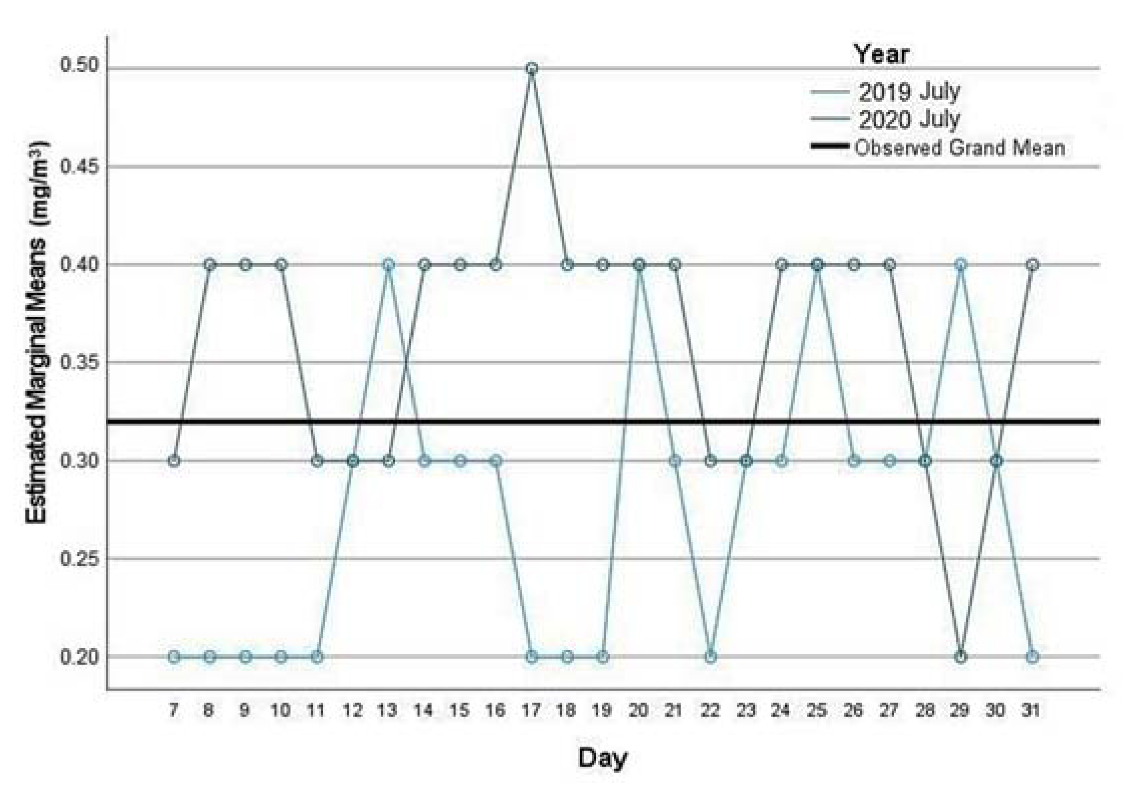
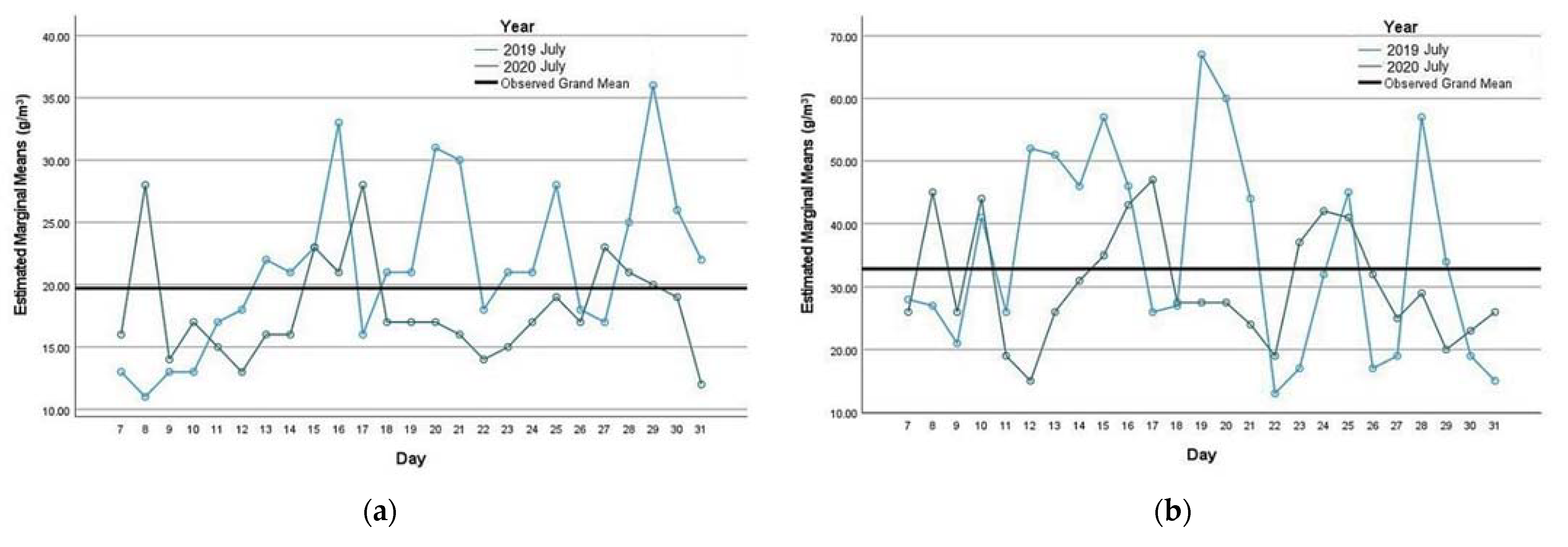
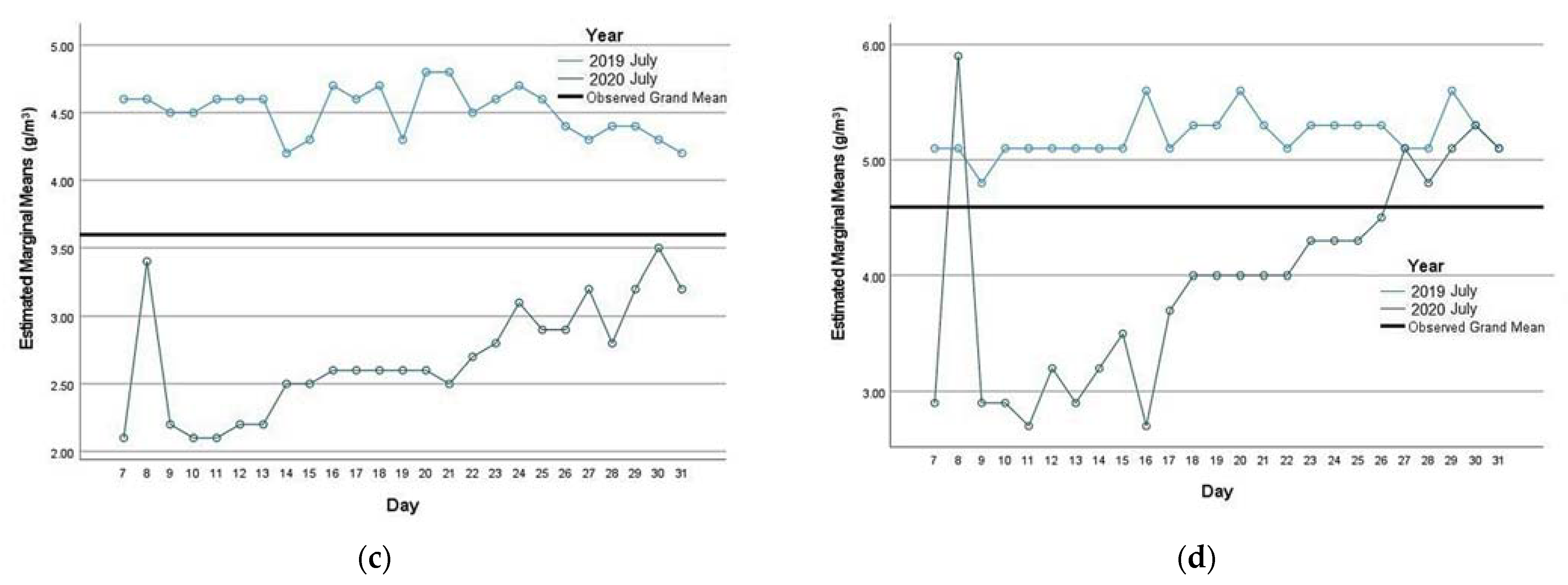
Comparative data analysis results showed that the situation had changed and that the amounts of some pollutants (PM10 and NO2), as measured by the Automatic Air Quality testing station, had decreased (see Table 3). Despite the fact that the solution of loop traffic changed the habits of many residents who visited Vilnius Old Town, the average CO concentration in this zone did not reduce. On the contrary, the value increased from 0.276 µg/m3 in 2019 to 0.364 µg/m3 in 2020 (p < 0.01, ∆ = −0.09, Table 3). Additionally, we identified that some of the pollutant values statistically significant decreased: amounts of PM10 (p < 0.01, ∆ = 3.36), SO2_1 h (p < 0.01, ∆ = 1.83), and SO2_24 h (p < 0.01, ∆ = 1.24) in July 2020 (Table 3). We analysed a significant interaction effect between measurement year and day. The significant differences between 7–31 July 2019 and 7–31 July 2020 pollution were identified for PM10 (p < 0.05, ηp2 = 0.44) (see Table 3). The PM10 amounts were significantly higher (p < 0.05) in 7–31 July 2019 (Table 3). In addition, an interaction effect (p < 0.05) between day and year was obtained on PM10, CO, SO2_1 h, SO2_24 h (g/m3) and NO2 (g/m3). The estimated PM10, SO2_1 h and SO2_24 h were higher 7–31 July 2019 than 7–31 July 2020 (p < 0.05, ηp2 = 0.72, 0.61, 0.75) throughout the day measurement. However, no significant differences of air contamination by NO2 between conditions in 7–31 July 2019 and 7–31 July 2020 were found (Table 3). Despite this, the size of the mean differences of NO2 was small. Finally, all 0of the variables showed a significant decrease over 7–31 July 2019 (p < 0.05, ηp2 = 0.52–0.97) with 1 exception for CO (Table 3 and Figure 5 and Figure 6).

4.3. Inferential Statistical Analysis Results

The multi-perceptron neural networks were chosen for dataset analysis to answer the research questions. Following to the specificity of the neural network analysis, the dataset was divided into different partition rates and then assigned training, testing, and holdout conditions: MLPN1 = 40%-40%-20%, MLPN2 = 50%-30%-20%, and MLPN3 = 60%-20%-20%. This analysis allowed us to validate the model under different conditions. Furthermore, the model was designed using specific parameters: initial lambda, which was set to 0.0000005; initial sigma, which was set to 0.00005; interval centre (ao and a) forced the simulated annealing algorithm to generate random weights between (ao − a) and (ao + a) to minimize the error function and interval centre as well as the interval offset. Moreover, 0 was defined as the interval centre, and the interval offset was set to ±0.5.

Results of Case Processing

The multilayer perceptron neural network was used to help correctly predict air pollution before and after implementing the loop traffic agreement. Table 3 presents descriptive statistical information about the datasets used to design the neural network models.
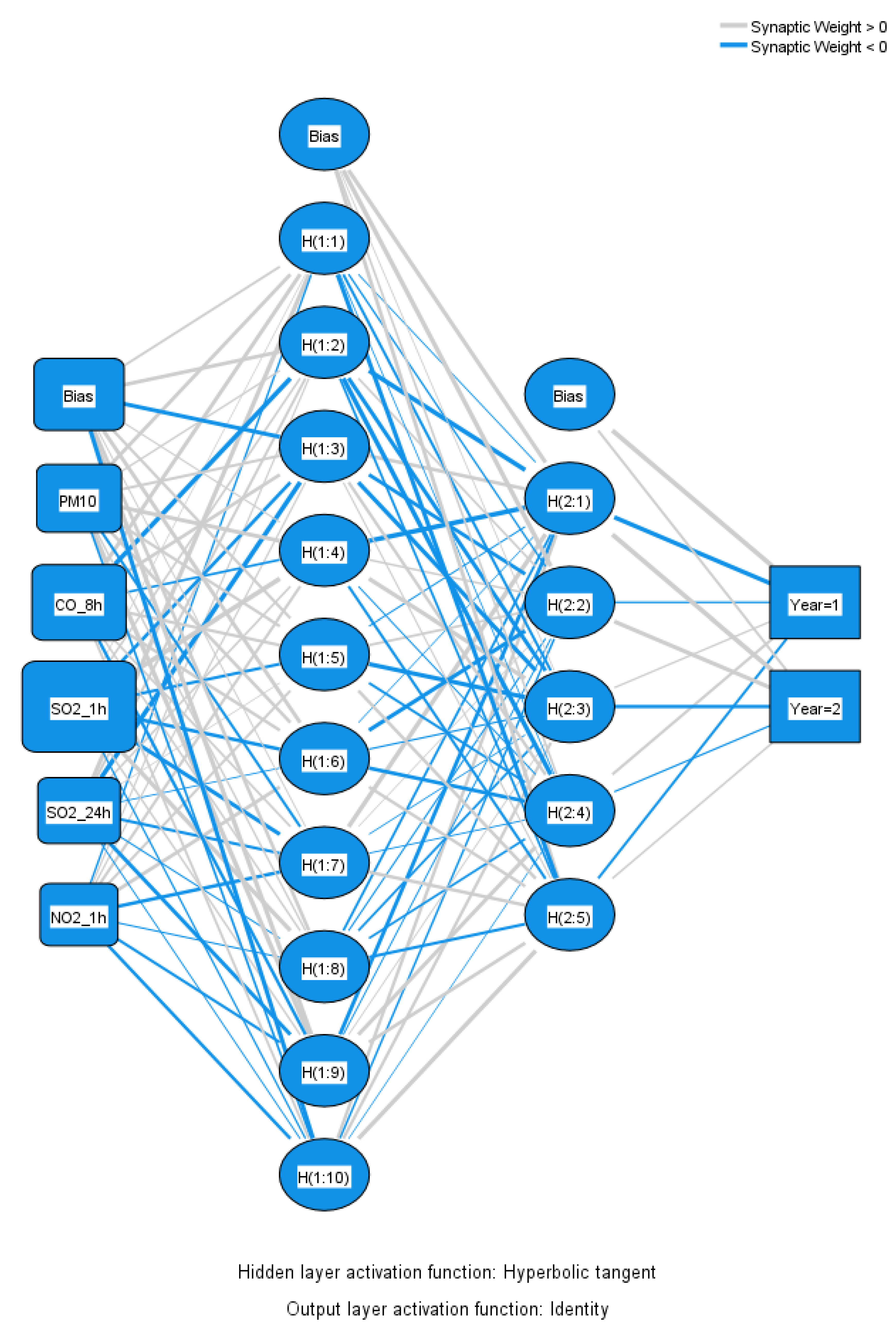
We used custom architecture for the MLPN network design with ten nodes for the first hidden layer, five nodes for the second hidden layer, and two for the output layer computations. Hyperbolic tangent activation function was used for the hidden layers, and identity function was used for the output layer. Validation of the constructed models was evaluated by the sum of square function (see Table 4).
The high validated network (MLPN1) diagram is shown in Figure A1 (Appendix B), which illustrates the diagram with 5 input nodes, 15 hidden nodes, and 2 output nodes according to the 2 dependent variable categories. The summary for the designed models provides information on the results of the training (and testing) and holdout sample, as shown in Table 5.
The sum of squares error was used for both the training and testing samples. The MLPN1 (4-4-2) model was identified as having the smallest sum of squares error value (training = 0.005; testing = 0.021), indicating the model’s capability to predict air pollution before the introduction of loop traffic (July 2019) and after (July 2020).
According to the calculation results, the MLPN1 model’s percentages of inappropriate predictions constructed on the training and testing samples were 0.0% and 0.0%, respectively. Moreover, the degree of improper predictions in the holdout dataset equalled 0.0%. The training procedure was performed until one consecutive step with no decrease in the error function was achieved. Additionally, the synaptic weights of MLPN1 (40%-40%-20%) are presented in Supplementary Materials as Table S1.
The outcome in Table 6 for the MLPN1 model demonstrates that 20 cases (out of 20) of air quality situations were classified correctly and measured by the 2 categories in the training data sample and 20 out of 20 variables in the testing sample. Overall, the designed model MLPN1 properly classified 100.0% of the training and testing cases. The same situation appears for the MLPN2 model.
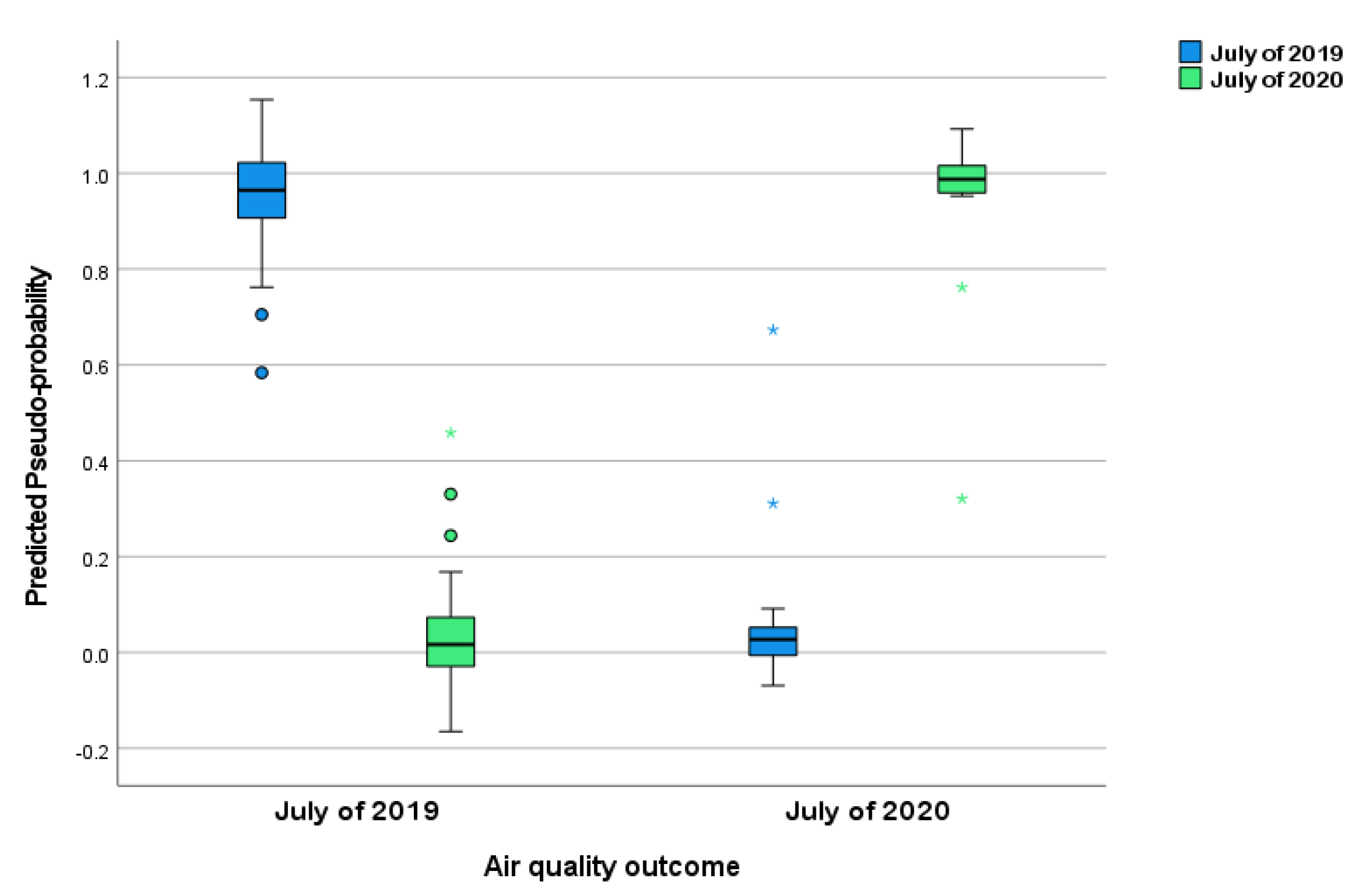
Additionally, the MLPN1 model’s predicted pseudo-probability for the two situations of air quality categories of the SIT variable are presented in a box-plot diagram (see Figure 7).
This specific graph separately illustrated the predictions for the two categories of the dependent variable SIT and categorized the predicted pseudo-probabilities based on the whole analysed dataset. Detailed analysis of the diagram should start from the left side. The first boxplot on the left shows the predicted probability of the observed situation of air conditions in the category before the loop traffic agreement (July 2019) in the Vilnius Old Town. The second boxplot shows the probability for air conditions classified in the category after the loop traffic agreement (July 2020). The third boxplot shows the outcomes that have been observed in the category after the loop traffic agreement (July 2020) and the predicted probability of the category before the loop traffic agreement (July 2019). The right boxplot shows the probability for air conditions that succeeded to be classified in the category after the loop traffic agreement (July 2020).
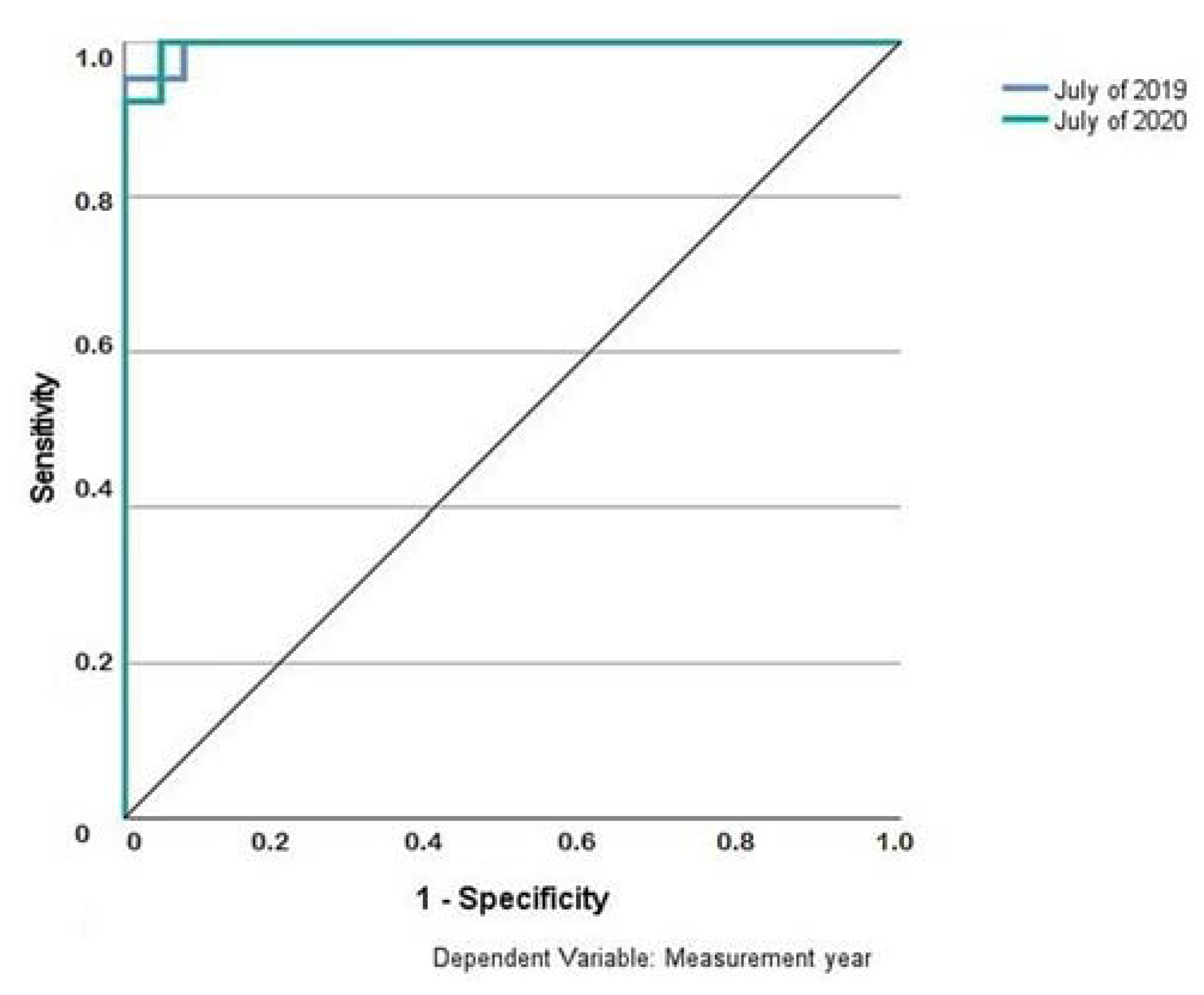
Moreover, the MLPN1 model was validated using the ROC curve, which showed the classification performance for all possible cut-offs in the sensitivity versus specificity diagram (Figure 8).
In this model, the research dataset was divided in the following way to be analysed: training = 40%, testing = 40%, and holdout = 20%. Figure 8 gives the sensitivity and specificity (situation in July 2019 and July 2020) diagram constructed on the training and testing illustrations. The 45-degree line from the lower-left corner to the upper right corner of the chart characterizes the situation of randomly guessing the category. The further the curve moves from the 45-degree reference line, the more precise the classification. The area under the curve (AUC) was measured, and the higher validation result of 1.000 as an AUC appeared for the air quality category SIT1 and 0.998 for the category SIT2 (see Table 7).
Measures of sensitivity and specificity for the designed MLPN1, MLPN2, and MLPN3 models were presented as the AUC, which presents the entire position of the ROC curve according to the SIT variable’s 2 categories: July 2019 and July 2020. The AUC presented in Table 7 can be described as the probability of a randomly selected air condition situation being rated or ranked correctly. This explanation is based on non-parametric Mann–Whitney U statistics. Moreover, the maximum AUC = 1.000 (MLPN1, SIT group 2 = July 2020, Table 7) showed that air conditions assessed using the recorded values of pollutants as air pollution markers demonstrated a high predictive ability to classify situations before and after the loop traffic agreement.
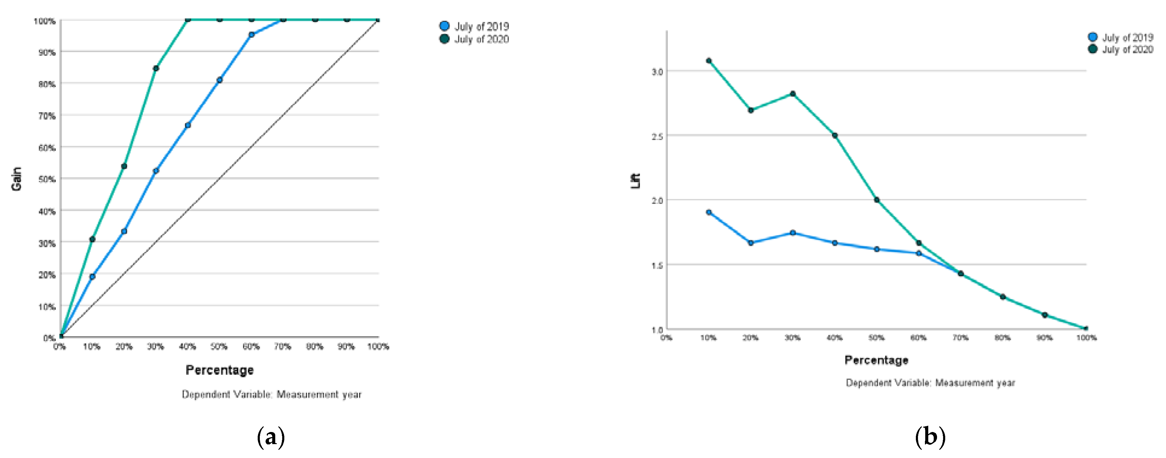
The chart in Figure 9a provides the cumulative gains that illustrate the accurate classifications gained by the MLPN1 model against the correct classifications that could affect by chance (without exploiting the model). The gains chart demonstrates the success of the classification designed by the neural network model. For example, the third point on the curve for the category that presents air conditions after the loop traffic agreement (July 2020) is at (30%, 85%). This can be explained in terms of the network scoring the data and classifying all air quality conditions using the predicted pseudo-probability of the category after the loop traffic agreement. The top 30% is predicted to cover approximately 85% of all cases in the situation described by the second SIT category (July 2020). It is not significant to select 100% of the scored data to find all of the recognized illustrations of air quality established in the dataset. Accordingly, the higher overall gain specifies higher performance. Additionally, Figure 9b helps to graphically judge the performance of the classification models. Moreover, the presented lift graph, which uses a portion of the dataset, can show a clear view of the benefit of the modelling result, if not using modelling. The values from the gains diagram were used to compute the lift feature (i.e., the support): the lift at 100% for the second SIT category (July 2020) was 85%/30% = 2.8.
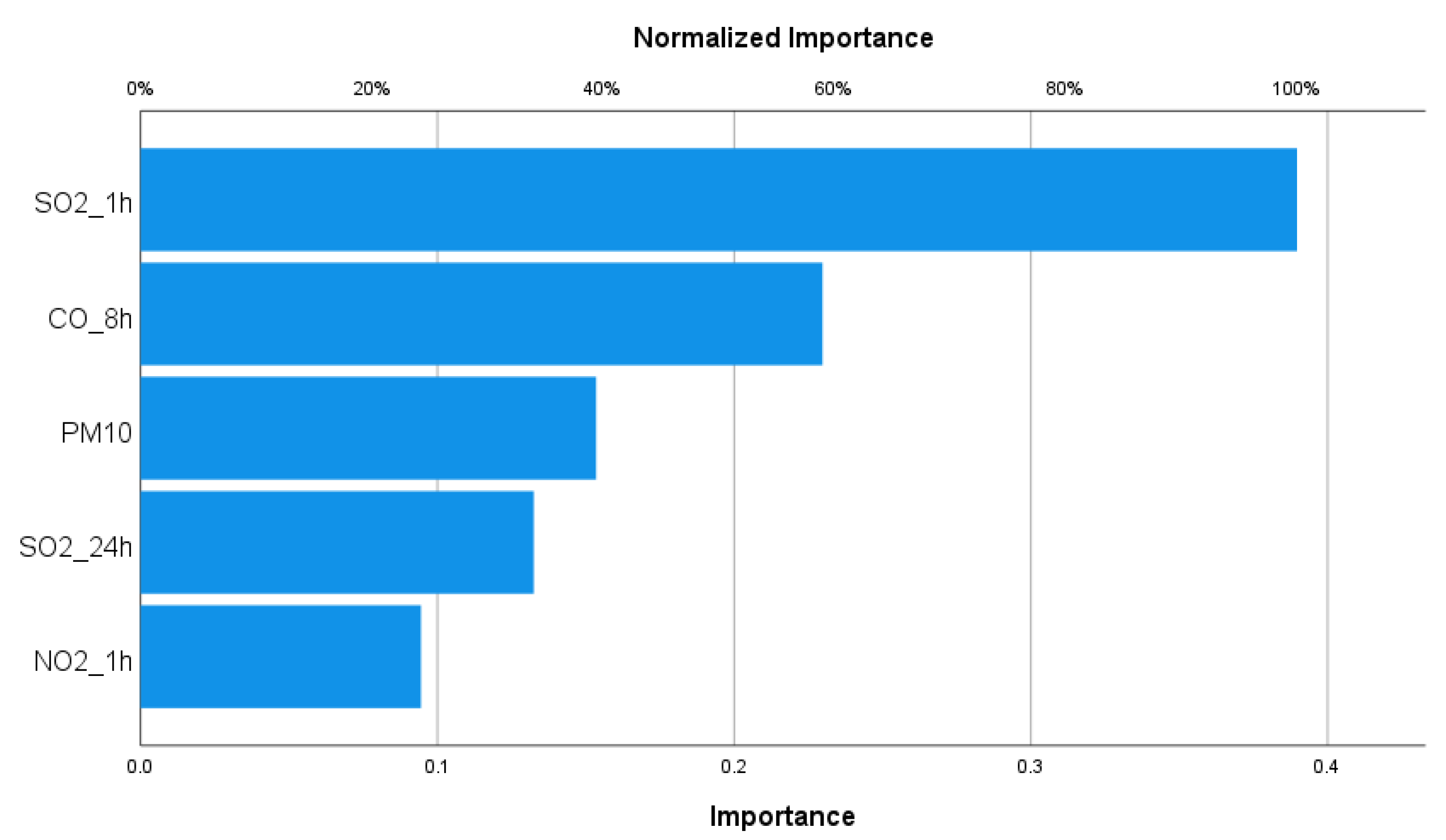
Furthermore, the impact of each pollutant on air quality predictions in terms of relative and normalized importance acknowledged in the models MLPN1, MLPN2, and MLPN3 is demonstrated in Table 8. We found that the variable SO2_1 h had the highest importance of all predictors (normalized importance = 100%). The highest normalized importance of air quality prediction was identified for the maximum concentration of sulphur dioxide per one hour (SO2_1 h, g/m3) in all constructed MLPN models (Table 8). In addition, the chart for the MLPN1 model is presented for a better illustration of the pollutants and their importance for air contamination increases (see Figure A1 and Figure A2, Appendix B).

5. Discussion and Limitations

On 7 July 2020, Vilnius Old Town embraced traffic changes, whereby the regulation of loop traffic was introduced to the area. Visitors and residents of the Old Town could continue to drive to their homes, workplaces, and attractions. However, many drivers were no longer able to cross the Old Town in order to shorten their journey time. The introduction of loop traffic aimed to improve the quality of life of the residents of the Old Town. Reducing vehicle traffic meant that noise and air pollution also diminished. However, the changes affected the public transport system so that both the residents and the guests of the capital were able to travel by conventional bus routes. Consequently, it was important to assess the changes in air quality after the loop traffic agreement.
The study analysed a dataset from 2018 to 2020 as recorded by the Automatic Air Quality testing stations in the Vilnius agglomeration. The research was conducted to help and identify air quality in the Vilnius agglomeration and the area of Vilnius Old Town. Based on the collected air quality dataset, these investigations included a control component, which was the dependent variable SIT (1 = July 2019, 2 = July 2020), air pollution in the Vilnius Old Town in 2 different situations (after and before the loop traffic agreement), and five independent variables: PM10, CO, SO2_1 h, SO2_24 h, and NO2, which were chosen to investigate how loop traffic helps to reduce air pollution in the Old Town area of Vilnius.
Particulate matter is a mixture of airborne particles and liquid droplets, also known as aerosols, which actively absorb toxic substances and microorganisms and carry hazardous substances. In addition, the finer the particles, the deeper they penetrate the human body and, in turn, the greater their adverse effects on human health. Accordingly, we focused on the amount variations of this pollutant in the Vilnius agglomeration. The results in terms of the annual average daily concentrations of particulates under 10 microns in diameter (PM10, g/m3) showed that PM10 changed the least in the Vilnius Old Town: they ranged from 28 µg/m3 (2018) to 26 µg/m3 (2019); in 2020, they were recorded at 24 µg/m3. Therefore, the annular data investigations for the number of days when the recorded daily limit value for PM10 (50 µg/m3) was exceeded in 2018–2020 showed that extreme values of PM10 were recorded ten times days as in 2019 as in the 2020 year. These findings proved the same problem with the heavy traffic loads, and it is along the same lines as those of other scholars [64,65,66], who identified that air pollution caused by PM is one of the most pressing problems in cities. The most common sources of particulate pollution are vehicles, combustion processes (heat production, fires, scrap), industrial activities, etc. [65,67,68]. This led us to reach a similar conclusion to other scholars [64,69] that the most common sources of particulate pollution sources were frequently localized as depicted by high concentrations at low wind speeds in the area of Vilnius Old Town, mostly by the emissions from road vehicles that increased pollution in the summertime (July) due to the unfavourable dispersal conditions.
Carbon monoxide (CO) is an odourless, colourless, and highly toxic gas formed during the combustion process when the combustible materials are not fully oxidized. The maximum concentrations of CO (CO = 0.50 mg/m3) per 1 hour was registered in July 2020. Student t-test is statistically significantly higher than in July 2019 (CO = 0.40 mg/m3). This is a worrying outcome because it proves that vehicles are one of the main sources of carbon monoxide formation in the summertime in the Vilnius Old Town. This finding is concurrent with other research into air pollution in cities [67,70,71].
When analysing the neural network modelling results, the highest normalized importance (normalized importance = 100%) of air quality prediction was found with the maximum concentration of sulphur dioxide per one hour (SO2_1 h, g/m3). Moreover, SO2_1 h pollutant had the highest indication (normalized importance = 100%) in all of the constructed neural network models to judge the importance of independent variables. Another predictor with high importance was carbon monoxide (mg/m3), indicated by the maximum concentrations of carbon monoxide per one hour (normalized importance = 59.0%, MLPN1). Next in importance was PM10 (normalized importance = 39.4%, MLPN1). Unexpectedly, nitrogen dioxide (NO2), a pollutant attributable to the transport sector, was found to have a small impact (normalized importance = 24.2%, MLPN1) on air pollution in the Old Town. This importance varied across the different models (see Table 8). The multilayer perceptron neural networks design with custom architecture with hyperbolic tangent activation function for two hidden layers (ten nodes for the first hidden layer and five nodes for the second) and identity function for the output layer computations were validated in the same way as other scholars did by the sum of square function [24,48,49,50,51,52,53,54,55]. The research findings demonstrate that the highest accuracy was reached with the MLPN1 with 4-4-2 partition, the standardized rescaling method for covariates, and the backpropagation algorithm. MLPN1 model was acknowledged as the best by the smallest sum of square error value of 0.005, a correct classification rate of 100%, and the AUC for each category with the predicted pseudo-probability (July 2019 = 0.997; July 2020 = 1.000).
The specific location area of AQC stations enabled us to conduct the comparative data analysis and assess the average annual particulate matter PM10 in the Vilnius agglomeration. We identified that PM10 in 2018 ranged from 13 to 36 µg/m3 and from 13 to 24 µg/m3 in 2020 and did not exceed the limit value (40 µg/m3). In addition, a higher CO concentration was identified in the Vilnius Old Town AQC station in 2018 (3.5 mg/m3). However, the CO concentration decreased later. In 2019, the average CO concentration was 2.1 mg/m3, and in 2020–1.4 mg/m3. Moreover, although Lazdynai AQC station is located in a residential area, away from streets and other sources of pollution, the maximum daily concentration of sulphur dioxide (SO2) was recorded in Lazdynai AQC station from 2018 to 2020.
This study has limitations. Firstly, the research design was based on a dataset from 2018–2020. Secondly, air conditions in the Vilnius agglomeration were measured without including meteorological parameters, which play a key role in the moderation or intensification of air pollution. Thirdly, this analysis did not investigate the correlation between daily changes in pollution and changes in human health in the Vilnius agglomeration. It can also be assumed that all of the components of the air quality control process must be fair to avoid offsetting effects between the components. Given the above caveats, the study’s conclusions must be interpreted carefully.
Future research can include variables such as minimum and maximum daily temperature, average daily temperature, total daily rainfall, sunny hours, cloudy hours, maximum daily wind speed, wind direction, average wind speed, maximum and minimum humidity measures, which have been considered in other studies [10,28]. Additionally, air quality assessment studies can include the statistical measures of daily vehicle traffic in the city and noise indicators [72]. Despite these limitations, this study used accurate methods to predict air pollution and provided interesting evidence regarding the role of the loop traffic agreement in the Vilnius Old Town. Consequently, the prediction of air pollutants based on the modelling of neural networks could significantly contribute to the decision-making of Vilnius city managers and planners as it concerns the negative effects of air pollution.

6. Conclusions

This scientific work has been conducted to gain more knowledge and new evidence regarding air quality in the Vilnius agglomeration after an internal integrated city transport corridor was formed, built Vilnius Southern Bypass and Vilnius Western Bypass, and the regulation of loop traffic was introduced.
The chosen analysis methods helped to identify the main pollutants that cause the most air pollution and aggravate human health problems. The offered air contamination assessment has 4 important aspects which make it different from those which have been previously presented: (1) our analysis focuses on the interaction between air pollution and assessment of the impact of the proposed transport policies has on urban sustainability in Vilnius Old Town strategy rather than assuming that the strategies are simply independent; (2) our data modelling takes into account that air pollution is a multidimensional phenomenon that must be measured and modelled using nonlinear methods, which is ignored in the pollution assessment dynamics literature; (3) Mathematically, artificial neural network modelling is used in purpose to handle complex systems with many interrelated parameters; (4) the new evolutionary-based algorithm was developed by simultaneously changing the topology and the connection weights of ANNs by means of different combinations of genetic algorithm. Furthermore, the results of this study will contribute to the planning of ambient air quality management in the Vilnius agglomeration. This research will help make the right decisions in maintaining healthy air quality concerning human health and the environment. When preparing a plan for air quality management, it is necessary to assess ambient air pollution and identify and evaluate the main pollutants that contribute to the level of ambient air pollution. Accurate methods for predicting air pollution can help find insights for solutions to reduce air pollution in the Vilnius agglomeration. Therefore, the prediction of air pollutants based on a dataset recorded by the Automatic Air Quality testing stations could largely contribute to the decision-making of city managers and planners as it concerns the adverse effects of air pollution on Vilnius Old Town.
Future studies on complex air pollution modelling should focus on the indicators or multifaceted methods that may better reflect the way pollutants cause air pollution and influence health. Despite the findings of the investigation that demonstrated effective implementation of neural network modelling for air pollution, future studies need to validate these findings with extended datasets. In addition, future studies could be extended by research into the correlation between daily changes in pollution and changes in health. Furthermore, this type of analysis could consider other contributing factors, such as the season, temperature, and the day of the week.

Supplementary Materials

The data supporting the reported results are available online at https://www.mdpi.com/article/10.3390/su14042470/s1, Table S1_ synaptic weights of MLPN1.xlsx.

Author Contributions

Conceptualization, S.B. and I.M.-K.; methodology, S.B. and I.M.-K.; software, S.B.; validation, S.B.; formal analysis, S.B.; investigation, S.B.; resources, S.B. and I.M.-K.; data curation, S.B.; writing—original draft preparation, S.B. and I.M.-K.; writing—review and editing, S.B. and I.M.-K.; visualization, S.B.; supervision, I.M.-K.; project administration, S.B. and I.M.-K.; funding acquisition, S.B. and I.M.-K. All authors have read and agreed to the published version of the manuscript.

Funding

This research was funded by Ministry of National Defence Republic of Lithuania as a part of the research project Study Support Projects No VI-18, 2 December 2021 (2021–2024), General Jonas Žemaitis, Military Academy of Lithuania, Vilnius, Lithuania. Any opinions, findings and conclusions or recommendations expressed in this material are those of the authors and do not necessarily reflect the view of the funding agency.

Institutional Review Board Statement

The study was conducted according to the guidelines of the Declaration of Helsinki.

Informed Consent Statement

This research there were not used specifically human materials.

Data Availability Statement

The data of this study is available from the authors upon request.

Conflicts of Interest

The authors declare no conflict of interest.

Appendix A

Table A1. Types of Automatic Air Quality testing stations employed in the Vilnius agglomeration.
1 StationStation TypeStation CoordinatesDescription
Vilnius, Old Towncity backgroundN 54°40′53″ E 25°17′17″Located in a densely populated, crowded area, near a low-traffic street.
Vilnius, Lazdynaicity backgroundN 54°41′8″ E 25°12′39″ Located in a residential area, away from streets and other sources of pollution.
Vilnius, ŽirmūnaitransportN 54°42′55″ E 25°17′22″Located close to heavy traffic on Kareivių Street, near the intersection with Kalvarijų Street.
Vilnius, Savanorių AvenueindustrialN 54°40′24″ E 25°14′56″Located on a busy street, but at a greater distance from it, in a square next to residential houses. Air quality in this area can be significantly affected by emissions from both transport and the nearby industrial and energy companies in Žemieji Paneriai.
Notes: 1 Vilnius agglomeration, Lithuania.
Table A2. Aggregate statistical indicators of air quality in the Vilnius agglomeration in the period of 2019–2020.
StationPM10
µg/m3
PM2.5
µg/m3
SO2
µg/m3
NO2
mg/m3
O3
µg/m3
CO
mg/m3
C6H6
µg/m3
CvidCmax 24 hPCvidCvidCmax 24 hCmax
1 h
CvidCmax
1 h
VCmax
8 h
P1P2Cmax
1 h
Cmax
8 h
Cvid
2020 Existing Standards, Limit Values, Information and Alert Thresholds for the Protection of Human Health
405035 d.20 1253504020018120 (1) 25
Vilnius Old Town2415510 5.99.513.3151090 1.4
Vilnius, Lazdynai251496 10.115.022.61195011703124
Vilnius, Žirmūnai271521613.6 251230117021270.90.23 *
Vilnius, Savanorių Avenue131406 5.010.038.614870 1.20.38 *
2019 existing standards, limit values, information and alert thresholds for the protection of human health
Station405035 d.20 1253504020018120 (1) 25
Vilnius Old Town268710 5.88.943.9181040 2.1
Vilnius, Lazdynai17623 4.717.234.11179014393147
Vilnius, Žirmūnai30801516 311200149521541.40.24 *
Vilnius, Savanorių Avenue198210 5.09.125.8181480 1.10.29 *
Notes: Cvid–average annual concentration; Cmax 24 h–maximum daily concentration; Cmax 1 h–maximum 1 h. concentration; Cmax 8 h–maximum 8 h. Concentration for the period is calculated using the moving average method; 120 (1)–the target value for ozone must not be exceeded for more than 25 days in a year, averaged over 3 years. P–number of days when the daily limit value was exceeded (50 µg/m3); P1–number of days when 8 h were exceeded. Ozone target value for 2019; P2–average annual number of days when the limit value in the 8 h period was exceeded. Target value for ozone, 2018–2020; V–number of hours when the limit value in the 1 h period was exceeded. Limit value (200 µg/m3); *–less than 90% of data collected.

Appendix B

Figure A1. Predicted normalized importance for pollutants according to the MLPN1 (40%-20%-20%) model.
Sustainability 14 02470 g0a1
Figure A2. MLPN1 topology for cycle time with multi-layered perceptron.
Sustainability 14 02470 g0a2

References

  1. Republic of Lithuania Law on Environmental Protection. Available online: https://e-seimas.lrs.lt/portal/legalAct/lt/TAD/6378f2b0023211e6bf4ee4a6d3cdb874 (accessed on 3 May 2021).
  2. Review of the National Air Pollution Control Programme. Available online: https://ec.europa.eu/environment/air/pdf/reduction_napcp/NAPCP%20review%20report%20LT%20-%20Final%20updated%2025Jun20.pdf (accessed on 3 May 2021).
  3. Guarnieri, M.; Balmes, J.R. Outdoor air pollution and asthma. Lancet 2014, 383, 1581–1592. [Google Scholar] [CrossRef] [Green Version]
  4. Frosina, E.; Romagnuolo, L.; Bonavolontà, A.; Andreozzi, A.; Senatore, A.; Fortunato, F.; Giliberti, P. Evaporative emissions in a fuel tank of vehicles: Numerical and experimental approaches. Energy Procedia 2018, 148, 1167–1174. [Google Scholar] [CrossRef]
  5. Nieuwenhuijsen, M.J. Urban and transport planning, environmental exposures and health-new concepts, methods and tools to improve health in cities. Environ. Health 2016, 15, 38. [Google Scholar] [CrossRef] [PubMed] [Green Version]
  6. Bigazzi, A.Y.; Rouleau, M. Can traffic management strategies improve urban air quality? A review of the evidence. J. Transp. Health 2017, 7 Pt B, 111–124. [Google Scholar] [CrossRef]
  7. Bradley, N.; Dobney, A.; Exley, K.; Stewart-Evans, J.; Aldridge, S.; Craswell, A.; Dimitroulopoulou, S.; Hodgson, G.; Izon-Cooper, L.; Mitchem, L.; et al. Review of Interventions to Improve Outdoor Air Quality and Public Health. 2019. Available online: https://www.gov.uk/government/publications/improving-outdoorair-quality-and-health-review-of-interventions (accessed on 3 May 2021).
  8. Burns, J.; Boogaard, H.; Polus, S.; Pfadenhauer, L.M.; Rohwer, A.C.; van Erp, A.M.; Turley, R.; Rehfuess, E. Interventions to reduce ambient particulate matter air pollution and their effect on health. Cochrane Database Syst. Rev. 2019, 5, CD010919. [Google Scholar] [CrossRef]
  9. Conlan, B.; Fraser, A.; Vedrenne, M.; Tate, J.; Whittles, A. Evidence Review on Effectiveness of Transport Measures in Reducing Nitrogen Dioxide: Exploring and Apprasing Proposed Measures to Tackle Air Quality, Department for Environment Food and Rural Affairs. 2016. Available online: https://uk-air.defra.gov.uk/assets/documents/reports/cat05/1605120947_AQ0959_appendix_1-evidence_review_on_air_quality_effects_of_transport_measures.pdf (accessed on 3 May 2021).
  10. Holman, C.; Harrison, R.; Querol, X. Review of the efficacy of low emission zones to improve urban air quality in European cities. Atmos. Environ. 2015, 111, 161–169. [Google Scholar] [CrossRef]
  11. Amsterdam Climate Neutral 2050 Roadmap-Phase 1: An Invitation to the City. Available online: http://carbonneutralcities.org/wp-content/uploads/2019/12/Amsterdam-Climate-Neutral-2050-Roadmap_12072019-1.pdf (accessed on 3 May 2021).
  12. Gurjar, B.R.; Butler, T.M.; Lawrence, M.G.; Lelieveld, J. Evaluation of emissions and air quality in megacities. Atmos. Environ. 2008, 42, 1593–1606. [Google Scholar] [CrossRef]
  13. Manucci, P.M.; Franchini, M. Health effects of ambient air pollution in developing countries. Int. J. Environ. Res. Public Health 2017, 14, 1048. [Google Scholar] [CrossRef]
  14. WHO. Air Pollution. Available online: http://www.who.int/airpollution/en/ (accessed on 5 June 2021).
  15. Ali, M.; Athar, M. Air pollution due to traffic, air quality monitoring along three sections of National Highway N-5, Pakistan. Environ. Monit. Assess. 2008, 136, 219–226. [Google Scholar] [CrossRef]
  16. Aziz, A.; Bajwa, I.U. Minimizing human health effects of urban air pollution through quantification and control of motor vehicular carbon monoxide (CO) in Lahore. Environ. Monit. Assess. 2007, 135, 459–464. [Google Scholar] [CrossRef]
  17. Reikard, G. Volcanic emissions and air pollution: Forecasts from time series models. Atmos. Environ. X 2019, 1, 100001. [Google Scholar] [CrossRef]
  18. Rybarczyk, Y.; Zalakeviciute, R.; Rybarczyk, Y.; Zalakeviciute, R. Machine Learning Approaches for Outdoor Air Quality Modelling: A Systematic Review. Appl. Sci. 2018, 8, 2570. [Google Scholar] [CrossRef] [Green Version]
  19. Kumar, A.; Goyal, P. Forecasting of air quality in Delhi using principal component regression technique. Atmos. Pollut. Res. 2011, 2, 436–444. [Google Scholar] [CrossRef] [Green Version]
  20. Donnelly, A.; Misstear, B.; Broderick, B. Real time air quality forecasting using integrated parametric and non-parametric regression techniques. Atmos. Environ. 2015, 103, 53–65. [Google Scholar] [CrossRef]
  21. Zhu, J.; Wu, P.; Chen, H.; Zhou, L.; Tao, Z.; Zhu, J.; Wu, P.; Chen, H.; Zhou, L.; Tao, Z. A Hybrid Forecasting Approach to Air Quality Time Series Based on Endpoint Condition and Combined Forecasting Model. Int. J. Environ. Res. Public Health 2018, 15, 1941. [Google Scholar] [CrossRef] [Green Version]
  22. Silibello, C.; D’Allura, A.; Finardi, S.; Bolignano, A.; Sozzi, R. Application of bias adjustment techniques to improve air quality forecasts. Atmos. Pollut. Res. 2015, 6, 928–938. [Google Scholar] [CrossRef]
  23. Sozzi, R.; Bolignano, A.; Ceradini, S.; Morelli, M.; Petenko, I.; Argentini, S. Quality control and gap-filling of PM10 daily mean concentrations with the best linear unbiased estimator. Environ. Monit. Assess. 2017, 189, 562. [Google Scholar] [CrossRef]
  24. Bekesiene, S.; Meidute-Kavaliauskiene, I.; Vasiliauskiene, V. Accurate Prediction of Concentration Changes in Ozone as an Air Pollutant by Multiple Linear Regression and Artificial Neural Networks. Mathematics 2021, 9, 356. [Google Scholar] [CrossRef]
  25. Radojevi´c, D.; Antanasijevi´c, D.; Peri´c-Gruji´c, A.; Risti´c, M.; Pocajt, V. The significance of periodic parameters for ANN modeling of daily SO2 and NOx concentrations: A case study of Belgrade, Serbia. Atmos. Pollut. Res. 2019, 10, 621–628. [Google Scholar] [CrossRef]
  26. Pawlak, I.; Jarosławski, J.; Pawlak, I.; Jarosławski, J. Forecasting of Surface Ozone Concentration by Using Artificial Neural Networks in Rural and Urban Areas in Central Poland. Atmosphere 2019, 10, 52. [Google Scholar] [CrossRef] [Green Version]
  27. Biancofiore, F.; Busilacchio, M.; Verdecchia, M.; Tomassetti, B.; Aruffo, E.; Bianco, S.; Di Tommaso, S.; Colangeli, C.; Rosatelli, G.; Di Carlo, P. Recursive neural network model for analysis and forecast of PM10 and PM2.5. Atmos. Pollut. Res. 2017, 8, 652–659. [Google Scholar] [CrossRef]
  28. James, K.L.; Randall, N.P.; Haddaway, N.R. A methodology for systematic mapping in environmental sciences. Environ. Evid. 2016, 5, 7. [Google Scholar] [CrossRef] [Green Version]
  29. Samet, J.M.; Dominici, F.; Zeger, S.L.; Schwartz, J.; Dockery, D.W. The National Morbidity, Mortality, and Air Pollution Study. Part I: Methods and methodologic issues. Res. Rep. Health Eff. Inst. 2000, 94, 5–14; discussion 75–84. [Google Scholar] [PubMed]
  30. Katsouyanni, K.; Touloumi, G.; Samoli, E.; Gryparis, A.; Le Tertre, A.; Monopolis, Y.; Rossi, G.; Zmirou, D.; Ballester, F.; Boumghar, A.; et al. Confounding and effect modification in the short-term effects of ambient particles on total mortality: Results from 29 European cities within the APHEA2 project. Epidemiology 2001, 12, 521–531. [Google Scholar] [CrossRef] [Green Version]
  31. Dominici, F.; Daniels, M.; Zeger, S.L.; Samet, J.M. Air pollution and mortality: Estimating regional and national dose-response relationships. J. Am. Stat. Assoc. 2002, 97, 100–111. [Google Scholar] [CrossRef]
  32. Anderson, H.R.; Atkinson, R.W.; Peacock, J.L.; Sweeting, M.J.; Marston, L. Ambient particulate matter and health effects: Publication bias in studies of short-term associations. Epidemiology 2005, 16, 155–163. [Google Scholar] [CrossRef]
  33. Le Tertre, A.; Medina, S.; Samoli, E.; Forsberg, B.; Michelozzi, P.; Boumghar, A. Short-term effects of particulate air pollution on cardiovascular diseases in eight European cities. J. Epidemiol. Commun. Health 2002, 56, 773–779. [Google Scholar] [CrossRef]
  34. Zhang, Y.; Ma, Y.; Feng, F.; Cheng, B.; Wang, H.; Shen, J.; Jiao, H. Association between PM10 and specific circulatory system diseases in China. Sci. Rep. 2021, 11, 12129. [Google Scholar] [CrossRef]
  35. Wu, T.; Ma, Y.; Wu, X.; Bai, M.; Peng, Y.; Cai, W.; Wang, Y.; Zhao, J.; Zhang, Z. Association between particulate matter air pollution and cardiovascular disease mortality in Lanzhou, China. Environ. Sci. Pollut. Res. Int. 2019, 26, 15262–15272. [Google Scholar] [CrossRef]
  36. El Shawarby, I.; Kyoungho, A.; Hesham, R. Comparative field evaluation of vehicle cruise speed and acceleration level impacts on hot stabilized emissions, Transportation Research Part D. Transp. Environ. 2005, 10, 13–30. [Google Scholar] [CrossRef]
  37. Lawson, D.R. Passing the Test-Human Behavior and California’s Smog Check Program. J. Air Waste Manag. Assoc. 1993, 43, 1567. [Google Scholar] [CrossRef] [Green Version]
  38. Kazopoulo, M.; El Fadel, M.; Kaysi, I. Emission standards development for an inspection/maintenance program. J. Environ. Eng. 2005, 131, 1330–1339. [Google Scholar] [CrossRef]
  39. Levinson, D.M.; Gillen, D.; Kanafani, A. The social costs of intercity transportation: A review and comparison of air and highway. Transp. Rev. 1998, 18, 215–240. [Google Scholar] [CrossRef]
  40. World Health Organization. World Health Organization, 2018. Global Air Pollution Issue. Available online: https://www.who.int/airpollution/infographics/en/ (accessed on 3 May 2021).
  41. USEPA. Guidelines for Carcinogen Risk Assessment Review Draft. NCEA-F-0644. July 1999. Available online: http://www.epa.gov/cancerguidelines/draft-guidelines-carcinogen-ra-1999.htm (accessed on 23 January 2021).
  42. Oak Ridge National Laboratory. Available online: https://www.ornl.gov/sites/default/files/ORNL%20Review%20v33n3%202000.pdf (accessed on 23 January 2021).
  43. Slovic, A.D.; de Oliveira, M.A.; Biehl, J.; Ribeiro, H. How can urban policies improve air quality and help mitigate global climate change: A systematic mapping review. J. Urban Health 2016, 93, 73–95. [Google Scholar] [CrossRef] [Green Version]
  44. Stieb, D.M.; Judek, S.; Burnett, R.T. Meta-analysis of time-series studies of air pollution and mortality: Update in relation to the use of generalized additive models. J. Air Waste Manag. Assoc. 2003, 53, 258–261. [Google Scholar] [CrossRef]
  45. Berkey, C.S.; Hoaglin, D.C.; Mosteller, F.; Colditz, G.A. A random-effects regression model for meta-analysis. Stat. Med. 1995, 14, 395–411. [Google Scholar] [CrossRef]
  46. Mohan, Y.; Chee, S.S.; Xin, D.K.P.; Foong, L.P. Artificial Neural Network for Classification of Depressive and Normal in EEG. In Proceedings of the IEEE-EMBS Conference on Biomedical Engineering and Sciences (IECBES 2016), Kuala Lumpur, Malaysia, 5–7 December 2016; Institute of Electrical and Electronics Engineers Inc.: Piscataway, NJ, USA, 2016; pp. 286–290. [Google Scholar]
  47. Lewis, F.L.; Huang, J.; Parisini, T.; Prokhorov, D.V.; Wunsch, D.C. Guest Editorial: Special Issue on Neural Networks for Feedback Control Systems. IEEE Trans. Neural Netw. 2007, 18, 969–972. [Google Scholar] [CrossRef]
  48. Norgaard, M.; Ravn, O.; Poulsen, N.K.; Hansen, L.K. Neural Networks for Modelling and Control of Dynamic Systems—A Practitioner’s Handbook; Springer: London, UK, 2000; ISBN 978-1-85233-227-3. [Google Scholar]
  49. Ludermir, T.B.; Yamazaki, A.; Zanchettin, C. An Optimization Methodology for Neural Network Weights and Architectures. IEEE Trans. Neural Netw. 2006, 17, 1452–1459. [Google Scholar] [CrossRef]
  50. Malinova, T.; Guo, Z.X. Artificial Neural Network Modelling of Hydrogen Storage Properties of Mg-Based Alloys. Mater. Sci. Eng. A 2004, 365, 219–227. [Google Scholar] [CrossRef]
  51. Song, R.-G.; Zhang, Q.-Z.; Tseng, M.-K.; Zhang, B.-J. The Application of Artificial Neural Networks to the Investigation of Aging Dynamics in 7175 Aluminium Alloys. Mater. Sci. Eng. C 1995, 3, 39–41. [Google Scholar] [CrossRef]
  52. Baughman, D.R.; Liu, Y.A. Fundamental and Practical Aspects of Neural Computing. In Neural Networks in Bioprocessing and Chemical Engineering; Elsevier: Amsterdam, The Netherlands, 1995. [Google Scholar]
  53. Trenn, S. Multilayer Perceptrons: Approximation Order and Necessary Number of Hidden Units. IEEE Trans. Neural Netw. 2008, 19, 836–844. [Google Scholar] [CrossRef] [PubMed] [Green Version]
  54. ROC Curve. Available online: https://www.ibm.com/support/knowledgecenter/en/SSLVMB_23.0.0/spss/tutorials/mlp_bankloan_roc-curve_02.html (accessed on 17 February 2021).
  55. Paschalidou, A.K.; Karakitsios, S.; Kleanthous, S.; Kassomenos, P.A. Forecasting hourly PM10 concentration in Cyprus through artificial neural networks and multiple regression models: Implications to local environmental management. Environ. Sci. Pollut. Res. 2011, 18, 316–327. [Google Scholar] [CrossRef] [PubMed]
  56. Antanasijević, D.Z.; Ristić, M.Đ.; Perić-Grujić, A.A.; Pocajt, V.V. Forecasting human exposure to PM10 at the national level using an artificial neural network approach. J. Chemom. 2013, 27, 170–177. [Google Scholar] [CrossRef]
  57. Cohen, J. Statistical Power Analysis for the Behavioral Sciences, 2nd ed.; Lawrence Erlbaum Associates Publishers: New York, NY, USA, 1988; Available online: http://www.utstat.toronto.edu/~{}brunner/oldclass/378f16/readings/CohenPower.pdf (accessed on 10 February 2021).
  58. Lakens, D. Calculating and reporting effect sizes to facilitate cumulative science: A practical primer for t-tests and ANOVAs. Front. Psychol. 2013, 4, 863. [Google Scholar] [CrossRef] [PubMed] [Green Version]
  59. Parsimehr, M.; Shayesteh, K.; Godini, K.; Bayat Varkeshi, M. Using multilayer perceptron artificial neural network for predicting and modeling the chemical oxygen demand of the Gamasiab River. Avicenna J. Environ. Health Eng. 2018, 5, 15–20. [Google Scholar] [CrossRef]
  60. Malik, A.; Kumar, A.; Kisi, O. Monthly panevaporation estimation in Indian central Himalayas using different heuristic approaches and climate-based models. Comput. Electron. Agric. 2017, 143, 302–313. [Google Scholar] [CrossRef]
  61. Li, C.; Liang, M.; Wang, T. Criterion fusion for spectral segmentation and its application to optimal demodulation of bearing vibration signals. Mech. Syst. Signal Process. 2015, 64–65, 132–148. [Google Scholar] [CrossRef]
  62. Mohebbi, M.R.; Jashni, A.K.; Dehghani, M.; Hadad, K. Short-Term prediction of carbon monoxide concentration using artificial neural network (NARX) without traffic data: Case study: Shiraz City. Iran. J. Sci. Technol. Trans. Civ. Eng. 2019, 43, 533–540. [Google Scholar] [CrossRef]
  63. Ostad-Ali-Askari, K.; Shayannejad, M.; Ghorbanizadeh-Kharazi, H. Artificial neural network for modeling nitrate pollution of groundwater in marginal area of Zayandehrood River, Isfahan, Iran. KSCE J. Civ. Eng. 2017, 21, 134–140. [Google Scholar] [CrossRef]
  64. Javed, W.; Wexler, A.S.; Murtaza, G.; Iqbal, M.M.; Zhao, Y.; Naz, T. Chemical characterization and source apportionment of atmospheric particles across multiple sampling locations in Faisalabad, Pakistan. Clean Soil Air Water 2016, 44, 753–765. [Google Scholar] [CrossRef] [Green Version]
  65. Huang, X.H.; Bian, Q.J.; Louie, P.K.K.; Yu, J.Z. Contributions of vehicular carbonaceous aerosols to PM2.5 in a roadside environment in Hong Kong. Atmos. Chem. Phys. 2014, 14, 9279–9293. [Google Scholar] [CrossRef] [Green Version]
  66. Aslam, A.; Ibrahim, M.; Shahid, I.; Mahmood, A.; Irshad, M.K.; Yamin, M.; Ghazala, M.; Shamshiri, R.R. Pollution Characteristics of Particulate Matter (PM2.5 and PM10) and Constituent Carbonaceous Aerosols in a South Asian Future Megacity. Appl. Sci. 2020, 10, 8864. [Google Scholar] [CrossRef]
  67. Shahid, I.; Kistler, M.; Mukhtar, A.; Ghauri, B.M.; Cruz, C.R.S.; Bauer, H.; Puxbaum, H. Chemical characterization and mass closure of PM10 and PM2.5 at an urban site in Karachi, Pakistan. Atmos. Environ. 2016, 128, 114–123. [Google Scholar] [CrossRef]
  68. Niaz, Y.; Zhou, J.; Iqbal, M.; Nasir, A.; Dong, B. Ambient air quality evaluation: A comparative study in China and Pakistan. Pol. J. Environ. Stud. 2015, 24, 1723–1732. [Google Scholar] [CrossRef]
  69. Weinhold, B. Global bang for the buck: Cutting black carbon and methane benefits both health and climate. Environ. Health Perspect. 2012, 120, A245. [Google Scholar] [CrossRef] [Green Version]
  70. Nigam, S.; Rao, B.P.S.; Kumar, N.; Mhaisalkar, V.A. Air quality index-A comparative study for assessing the status of air quality. Res. J. Eng. Technol. 2015, 6, 267–274. [Google Scholar] [CrossRef]
  71. Seinfeld, J.H.; Pandis, S.N. Atmospheric Chemistry and Physics: From Air Pollution to Climate Change; John Wiley & Sons: Hoboken, NJ, USA, 2016. [Google Scholar]
  72. Stansfeld, S.A. Noise effects on health in the context of air pollution exposure. Int. J. Environ. Res. Public Health 2015, 12, 12735–12760. [Google Scholar] [CrossRef]
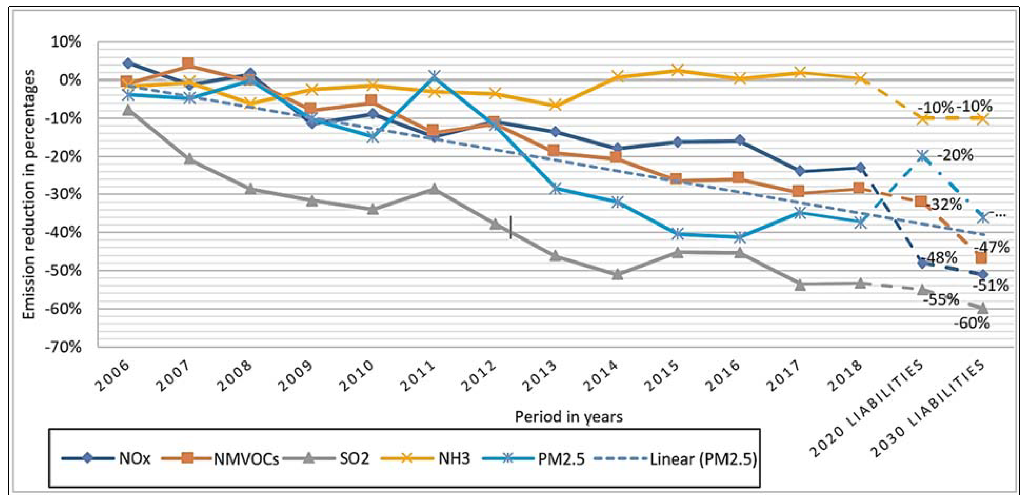
Figure 1. Reduction (%) of the main pollutants’ NOx–nitrogen oxides, NMVOCs–non-methane volatile organic compounds, SO2–sulphur dioxide, NH3–ammonia, PM2.5–particulate matter (2.5 µm a diameter), and Linear (PM2.5)–linear trend for particulate matter (2.5 µm a diameter) in ambient air compared to 2005 and emission reduction commitments by 2020 and 2030.
Sustainability 14 02470 g001
Figure 2. PM10 air pollution measured in the Vilnius agglomeration by 4 municipal air pollution monitoring stations located in Žirmūnai, Savanorių Avenue, Lazdynai and Vilnius Old Town from 2018 to 2020: (a) particulate matter (PM10, µg/m3) average of concentration by annual recorded amounts; (b) number of days when the recorded daily limit value for PM10 (50 µg/m3) was exceeded in the period of 2018–2020.
Sustainability 14 02470 g002
Figure 3. CO and NO2 air pollution measured in the Vilnius agglomeration by 4 municipal air pollution monitoring stations located in Žirmūnai, Savanorių Avenue, Lazdynai and Vilnius Old Town in the period of 2018–2020: (a) carbon monoxide (CO) maximum concentration in a period of 8 h was calculated by means of a moving average; (b) average annual concentration of nitrogen dioxide (NO2).
Sustainability 14 02470 g003
Figure 4. SO2 air pollution measured in the Vilnius agglomeration by 3 municipal air pollution monitoring stations located at Savanorių Avenue, Lazdynai and Vilnius Old Town from 2018 to 2020: (a) maximum concentration of sulphur dioxide (SO2) per 1 h in the period of 2018–2020; (b) maximum daily concentration of sulphur dioxide (SO2) in the period of 2018–2020.
Sustainability 14 02470 g004
Figure 5. Estimated marginal means of CO pollution in the Vilnius Old Town, the values recorded in the 7–31 July 2019 and in the 7–31 July 2020.
Sustainability 14 02470 g005
Figure 6. Estimated marginal means of pollutants in the Vilnius Old Town, between values recorded in the 7–31 July 2019 and 7–31 July 2020: (a) PM10; (b) NO2; (c) SO2_1 h; (d) SO2_24 h.
Sustainability 14 02470 g006aSustainability 14 02470 g006b
Figure 7. MLPN1 (4-4-2) model’s predicted pseudo-probability is presented in a box-plot diagram for the two SIT variable groups.
Sustainability 14 02470 g007
Figure 8. Graphical validation of the MLPN1 (4-4-2) model using the ROC curve.
Sustainability 14 02470 g008
Figure 9. Model performance measurement: (a) cumulative gains that illustrate the accurate classifications gained by the MLPN1 model; and (b) lift chart shows the MLPN1 model performance in a portion of the statistical sample.
Sustainability 14 02470 g009
Table 1. Characteristics, causes and effects by the type of air pollution.
Air Pollution CharacteristicsPollutantsInfluence
Photochemical smog Tailpipe emissions from automobiles. Ozone (O3), by reaction between Volatile Organic Compounds (VOCs), and Nitrogen Oxides (NOx) and water in the presence of sunlight. Health, vegetation and material damages.
Acid RainSulphur Dioxide (SO2) and Nitrogen Dioxide (NO2) react with H2O to form sulphuric and nitric acid.Health, vegetation and material damages.
Stratospheric ozoneChlorofluorocarbons (CFCs)More intense ultraviolet radiation towards the earth.
Greenhouse EffectMan-made pollutants including Carbon Dioxide (CO2), Methane (CH4), Nitrous Oxide (N2O), O3, and CFCsRaising the average temperature on Earth, resulting in slight melting of polar ice-caps and a consequent rise in the sea level.
Source: Levinson et al. [39].
Table 2. Vehicle Pollution Emissions.
PollutantDescriptionImpact
Carbon dioxide (CO2)A by-product of combustion.Fuel production and engines.
Carbon monoxide (CO)A toxic gas which undermines blood’s ability to carry oxygen.Fuel production and engines.
CFCsDurable chemical harmful to the ozone layer and climate.Older air conditioners, aerosol.
Fine particulates (PM10; PM2.5)Inhalable particles consisting of bits of fuel and carbon. Diesel engines and other sources.
Hydrocarbons (HC)Unburned fuel. Forms ozone.Fuel production and engines.
LeadElement used in older fuel additives. Fuel additives and batteries.
Methane (CH4)A gas with significant greenhouse gas properties.Fuel production and engines.
Nitrogen oxides (NOx)Various compounds.Some are toxic, and all contribute to ozone.
Ozone (O3)Major urban air pollution problem resulting from NOx and VOCs combined in sunlight.NOx and VOC.
Road dustDust particles created by vehicle movement.Vehicle use.
Sulphur Oxide (SOx)Lung irritant, causes acid rain.Diesel engines.
Volatile organic hydrocarbons (VOCs).A variety of organic compounds that form aerosols.Fuel production and engines.
Toxics (e.g., benzene)VOCs that are toxic and carcinogenic.Fuel production and engines.
Sources: US EPA (1999a) [14]; ORNL (2000), [31].
Table 3. Mean performance statistics of air pollution in the Vilnius Old Town.
Pollutant7–31 July 20197–31 July 2020Paired Mean
Differences
Cohen’s d
(Rating)
MeanStd.
Deviation
MeanStd.
Deviation
PM10 (g/m3)21.4006.51318.0404.1183.36 *0.434 (small)
3 CO (mg/m3)0.2760.0720.3640.064−0.09 **0.806 (large)
1 SO2_1 h (g/m3)4.5120.1762.6840.4151.83 **3.665 (large)
2 SO2_24 h (g/m3)5.2120.1883.9720.9121.24 **1.391 (large)
NO2 (g/m3)35.48016.07830.3009.0865.180.287 (small)
Notes: 1 SO2_1 h–SO2 maximum concentration per one hour; 2 SO2_24 h–SO2 maximum daily concentration. 3 CO maximum concentration per 8 h; Significant difference: * p < 0.05, ** p < 0.01.
Table 4. MLP network description for data processing.
LayerPartitionsNumber of UnitsActivation Function1 Variable Description
MLPN1:4-4-2
Input28.0%5-IV: PM10, CO, SO2_1 h, SO2_24 h, NO2
Hidden (1)40.0%10Hyperbolic tangent
Hidden (2)5
Output30.0%2IdentityDV: (SIT: 1 = July 2019; 2 = July 2020)
MLPN2: 5-3-2
Input44.0%5-IV: PM10, CO, SO2_1h, SO2_24 h, NO2
Hidden (1)34.0%10Hyperbolic tangent
Hidden (2) 5
Output22.0%2IdentityDV: (SIT: 1 = July 2019; 2 = July 2020)
MLPN3: 6-2-2
Input60.0%5-IV: PM10, CO, SO2_1 h, SO2_24 h, NO2
Hidden (1)20.0%10Hyperbolic tangent
Hidden (2) 5
Output20.0%2IdentityDV: (SIT: 1 = July 2019; 2 = July 2020)
1 Notes: IV = independent variable; DV = dependent variable; PM10–average daily concentration; CO–maximum concentration per one hour; SO2_1 h–SO2 maximum concentration per one hour; SO2_24 h–SO2 maximum daily concentration; NO2–maximum concentration per one hour. Standardized rescaling method for covariates; Error Function = Sum of Squares.
Table 5. Summary for the designed models.
Layer DescriptionMLPN1
4-4-2
MLPN2
5-3-2
MLPN3
6-2-2
1 TrainingSum of Squares Error0.0050.0080.411
Percent Incorrect Predictions0.0%0.0%0.0%
Training Time0:00:00.010:00:00.010:00:00.01
TestingSum of Squares Error0.0210.0570.075
Percent Incorrect Predictions0.0%0.0%0.0%
HoldoutPercent Incorrect Predictions0.0%33.3%0.0%
1 Notes: Dependent variable: SIT: 1 = July 2019; 2 = July 2020. Stopping rule used = consecutive step(s) with no decrease in error.
Table 6. Model sample classification using the constructed MLPNs.
SampleObserved1 Predicted Dependent Variable
MLPN1 (4-4-2)MLPN2 (5-3-2)MLPN3 (6-2-2)
SIT1SIT2Percent CorrectSIT1SIT2Percent CorrectSIT1SIT2Percent Correct
TrainingJuly 2019100100.0%100100.0%150100.0%
July 2020010100.0%013100.0%015100.0%
Overall Percent50.0%50.0%100.0%43.5%56.5%100.0%50.0%50.0%100.0%
TestingJuly 2019100100.0%130100.0%50100.0%
July 2020010100.0%05100.0%05100.0%
Overall Percent50.0%50.0%100.0%72.2%27.8%100.0%50.0%50.0%100.0%
HoldoutJuly 201950100.0%20100.0%50100.0%
July 202005100.0%3457.1%05100.0%
Overall Percent50.0%50.0%100.0%55.6%44.4%66.7%50.0%50.0%100.0%
1 Notes: Dependent variable = SIT: SIT1 = July 2019, SIT2 = July 2020.
Table 7. The area under the curve.
MLPN1
40%-40%-20%
MLPN2
50%-30%-20%
MLPN3
60%-20%-20%
AreaAreaArea
1 SITSIT1 = July 20190.9981.0001.000
SIT2 = July 20201.0001.0001.000
1 Notes: Dependent variable = SIT: SIT1 = July 2019, SIT2 = July 2020.
Table 8. Importance of independent variables for air quality prediction.
1 VariablesMLPN1
40%-40%-20%
MLPN2
50%-30%-20%
MLPN3
60%-20%-20%
ImportanceNormalized
Importance
ImportanceNormalized
Importance
ImportanceNormalized
Importance
PM100.15439.4%0.0335.9%0.11621.8%
CO0.23059.0%0.25946.6%0.18033.8%
SO2_1 h0.390100.0%0.557100.0%0.533100.0%
SO2_24 h0.13234.0%0.11821.1%0.13926.1%
NO20.09424.2%0.0346.0%0.0315.8%
1 Notes: PM10–average daily concentration; CO–maximum concentration per one hour; SO2_1 h–SO2 maximum concentration per one hour; SO2_24 h–SO2 maximum daily concentration; NO2–maximum concentration per one hour.
Publisher’s Note: MDPI stays neutral with regard to jurisdictional claims in published maps and institutional affiliations.