Economic Assessment of Urban Ash Tree Management Options in New Jersey

Abstract

A cost–benefit analysis (CBA) is an economic approach to estimate the value of alternative programs, policies or management options. Net present value in CBA is one of the standard approaches to value the future benefits of investments. Due to the complexity of urban tree benefits, little is known about how to estimate the monetary value of the ecosystem services that urban trees provide as future benefits. We modeled the economic analyses of emerald ash borer (EAB) (Agrilus planipennis) management scenarios for urban ash trees (Fraxinus spp.) in New Jersey. These scenarios include: (1) no infestation or baseline scenario, (2) infestation with no action, (3) immediate removal and replacement and (4) the treatment of ash trees. The net present value for each management option is calculated using discount rates of 0%, 2% and 5%. The National Tree Benefit Calculator (NTBC) tool is used to quantify the economic value of the ecosystem services provided by the ash trees based on their diameter at breast height (DBH) values. The horizon over which benefits and costs are calculated was set at up to 20 years to estimate the net present value of ash trees that have DBH values of 4 inches. Results from the NPV outputs conclude that across most discount rates, the treatment of ash trees provided greater dollar (USD) values of ecosystem services over time when compared to inaction or the removal and replacement of ash trees. The present research suggests that removing and replacing ash trees is not cost effective at any discount rate due to the high future costs associated with retaining the newly planted trees over a twenty-year time horizon.

1. Introduction

The emerald ash borer (EAB) (Agrilus planipennis) is a wood-boring beetle present in the U.S. that is native to Asian countries, including China, Japan, Taiwan, Korea, Laos, Mongolia and the Russian Far East [1,2,3,4,5,6]. It most likely entered the U.S. in solid wood packing material, pallets, crates or containers from international commerce related to shipments from Asia [7,8]. EAB attacks all members of the genus Fraxinus in the continental U.S. [5,9,10,11] and southern Canada [12]. EABs have killed billions of ash trees across the U.S. and Canada since 2002 [13,14]. The EAB was first identified in the U.S. near Detroit in southeastern Michigan in 2002. Since its initial dispersal in Michigan, the EAB has killed over an estimated 8 billion of native ash trees (Fraxinus spp.) and is currently dispersed across both the U.S. and Canada [15,16,17]. Due to biological flight and anthropogenically driven flight dispersal modes, the EAB infestation continues to broadly spread across the Midwestern and Northeastern states in the U.S. [18].

Mature larvae of EABs bore into the outer sapwood, developing serpentine feeding galleries in the cambial and phloem tissue of ash trees, causing rapid tree mortality due to the disruption of sap transportation between shoots and roots [5,19]. As EABs disrupt sap flow, tree water usage decreases by 80%, resulting in reduced leaf area and leaf mass [5]. Reduced photosynthetic rates and internal CO₂ concentrations due to altered foliage contributes to the reduction of nonstructural carbohydrate accumulation in leaf tissue, further damaging phloem and xylem tissue.

In general, Fraxinus pennsylvanica and Fraxinus americana represent a substantial component of municipal tree inventories in the United States, and represent the two most commonly established species within New Jersey, which is the focus of this study [20]. Once infested, EABs can kill a healthy tree within four to seven years of its initial infestation [15,21,22]. EABs can go unnoticed through the earlier stages of infestation, but the infested ash trees die very quickly once larval populations reach critical levels. In terms of its natural flight dispersal, EAB infestations move about 1–10 miles per year [23,24]. Human assisted dispersal modes, such as EABs traveling through “hitchhiking” on vehicles along transportation routes, through nurseries and through the movement of wood through campgrounds, can lead to EAB dispersal across farther areas and increase the rate of EAB dispersal and spread [25].

From the pattern of the North American infestation thus far, nearly all ash trees within the developed landscape will become infested and prematurely die if left untreated. Municipalities and homeowners will likely bear 80% of the cost incurred by EABs [26]. Given the likely widespread EAB invasion in New Jersey, the early evaluation of EAB impact has been crucial for the preservation of and estimating the risk to ash trees across the wildland–urban interface, which can be seen in proximity in New Jersey. Gaining an understanding of EAB management and the insect invasion’s impact on tree loss will better inform our understanding of novel diseases and pest responses in the future. Developing a cogent frame for an economic analysis is desired to help inform the next introduced pest outbreak in a time of forest stress and transition from climate change, and human development pressures in this densely populated, urbanized state within the northeast megalopolis.

Federal, state and local agencies have taken measures to detect, control and prevent the human-assisted spread of the EAB. However, agencies must budget scarce discretionary resources, which makes it difficult to allocate limited funds to alternative methods of prevention and control. The allocation of funding is conditional upon whether the calculable/demonstrable benefits of a suggested management option, such as chemical treatment, outweigh the cost. Due to the urgency of the EAB threat, immediate management action has been required to mitigate the risk, and the tree value is significant factor for the decision to invest in tree management rather than removal.

Forest economic or market value is mostly defined in terms of specific physical products, such as timber, which can be bought and sold at market price. Urban trees are either planted or managed to provide benefits beyond trees’ physical “values” [27]. The non-physical benefits of trees, including environmental, aesthetic and socio-economic values, are arguably intangible and hard to quantify. Therefore, alternative valuation methods need to be used to establish the value of trees as a fundamental baseline to arboriculture and urban forestry [28,29,30,31]. In general, the monetary non-use value of a tree has been based on cultural perceptions of their amenities [32].

Different approaches in the literature have been discussed to determine the value of urban tree benefits [33]. Tree care professionals in New Jersey have typically relied upon tree value appraisal formulae and methods detailed by the Council of Tree and Landscape Appraisers (CTLA) [34], typically including the basic price/in² of a tree, the tree condition and the location of the tree, on a per species basis. Nowak and Greenfield [35] estimated that there were 5.5 billion trees (39.4% tree cover) in urban areas in the U.S. According to their report, these trees annually generate a total of USD 18.3 billion in value, including air pollution removal (USD 5.4 billion), reduced building energy use (USD 5.4 billion), carbon sequestration (USD 4.8 billion) and avoided pollutant emissions (USD 2.7 billion).

An alternative market-based approach includes the market value of property due to tree/trees, such as hedonic pricing methods. Hedonic pricing is used to calculate the housing prices due to the nearby forest or greenspace [36]. The present study deploys the shift from the appraisal value of urban trees favored by the tree care community to an established environmental service value that extend the work of urban tree benefits across the biophysical, economic and social disciplines [37,38,39,40]. Urban forest attributes, such as canopy cover, species, proximity and tree size, have been associated with increased ecosystem service value [41]. Most of the ecosystem service value estimates are based on a national level, but it important to provide refined estimates of ecosystem services and values on a per unit tree basis to develop more localized estimates [35].

Peoples’ willingness to pay to preserve forests is captured in contingent valuation methods [42,43]. The travel cost method is used to proxy the price that people are willing to pay for the recreational benefits of forests [44,45]. These approaches often lack the time horizon, such as net present value over the years, to account for the intangible benefits of trees in terms of explicit cash flows, and lack the capability to isolate the benefits of individual trees within forest stands. We adopted a longer time horizon based on an established treatment timeline of 20 years [46]. The discounted cash flow (DCF) analysis method of valuation is generally lacking in the arboriculture and urban forestry economic discussion. Urban trees are generally assessed by methods of valuation that ignore the time value of money and discounted intangible tree benefits. Estimating future streams of tree benefits has been limited due to a general lack of data on species specific and/or regional growth rates specific to urban trees in contexts with common landscape site parameters. Tree benefits are thus modeled and described in general terms, and the determination of the value of their ecosystem services becomes difficult to measure with any precision or confidence [30]. We have generalized the models of i-Tree, local data and cost–benefit analysis to introduce a DCF component to the analysis which allows for the longer time horizon.

It is difficult for arborists, urban foresters, planners or stakeholders to develop reasonable estimates and projections of tree benefits without a strong financial background and familiarity with complicated software and statistical methods. In addition, how to use those benefits to make a decision to select a cost-effective EAB management option is another challenge. To meet this challenge, a similar tool was developed by Sadof et al. [47] to provide policy makers with a web-based EAB management cost calculator to compare the discounted annual and cumulative costs of EAB management strategies. Their research suggested that strategies based on saving ash trees were cost effective and ecologically beneficial compared to those strategies that mostly removed and replaced ash trees.

Among others, the recently developed National Tree Benefits Calculator (NTBC) provides the tree benefits in terms of ecosystem services, such as storm water management, air quality, property value, carbon sequestration and energy savings [27]. The data system chosen for this analysis uses the NTBC. The NTBC database of urban tree benefit information is an open-access resource that can be accessed by anyone online [48]. The NTBC allows users to estimate the ecosystem service value with the use of a common measure, diameter at breast height (DBH), which is trunk diameter at 4.5 ft above ground level. DBH and location-specific structures provide a very specific ecosystem benefits calculation within the NTBC and the i-Tree service modeling frames. DBH is commonly used by arborists and forestry professionals, and can be implemented in net benefit calculations, since DBH-based growth rate data across many regions and species are readily available.

NTBC facilitates the calculation of the benefit function, but lacks cost data for management needs. In this regard, this paper will situate itself in the larger body of work, such as that on Milwaukee, WI and other cities, that focuses on managing the emerald ash borer (EAB) through active urban forest management with a complete understanding of risks and value [47,49]. We proposed that there is a fixed set of data streams which can be rapidly and simplistically developed and deployed with the NTBC to help these audiences in an organized way. This will help in evaluating a set of management strategies for any manner of diseases or pest outbreaks.

Incorporating discounted tree valuation in management options can inform decision making in response to pest infestation and uncertainty. We propose a discounted cost benefit valuation method using NTBC, facilitating the evaluation of management options for foresters. This study focuses on the economics of management practices that will enable effective decision-making capabilities to manage urban trees, and management options for sustainable and economically viable forestry practices. The development of a discounted valuation model is built on cost–benefit analysis to bridge the gap between forest management and economic decision making. It allows incorporating ash tree data with DBH, and incorporating these data with the NTBC and forest management practices within a unified framework.

The present study aims to facilitate the economically enhanced management of ecological resources, with a focus on both economic viability and adaptation to the changing climate. Making decisions that have high ecological and economic impact will require new ways of addressing the challenges of robustness and interpretability.

In this regard, this paper presents a method to demonstrate the implementation of discounted tree valuation using the NTBC to evaluate the EAB management decisions, including no action, the removal and replacement of ash trees and the treatment of ash trees in a benefit–cost scenario. The primary goal of this modeling exercise is to provide policy makers with the quantitative guidance for cost-effective alternative strategies to control, prevent or slow the spread of EAB, and to account for the time value of benefits in each management decision. Secondarily, since we know that exotic pest introduction, damage and management in community forests are likely to happen again, this process seeks to frame a debate and an approach to help guide future pest responses.

We implemented geospatial data, urban forest management options, economic cost–benefit analysis and the ecosystem service valuation of ash trees. The major objectives of this paper include:

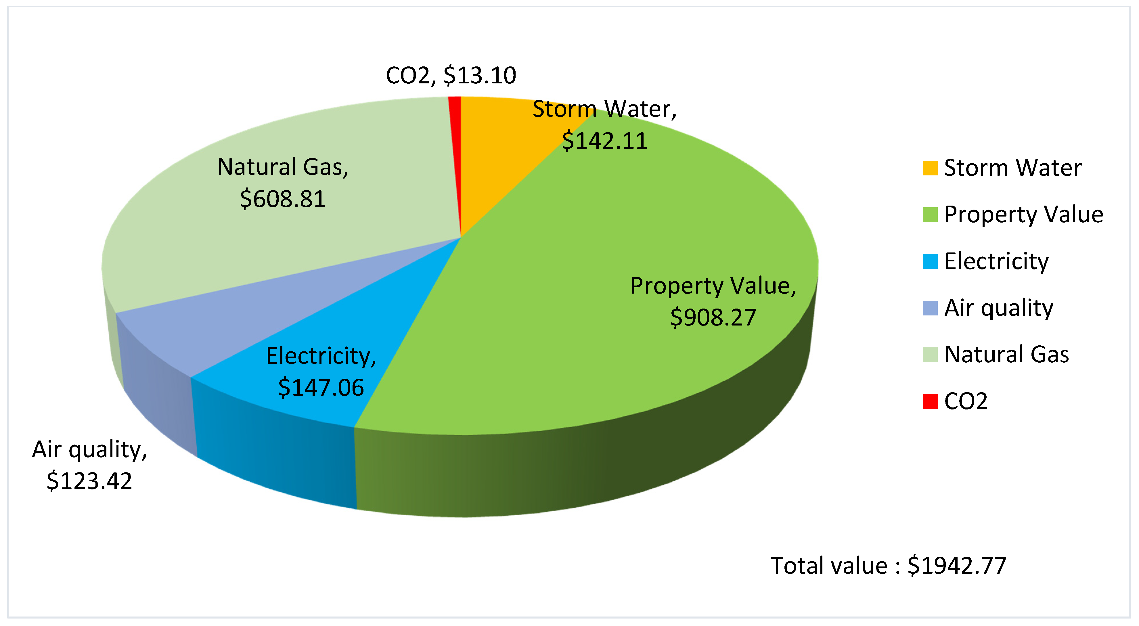
• To quantify the economic value of ecosystem services, including storm water, property value, energy, CO₂ and air quality by ash tree.
• To conduct a net present value analysis of future benefits and costs for each of the four EAB management scenarios.

2. Material and Methods

2.1. Case Study

In New Jersey, 9% of the state’s total forested area consists of 24.7 million ash trees [50]. These ash trees are vulnerable to an EAB infestation. The majority of the ash trees in New Jersey are in the north-western part of the state [17]. Additionally, ash has been traditionally planted as a popular and inexpensive street and landscape tree species. Infested trees on public and private properties in urban areas pose a hazard due to the risk of falling branches that have the potential to hit people and damage property or infrastructure.

The EAB was first detected in Bridgewater, Somerset County, New Jersey, in May 2014. By 9 December 2019, the Emerald Ash Borer has been found in New Jersey in 15 counties across 70% of the state [17]. As the EAB continues to spread and intensify throughout New Jersey, it is accompanied by substantial economic impacts associated with the loss of trees. The management choices have profound impacts on the urban and rural canopy and the accompanied consequences on the ecosystem services they provide. Across the U.S., the EAB is causing billions of dollars (USD) in costs for tree removals, replacement, and insecticide treatments [17,51,52].

To develop a statewide understanding of the EAB management issue, we chose an existing genus-level roadside survey which counted ash trees by occurrence and DBH across forty-three municipalities and 12 counties in New Jersey [53].

The Rapid Ash Survey provided a proximate location for municipal ash tree DBH distribution with a population demographic of 5406 geo-located road-side ash trees. The DBH for the Rapid Ash Survey ranged from 1 to 70 inches. The highest number of ash trees from the 2015 rapid assessment were found in Burlington County.

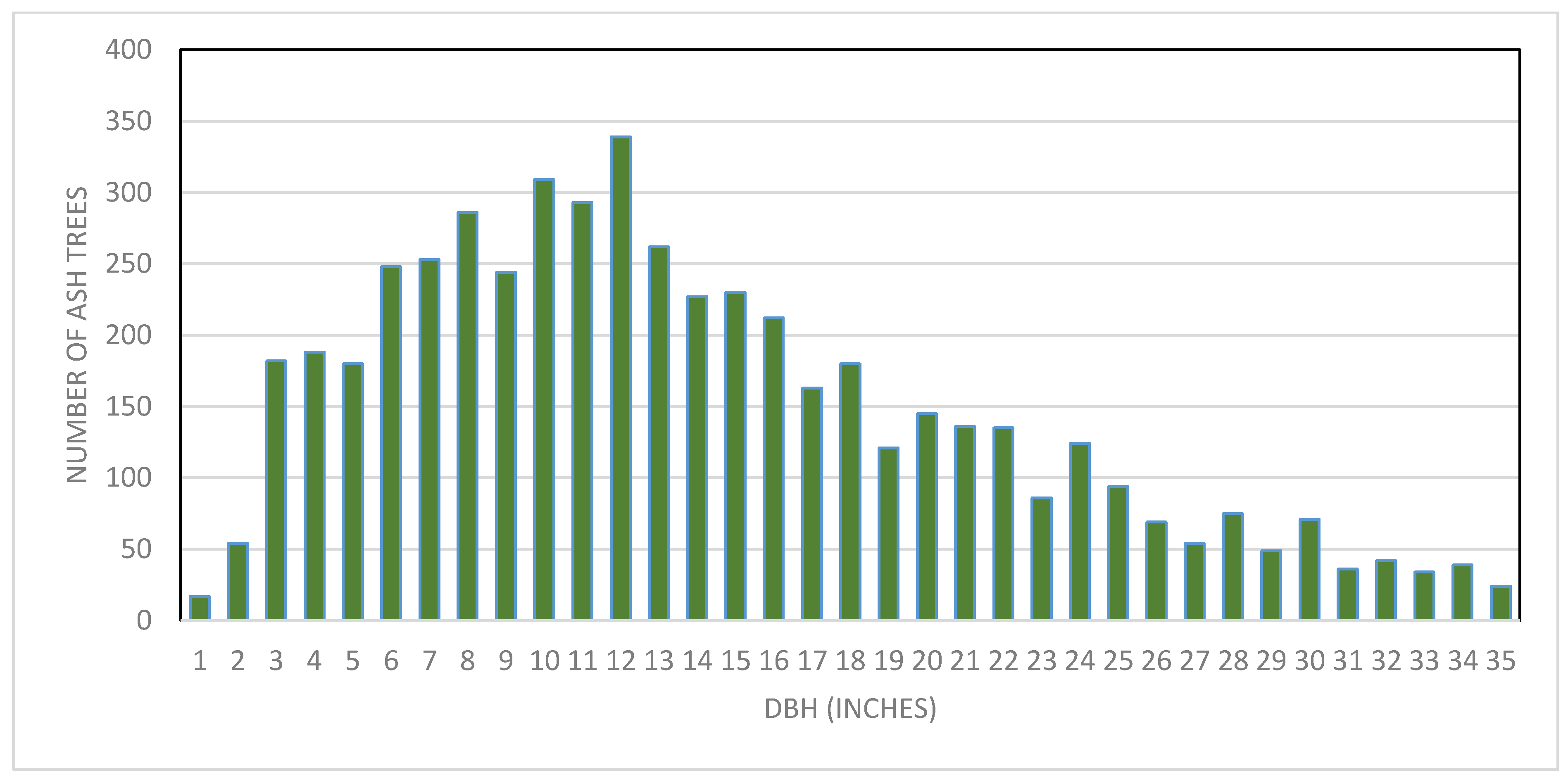
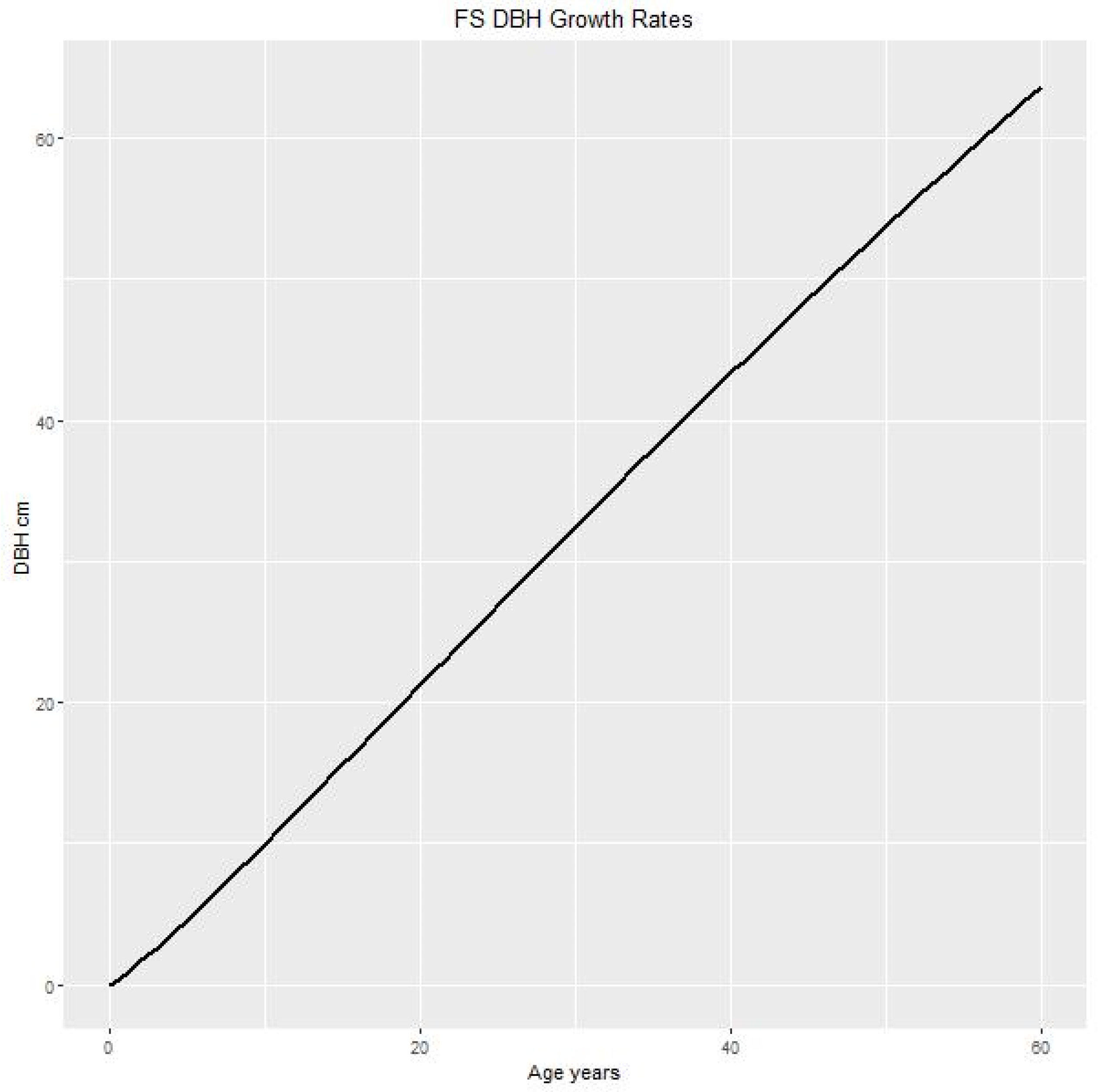
2.2. Ash Tree Age, DBH and Growth Rate

In the model analysis, the benefits conveyed by ash trees are directly related to DBH in the NTBC model structure. The Tree Benefit Calculator provided easy-to-estimate annual benefits of street-side trees. The NTBC is based on the i-Tree assessment tool, called i-Tree Streets [48]. It allows anyone to obtain economic and environmental benefits in terms of dollar (USD) value on an annual basis using location, species, and tree size [48].

DBH can be converted into an age in years using existing generalized tree growth curves. In our case, a dataset of 264 urban ash trees within north and central New Jersey were measured for DBH, and the increment profiles were collected using a resistance drill calibrated to the genus with 20 physical cores to determine tree annual ring counts. These data were further used to generate specific DBH to age curves (unpublished data).

A Chapman–Richards growth model was used to assess the relationship between age and DBH (cm). Age, in years, was used as the independent variable, and cumulative basal area (BA), in cm², was used as the dependent variable. Although a sigmoidal curve would typically be expected, no tree measured was at an age where the sigmoidal features would be evident. The Chapman–Richards growth function was used to model this relationship due to its superior performance over other similar models, such as the Richards, von Bertalanffy and Weibull models [54,55,56,57].

The Chapman–Richards growth equation is:

$$y={\beta }_0{\left[1-\exp \left(-{\beta }_{1}x\right)\right]}^{\frac{1}{1-{\beta }_2}}$$

(1)

In this model, y represents the cumulative basal area at age x, ${\beta }_0$ is the asymptote, ${\beta }_1$ is the growth rate and ${\beta }_2$ is a shape parameter. All parameters, except for ${\beta }_0$, were estimated. Parameter values for ${\beta }_0$ were established by using data from the NJ Forest Service 2020 “Big Trees” registry. The model was constructed and run using OpenBUGS [58] software, which uses Gibbs sampling.

To link the NTBC benefits to age through a shared DBH relationship, we used correlation plots between annual growth rate and age, and DBH and annual growth rate. An ash tree average annual growth rate of 0.46% per inch based on the 264 urban ash trees increment profiles was used. The time horizon for discounted benefits was determined based on the DBH value suggested in Lovallo and Grabosky’s study [59], with an average growth rate factor of 0.46%.

We deployed the linear DBH and average annual growth rate relationship to calculate the total benefit function for the ash trees in New Jersey based upon the NTBC structured in the following linear form:

$$\mathrm{Vn}\left(\mathrm{DBH}\right)=\mathrm{SW}+\mathrm{PV}+\mathrm{E}+\mathrm{AQ}+{\mathrm{CO}}_2$$

(2)

where $\mathrm{Vn}$ is the total annual benefit in dollars (USD) of a given tree based on DBH. DBH is defined as a function of the growth rate in the model. SW, PV, E, AQ and CO₂ are ecosystem service benefits from storm water, property value, energy, air quality and carbon sequestration, respectively (

Table 1. Environmental and Economic Benefits. Adapted from [48].

Benefits	Details as Described in the NTBC, 2021
Storm Water	Trees reduce urban storm water runoff (or “non-point source pollution”) by: Intercepting and holding rain on leaves, branches and bark. Increasing the infiltration and storage of rainwater through the tree’s root system. Reducing soil erosion by slowing rainfall before it strikes the soil.
Property Value	The NTBC uses a tree’s Leaf Surface Area (LSA) to determine increases in property values. A home with more trees (and a higher LSA) tends to have a higher value than one with fewer trees (and a lower LSA).
Energy	Trees reduce kilowatt hours of electricity for cooling and reduce the consumption of oil or natural gas. Trees modify the climate and conserve building energy use in three principal ways: Shading reduces the amount of heat absorbed and stored by buildings. Evapotranspiration converts liquid water to water vapor and cools the air by using solar energy that would otherwise result in the heating of the air. Tree canopies slow down winds, thereby reducing the amount of heat lost from a home, especially where conductivity is high (e.g., glass windows).
Air Quality	Urban forests can mitigate the health effects of pollution by: Absorbing pollutants, such as ozone, nitrogen dioxide and sulfur dioxide, through leaves. Intercepting particulate matter, such as dust, ash and smoke. Releasing oxygen through photosynthesis. Lowering air temperatures, which reduces the production of ozone. Reducing energy use and subsequent pollutant emissions from power plants.
CO2	Trees can have an impact by reducing atmospheric carbon in two primary ways: They sequester (“lock up”) CO2 in their roots, trunks, stems and leaves while they grow, and in wood products after they are harvested. Trees near buildings can reduce heating and air conditioning demands, thereby reducing emissions associated with power production.

).

Local managers might consider direct measures from stumpage or sample cross-sections at DBH from a limited number of trees removed in the management zone using similar method within popular computer spreadsheets programs. It could be refined to identify relationships over subsequent observations, or used until a more formal research treatment becomes available for the species and regions in play.

2.3. Costs

Removal costs as a function of DBH are estimated by using a survey of New Jersey tree care professionals [53]. Local managers may use specific estimates from professional tree care contractors that work with the municipality.

2.4. Ecological Benefits of Urban Ash Trees

The dollar (USD) value of ecological benefits is extracted from the National Tree Benefit Calculator [48] and further linked to a net present value (NPV) model. NPV computes the discounted monetary value of a single tree over a time horizon. From this model structure, we tested a series of four management scenarios, including no infestation, infestation with no action, immediate removal and replacement, and insecticide treatment on three discount rates of 0%, 2% and 5% to appraise the value of differing management approach decisions on our test population. Different discount rates provide the scenario analysis with varying future value. Monetized ecosystem benefits, including storm water, property value, energy, air quality and carbon sequestration, were developed from the NTBC by implementing the information on DBH ranges found in the Rapid Ash Survey, and growth rate data from 264 ash tree profiles.

For each input of location and DBH of ash trees, the NTBC returns benefit values for each “environmental service” category per year accounting for growth by DBH as related to other tree dimensions. Quantitatively, the general model can be viewed as a sum of benefits calculated on an annual basis in the summation form:

$$NP{V}_{\mathrm{V}}={\displaystyle \sum }_{i=1}^k{\beta }_{\mathrm{vn}}+{\beta }_{\mathrm{vn}+1}+\dots {\beta }_{\mathrm{vk}}$$

(3)

where NPVv is the net present value of the discounted benefits v, and v is based on DBH: $V=f\left(DBH, r\right)$, where r is average annual growth rate.

V_n in Equation (3) represents the discounted summation of each benefit for the first year (n increases each year by factor i). V_k represents the discounted benefits from the final year. NPV estimates (the present value of tree benefits minus the present value of tree costs) can be regarded as a yield on the ash tree investment across various management scenarios.

2.5. Analysis of Management Scenarios

The timeline of events in EAB management plans was set to 20 years. Therefore, the horizon over which benefits and costs are calculated was up to 20 years. This time horizon leaves the analysis greater than the maximum observed DBH in the field. Additionally, this time horizon is chosen in consideration of the expectation of the infestation treatment period and the return interval.

Morin et al. [22], in their proceedings paper and subsequent work in an updated and expanded form, found that ash mortality was initially very low, and was between 1 and 2% per year in the years after EAB detection. Ash mortality due to EABs increased slowly over time, and the authors found only 3–4% per year for 7–8 years post detection. These results are consistent with the dendrochronological analysis of the history of ash mortality in southwest Michigan by Seigert et al. [14]. They concluded that ash trees were dying there as early as 1997, and that the EAB was present since at least the early to mid-1990s. Klooster et al. [60] found that ash mortality did not reach 40% in the southeast Michigan until 2005, but then accelerated quickly to 99% by 2009. Burr and McCullough [61] provided data from 2011 on the percentage of ash mortality at sites throughout southern Michigan at varying distances from the epicenter of the invasion, including 87% near the core, where the EAB had been first detected nine years previously.

Knight et al. [21] found that the first infestation occurred two years prior to the first detection of an exit hole at breast height. However, studies have shown that EAB first colonizes the upper canopy, and that trees are generally in severe decline by the time exit holes appear at breast height [62]. The Knight et al. [21] study sites were clearly infested for a much longer time than their model assumption.

Because the EAB is notoriously hard to detect when populations are low, the year of first infestation is not a useful parameter on which to base the tree mortality in the model, as it is impossible to determine in practice. Following the method of Morin et al. [63], the year of first detection is an operationally feasible parameter, but it is not clear how the year of detection relates to the year of establishment, as some populations were well established, with tree mortality underway before they were detected, while other infestations were detected based on trap captures, when EAB densities were still too low to cause tree mortality.

In this model, based upon the assumptions set in Knight et al., [21], and Morin et al., [22], the ash tree mortality rate was captured in three different years after initial EAB infestation. These studies also show that tree level factors, such as DBH and age, are crucial in predicting the survival rate of ash trees. The mortality rate chosen in this paper has been established at local as well as regional scales [10,21,22,64]. The assumption that it will take 10, 15 and 20 years from the onset of EAB infestation until all untreated trees are lost is set as a functional prediction. Therefore, the EAB mortality occurs in year 10, 15 and 20 in the model, and trees are removed and replaced in these years.

2.5.1. No Infestation

As a baseline from which to compare the other scenarios, we assume there is no EAB infestation, and the present value of the stream of benefits over a 20-year horizon for the existing ash tree with initial DBH is:

$$P{V}_{NI}={\displaystyle \sum }_{n=0}^{20}\frac{V_n}{{\left(1+i\right)}^n}$$

(4)

where V_n is the benefit of the ash tree obtained at year n, and i is the discount rate (expressed as a decimal). Due to the absence of cost, this management scenario tends to have the highest overall present value in comparison to other scenarios.

The change in net loss value to the homeowner or municipality in the no infestation scenario is zero.

2.5.2. Infestation and No Action

As the EAB begins to infest the ash trees, many of the infested trees will begin to die. These trees will often become a safety hazard, and their removal will be necessary. This option entails only acting upon the dead trees that are actively dangerous to the population. The removed trees are not replaced with the new ones. Due to the trends of the damage caused by EABs, however, many of these trees will die in a very short period, causing an influx of unsafe ash trees that must be removed in the short span of a few years. Typically, most of the trees will need to be removed within 10, 15 and 20 years after the introduction of the emerald ash borer. In this scenario, we assume that an infestation occurs in year zero and proceeds to kill each ash tree within 10, 15 and 20 years. This means that ash trees become infested as a function of insect population growth. The present value of this scenario discounted at 10, 15 and 20 years includes the benefits of the existing ash tree and the removal cost:

$$P{V}_{NA}={\displaystyle \sum }_{n=0}^n\frac{V_{NA}-C_R}{{\left(1+i\right)}^n}$$

(5)

where V_NA is the benefit of the ash tree obtained at year n, C_R is the cost of removing the dead ash tree at year n and n is 10, 15 and 20 years from the initial infestation.

The change in net loss value to the homeowner or municipality in the infestation and no action scenario is in each mortality year (n) is:

$$\Delta N{V}_{NA}=P{V}_{NA}-P{V}_{NI}$$

(6)

where $\Delta N{V}_{NA}$ represents the change in net loss value to the homeowner or municipality with an EAB infestation in year n when no action is taken. The present value of this scenario is subtracted from the present value of no infestation (Equation (4)) to calculate the net loss value.

2.5.3. Immediate Removal and Replacement

In this scenario, an infested ash tree is immediately removed and replaced with a non-host species. The present value of this scenario includes the cost of the removal and replacement and the benefits of the replacement tree over the 20-year time horizon:

$$P{V}_{RR}={\displaystyle \sum }_{n=0}^{20}\frac{V_n-C_{RR}}{{\left(1+i\right)}^n}$$

(7)

where C_RR is the cost of removing and replacing the existing ash tree and V_n is the benefit of the replacement tree in year n. The cost of the replacement tree is the sum of the cost of removal, and cost of the replacement of a new tree. The model, as used in this study, assumes that replacement trees have the same annual benefit over 20 years as ash trees. It is also assumed, in the model, that all replacement trees species with similar biological growth characteristics will start with the 4-inch DBH, as suggested in Lovallo and Grabosky (2015) [59]. No pesticides or other treatments are utilized in this scenario. The NPV of a single tree is aggregated to a community population. This plan discards many healthy trees that provide real economic value to the city. This is a potentially costly option.

The change in net loss value to the homeowner in the immediate removal and replacement scenario is:

$$\Delta N{V}_{RR}=P{V}_{RR}-P{V}_{NI}$$

(8)

2.5.4. Treatment of Ash Trees

In this scenario, we assume that the ash tree is treated with a systemic insecticide every year, beginning in year zero. As a result of treatment, the tree is protected against infestation, survives and provides benefits over the 20-year horizon. The present value of this scenario is:

$$P{V}_T={\displaystyle \sum }_{n=0}^{20}\frac{V_n-C_T}{{\left(1+i\right)}^n}$$

(9)

where C_T is the cost of insecticide treatment. In this scenario, the evaluation of chemical treatment on tree health was not included due to real data limitations.

The change in net loss value to the municipalities, planners, and homeowners in the treatment of ash trees scenario is:

$$\Delta N{V}_{TT}=P{V}_{TT}-P{V}_{NI}$$

(10)

If an infestation occurs in year zero, then a comparison of present values of scenarios 2, 3 and 4 shows the relative values of no action, immediate removal and replacement, and the treatment of the ash tree respectively. The difference between the present value of the benefits of the ash tree without infestation (scenario 1) and the present value of the benefits associated with any one of the management options (scenarios 2, 3 or 4) represents the change in the net loss/benefits to the municipalities and planners, as well as homeowners. This change in net loss is an estimate of the cost of the EAB infestation.

3. Results

3.1. Ash Tree Age, DBH and Growth Rate

The distribution of ash trees found in the Rapid Ash Survey is shown in Figure 1 and Figure 2. The majority of ash trees were found with around 12 inches of DBH (Figure 1). This DBH was also used as last year’s DBH, informing the model from real data. Most of the ash trees were found in the Ewing township (Figure 2).

Three Markov chains were run simultaneously in the R environment [65]. After 10,000 iterations, the three chains were visually verified to have achieved convergence, and a stationary distribution was reached. The iterations to achieve convergence were considered to be part of the “burn-in” period. The model was run for an additional 50,000 iterations to generate the sample space. The parameters were estimated from the generated sample space based on prior and hyperprior probability distributions.

The estimated parameters are as follows:

$${\beta }_0=33560,{\beta }_1=0.007358 , {\beta }_2=0.5629$$

(11)

Once the parameters for the basal area were estimated, the DBH was calculated via the following model:

Conversion to DBH:

$$y=\sqrt{\frac{4}{\pi }{\beta }_0{\left[1-\exp \left(-{\beta }_{1}x\right)\right]}^{\frac{1}{1-{\beta }_2}}}$$

(12)

A Chapman–Richards growth function between age and DBH (cm) for Fraxinus species shows a positive relatioship (Figure 3).

The benefits of all urban ash trees using the NTBC are found to be uniform across New Jersey due to the uniform climatic zone. The age and growth rate, and DBH and growth rate are well correlated due to the old urban ash trees with a consistent diameter distribution (Figure 4 and Figure 5). These data do not extrapolate beyond the maximum diameters allow to estimate ecosystem services value in NTBC. This provides the basis of the ash tree age from which to investigate the benefits based on the size of the DBH for the NPV calculations.

3.2. Ash Tree Benefits

The total annual benefits calculated from the NTBC ranged from USD 57.29 to USD 137.42 for a DBH range of 4.12 inches to 12.82 DBH trees, respectively, which results in an additive function that can be estimated over time. With a 0.46% annual growth and an initial 4-inch DBH, we found a 12.82-inch DBH for the year 20 (time horizon). Within this selection of DBHs, the tree benefits result shows that, among the total tree benefits, property values were among the most highly observed benefits due to urban ash trees (Figure 6).

3.3. Costs

The values for the cost of tree removal and replacement in this study are based on New Jersey estimates ([59],

Table 2. Costs in the economic model.

Title	Costs (USD )
Average cost of the large (12-inch DBH) ash tree	USD 325
Replacement of ash tree cost	USD 325
Removal cost	USD 45 per inch of DBH
Treatment cost	USD 5 per inch of DBH

). The established NJ statewide average cost for the largest commonly available and transplantable tree is USD 325 [59]. Lovallo and Grabosky, [59], suggested that the removal cost and treatment cost of ash trees are USD 45 per inch and USD 5 per inch DBH, respectively. The cost of treatment assumes a bulk price for emamectin benzoate of 5 USD/inch of DBH [47].

3.4. EAB Management Scenarios

3.4.1. No Infestation (Baseline Scenario)

This scenario has no cost, so we just calculated the NPV. The NPV over a 20-year horizon of a tree starting at 4 inches in year 0 are added up over 20 years, resulting in an increase in present value (

Table 3. NPV at 0%, 2% and 5% discount rates.

Management Scenario	Net Present Value USD (0%)	Net Present Value USD (2%)	Net Present Value USD (5%)
No infestation (over 20 years)	1942.77	1542.79	1126.13
Infestation and no action (over 10, 15, 20-year horizon)	−2023.27, −3648.73, −5682.93	−1793.37, −3047.89, −4470.45	−1511.55, −2371.38, −3215.33
Immediate removal and replacement (over 20 years)	−12,182.93	−9784.67	−7265.55
Treatment (over 20 years)	1095.47	874.65	643.75

). The increase is higher with the lowest discount rate (Table 3). This increase in present value results from a lack of cost of infestation.

3.4.2. Infestation and No Action

Infestation and no action resulted in decreases in the NPV with the increase in the time horizon, and with larger decreases in the NPV at lower discount rates (Table 3). Subsequently, this results in higher loss values for ash trees with the increase in the time horizon and at a 0% discount rate (

Table 4. Net loss value at 0%, 2% and 5% discount rates.

Management Scenario	Net Loss Value USD (0%)	Net Loss Value USD (2%)	Net Loss Value USD (5%)
No infestation (over 20 years)	0	0	0
Infestation and no action (over 10, 15, 20-year horizon)	−2782.35, −4946.40, −7625.70	−2469.04, −4139.42, −6013.24	−2084.65, −3229.69, −4341.46
Immediate removal and replacement (over 20 years)	−14,125.70	−11,327.46	−8391.68
Treatment (over 20 years)	−847.30	−668.14	−482.38

).

3.4.3. Immediate Removal and Replacement

Immediate removal and replacement resulted in lower NPVs, with larger decreases in the NPV with no discount rates and a higher loss value with the 0% discount rate (Table 3 and Table 4).

3.4.4. Treatment of Ash Trees

Results show that treatment of ash trees has a higher NPV at a lower discount rate (Table 3). The net loss to homeowners is lower at a 5% discount rate compared to the 0% and 2% discount rates (Table 4).

The NTBC benefit-based NPVs for infestation and no action and immediate removal and replacement are negative at all discount rates for a single ash tree (Table 3). With infestation and no action, a decrease in the NPV is larger without a discount rate. For the treatment of ash trees, NPVs increased at 0%, primarily because the cost of removal and replacement at years 20 was less relative to the future benefits. The treatment of ash trees, instead of the removal and replacement of ash trees larger or equal to a 4-inch DBH, is economically beneficial, assuming the treatment is effective in EAB prevention. Without discounting, an increase in NPV is attributed to the aesthetics/property value. Most of the municipal trees in New Jersey are found to be around the range of 10–12 inches for DBH (Figure 1); therefore, the total annual benefits are higher for this DBH range in urban ash trees. Due to the prominent range of DBH in New Jersey, the cost of removal subsequently increased by the number of trees within the 10–12 inch DBH in New Jersey.

4. Discussion

DBH is a customary tree measurement for arborists, and is widely used in urban forestry to estimate ecosystem services [66,67,68]. Diameter at breast height and tree age have been used to predict the structural dimensions of trees, which was linked to ecosystem services [69]. The relationships between the DBH of individual trees and, canopy width and area have been well established in the literature [70,71,72,73,74,75,76]. With the assumption of sound allometric relationships within the urban context that links DBH to canopy volume and the age of the tree, the DBH to annual benefit relationship can become both accurate and applicable. Among the discounted cash flow analyses, the net present value (NPV) calculation method represents a tally of discounted future benefit value of urban trees. The NPV method linked with the NTBC can incorporate time and provide needed information for forecasting tree benefits [31]. The NTBC has been used to calculate the benefits from collected tree inventory data, and is used to estimate the discounted annual benefits of individual trees and communities of trees. Discounting in NPV allows the tree value to be moved to any point in time so that a user can value the tree at any year. This method of urban tree valuation accounts for the inherent value of the tree, the benefits it accumulates over time, the costs of its retention and replacement and the time value of money [27].

Most studies show that the benefits of urban trees outweighed the associated costs by focusing on carbon sequestration and air quality benefits. In this regard, the NTBC, focusing on property value and ecosystem services for New Jersey, determined the explicit economic valuation relevant to the municipalities for immediate monetary benefits and costs.

Urban tree management and cost and benefits play a vital role in determining the tree’s total value. The results from our study indicate that the benefits of street ash trees in New Jersey are greater when ash trees are not infested with EAB, or ash trees are treated if infested with EAB. This suggests that, in New Jersey, the benefits of increased urban forestry investment are likely to justify the costs. These investments could include continued treatment to avoid the costs of ash removal and utilizing the benefits of ash trees. There is also a need for comprehensive data, including data on gated communities and forest ash, to detect additional infestations, and associated costs, and improve outreach to increase public awareness to slow the rate at which EAB populations are spreading.

The tree lives beyond the treatment period as much as the fact that the social benefit outweighs the monetary cost. Analogous discounted management scenarios can be constructed for other viable tree species to optimize the return on investment.

Extrapolating the study results to other cities may be suboptimal, but the statistical methods employed here are quite portable to other regions. Ideally, it would likely be safe to extrapolate the results to locations with similar housing markets, climates, site characteristics and tree species.

However, the tree benefits under each management scenario of urban ash trees in New Jersey suggest that urban forestry investments in other cities are likely to yield substantial benefits. In summary, tree valuation methods based on the NTBC have significant advantages over other valuation approaches. However, it is critical that the methods are implemented with care, and the results are interpreted correctly.

The estimates given in this paper are based on limited data on ash trees. In order to improve and expand estimates, multidisciplinary research and continued data collection are needed on urban forest structure, functions, diversity, density and ecosystem services and values. To improve the New Jersey state ash tree estimates, more ash tree data are needed, including on urban area and gated communities. It is important to recognize that many structural attributes and ecosystem services change from average estimates due to the change in tree sizes and densities from one location to another [35]. EAB monitoring, along with continued research related to ash structure, change, benefits and costs, is crucial in providing better information to guide EAB management and policies. Research to improve estimates in this paper could focus on: (a) the addition of new ecosystem services, values and costs to provide a more comprehensive assessment, and (b) assessments of urban growth and the monitoring of trees and tree cover within these areas to better understand urban forest change. Additionally, (c) this research did not attempt to specifically model the dispersal of EABs, and as a result, we assume that all trees in the data set would be affected by EAB invasion. Moreover, (d) estimates of municipal ash trees in urban communities for which tree inventory data are available appear robust, and implementing the results to other locations without tree inventories should be viewed with some caution because data on urban ash trees are only available from a limited number of municipalities and do not represent a random sample. Finally, (e) our estimate of the discounted benefit of each management scenario in response to EAB infestation only represents the benefit/loss value to homeowners. There are also other losses to society from the invasion of EABs, such as losses in timber and non-market values of ash trees, that need to be estimated, including losses to forest property owners and the timber products industry.

5. Conclusions

This research compares estimates of different EAB management scenarios using a discounted net present value approach. We estimated the discounted benefits of no infestation (baseline scenario), infestation and no action, immediate removal and replacement and treatment of EAB infestation in New Jersey over a 20-year time horizon using DBH values from 4 to 12 inches in size. Compared to the infestation and no action and removal and replacement, the treatment of ash trees shows an increase in NPV with an increase in DBH. This trend shows that a lower discount rate is more favorable with the treatment of ash trees scenario. Since the benefit of treating municipal ash trees is higher at a 0% discount rate, this indicates a justification for substantial investment to slow the spread of EAB and postpone removal and replacement. Concerning the costs and benefits of urban ash trees, the results show that for no infestation and for the treatment of ash trees, the benefits of urban ash trees outweigh the costs. This study did not consider the effect of human activities (management) and disturbances on DBH development. Selecting a discount rate is challenging for trees due to the variation in the cost of capital in each municipality [30]. Mostly, higher discount rates are related to lower net present values (NPVs) of tree planting investment due to the incurred cost during the first years of tree age, whereas most benefits occur later as the trees mature and are highly discounted [30].

References

1. Wei, X.; Reardon, R.; Wu, Y.; Sun, J.-H. Emerald ash borer, Agrilus planipennis Fairmaire (Coleoptera: Buprestidae), in China: A review and distribution survey. Acta Entomol. Sin. 2004, 47, 679–685. [Google Scholar]
2. Zhao, T.-H.; Gao, R.-T.; Liu, H.-P.; Bauer, L.S.; Sun, L. Host range of emerald ash borer, Agrilus planipennis Fairmaire, its damage and the countermeasures. Acta Entomol. Sin. 2005, 48, 594–599. [Google Scholar]
3. Baranchikov, Y.N.; Mozolevskaya, E.G.; Yurchenko, G.I.; Kenis, M. Occurrence of the emerald ash borer, Agrilus planipennis in Russia and its potential impact on European forestry. Eppo Bull. 2008, 38, 233–238. [Google Scholar] [CrossRef]
4. Jendek, E.; Grebennikov, V.V. Agrilus (Coleoptera, Buprestidae) of East Asia; Jan Farkac: Prague, Czech Republic, 2011; 362p. [Google Scholar]
5. Flower, C.E.; Lynch, D.J.; Knight, K.S.; Gonzalez-Meler, M.A. Biotic and abiotic drivers of sap flux in mature green ash trees (Fraxinus pennsylvanica) experiencing varying levels of emerald ash borer (Agrilus planipennis) infestation. Forests 2018, 9, 301. [Google Scholar] [CrossRef] [Green Version]
6. Eyyüb, Y.; Kıbış, İ.; Büyüktahtakın, E.; Haight, R.G.; Akhundov, N.; Knight, K.; Flower, C.E. A multistage stochastic programming approach to the optimal surveillance and control of the emerald ash borer in cities. INFORMS J. Comput. 2020, 33, 808–834. [Google Scholar]
7. Cappaert, D.; DG McCullough, T.M.; Siegert, N.W. Emerald ash borer in North America: A research and regulatory challenge. Am. Entomol. 2005, 51, 152–165. [Google Scholar] [CrossRef] [Green Version]
8. Haack, R.A. Exotic bark and wood-boring Coleoptera in the United States: Recent establishments and interceptions. Can. J. For. Res. 2006, 36, 269–288. [Google Scholar] [CrossRef]
9. MacFarlane, D.W.; Meyer, S.P. Characteristics and distribution of potential ash tree hosts for emerald ash borer. For. Ecol. Manag. 2005, 213, 15–24. [Google Scholar] [CrossRef]
10. Pugh, S.A.; Liebhold, A.M.; Morin, R.S. Changes in ash tree demography associated with emerald ash borer invasion, indicated by regional forest inventory data from the Great Lakes States. Can. J. For. Res. 2011, 41, 2165–2175. [Google Scholar] [CrossRef]
11. Flower, C.E.; Knight, K.S.; Gonzalez-Meler, M.A. Impacts of the emerald ash borer (Agrilus planipennis Fairmaire) induced ash (Fraxinus spp.) mortality on forest carbon cycling and successional dynamics in the eastern United States. Biol. Invasions 2013, 15, 931–944. [Google Scholar] [CrossRef]
12. Burns, R.; Honkala, B. Silvics of North America. Hardwoods; Agriculture Handbook 654; United States Department of Agriculture Forest Service: Washington, DC, USA, 1990; Volume 2.
13. New Jersey EAB Task Force. Department of Agriculture, State of New Jersey. 2017. Available online: http://www.nj.gov/agriculture/divisions/pi/prog/eabcontacts.html (accessed on 4 February 2021).
14. Siegert, N.W.; McCullough, D.G.; Liebhold, A.M.; Telewski, F.W. Dendrochronological reconstruction of the epicentre and early spread of emerald ash borer in North America. Divers. Distrib. 2014, 20, 847–858. [Google Scholar] [CrossRef]
15. BenDor, T.K.; Metcalf, S.S.; Fontenot, L.E.; Sangunett, B.; Hannon, B. Modeling the spread of the emerald ash borer. Ecol. Model. 2006, 197, 221–236. [Google Scholar] [CrossRef]
16. Anulewicz, A.C.; McCullough, D.G.; Cappaert, D.L.; Poland, T.M. Host range of the emerald ash borer (Agrilus planipennis Fairmaire) (Coleoptera: Buprestidae) in North America: Results of multiple-choice field experiments. Environ. Entomol. 2008, 37, 230–241. [Google Scholar] [CrossRef] [Green Version]
17. USDA–APHIS/ARS/FS. Emerald Ash Borer Biological Control Release and Recovery Guidelines; USDA–APHIS–ARS-FS: Riverdale, MD, USA, 2017.
18. Liu, H. Under Siege: Ash management in the wake of the emerald ash borer. J. Integr. Pest Manag. 2018, 9, 5. [Google Scholar] [CrossRef]
19. Wang, X.-Y.; Yang, Z.-Q.; Gould, J.R.; Zhang, Y.-N.; Liu, G.-J.; Liu, E.-S. The biology and ecology of the emerald ash borer, Agrilus planipennis, in China. J. Insect Sci. 2010, 10, 128. [Google Scholar] [CrossRef] [Green Version]
20. McCullough, G.D.; Siegert, N.W. Estimating potential emerald ash borer (Coleoptera: Buprestidae) populations using ash inventory data. J. Econ. Entomol. 2007, 100, 1577–1586. [Google Scholar] [CrossRef]
21. Knight, K.S.; Brown, J.P.; Long, R.P. Factors affecting the survival of ash (Fraxinus spp.) trees infested by emerald ash borer (Agrilus planipennis). Biol. Invasions 2013, 15, 371–383. [Google Scholar] [CrossRef]
22. Morin, R.S.; Pugh, S.A.; Liebhold, A.M.; Crocker, S.J. A regional assessment of emerald ash borer impacts in the Eastern United States: Ash mortality and abundance trends in time and space. In Proceedings of the Pushing Boundaries: New Directions in Inventory Techniques and Applications: Forest Inventory and Analysis (FIA) Symposium 2015, Portland, OR, USA, 8–10 December 2015; pp. 233–236. [Google Scholar]
23. Taylor, R.A.J.; Bauer, L.S.; Therese, M.; Windell, K.N. Flight performance of Agrilus planipennis (Coleoptera: Buprestidae) on a flight mill and in free flight. J. Insect Behavior 2010, 23, 128–148. [Google Scholar] [CrossRef]
24. Herms, D.A.; McCullough, D.G. Emerald ash borer invasion of North America: History, biology, ecology, impact and management. Annu. Rev. Entomol. 2014, 59, 13–30. [Google Scholar] [CrossRef] [Green Version]
25. Prasad, A.M.; Iverson, L.R.; Peters, M.P.; Bossenbroek, J.M.; Matthews, S.N.; Sydnor, T.D.; Schwartz, M.W. Modeling the invasive emerald ash borer risk of spread using a spatially explicit cellular model. Landsc. Ecol. 2010, 25, 353–369. [Google Scholar] [CrossRef]
26. Aukema, J.; Leung, B.; Kovacs, K.; Chivers, C.; Britton, K.O.; Englin, J.; Frankel, S.J.; Haight, R.G.; Holmes, T.P.; Leibhold, A.M.; et al. Economic impacts of non-native forest insects in the United States. PLoS ONE 2011, 6, e24587. [Google Scholar] [CrossRef] [PubMed]
27. Heffelfinger, K. A Discounted Cash Flow Method of Valuation for Single Trees and Urban Forests. Master’s Thesis, Clemson University, Clemson, SC, USA, May 2010. [Google Scholar]
28. Dwyer, J.F.; Schroeder, H.W.; Gobster, P.H. The significance of urban trees and forests: Towards a deeper understanding of values. J. Arboric. 1991, 17, 276–284. [Google Scholar]
29. McPherson, E.G. Accounting for benefits and costs of urban greenspace. Landsc. Urban Plan. 1992, 22, 41–51. [Google Scholar] [CrossRef]
30. McPherson, E.G. Benefit-based tree valuation. Arboric. Urban For. 2007, 33, 1–11. [Google Scholar] [CrossRef]
31. Peterson, S.K.; Straka, J.T. Urban forest and tree valuation using discounted cash flow analysis: Impact of economic components. Open J. For. 2012, 2, 174. [Google Scholar] [CrossRef] [Green Version]
32. Cullen, S. Putting a value on trees: CTLA guidance and methods. Arboric. J. 2007, 30, 21–43. [Google Scholar] [CrossRef]
33. Tyrväinen, L.; Miettinen, A. Property prices and urban forest amenities. J. Environ. Econ. Manag. 2000, 39, 206–223. [Google Scholar] [CrossRef] [Green Version]
34. Council of Tree and Landscape Appraisers (CTLA). Guide for Plant Appraisal, 10th ed.; ISA: Atlanta, GA, USA, 2020; 170p. [Google Scholar]
35. Nowak, D.J.; Greenfield, E.J. US urban forest statistics, values, and projections. J. For. 2018, 116, 164–177. [Google Scholar] [CrossRef]
36. Escobedo, F.J.; Adams, D.C.; Timilsina, N. Urban forest structure effects on property value. Ecosyst. Services 2015, 12, 209–217. [Google Scholar] [CrossRef]
37. McPherson, E.G.; Simpson, J.R. Potential energy saving in buildings by an urban tree planting program in California. Urban For. Urban Green. 2003, 3, 73–86. [Google Scholar] [CrossRef]
38. McPherson, E.G.; Xiao, Q.; Aguaron, E. A new approach to quantify and map carbon stored: Sequestered and emissions avoided by urban forests. Landsc. Urban Plan. 2013, 120, 70–84. [Google Scholar] [CrossRef] [Green Version]
39. Nowak, D.J.; Greenfield, E.J.; Hoehn, R.E.; Lapointe, E. Carbon storage and sequestration by trees in urban and community areas of the United States. Environ. Pollut. 2013, 178, 229–236. [Google Scholar] [CrossRef] [PubMed] [Green Version]
40. McPherson, E.G.; Xiao, Q.; van Doorn, N.S.; de Goede, J.; Bjorkman, J.; Hollander, A.; Boynton, R.M.; Quinn, J.F.; Thorne, J.H. The structure, function and value of urban forests in California communities. Urban For. Urban Green. 2017, 28, 43–53. [Google Scholar] [CrossRef]
41. Jones, R.; Davis, K.; Bradford, J. The value of trees: Factors influencing homeowner support for protecting local urban trees. Environ. Behav. 2013, 45, 650–676. [Google Scholar] [CrossRef]
42. Gatto, P.; Vidale, E.; Secco, L.; Pettenella, D. Exploring the willingness to pay for forest ecosystem services by residents of the Veneto region. Bio. Based Appl. Econ. 2014, 3, 21–43. [Google Scholar] [CrossRef]
43. Tolunay, A.; Bassullu, C. Willingness to pay for carbon sequestration and co-benefits of forests in Turkey. Sustainability 2015, 7, 3311–3337. [Google Scholar] [CrossRef] [Green Version]
44. Willis, K.G.; Garrod, G.D. An individual travel-cost method of evaluating forest recreation. J. Agric. Econ. 1991, 42, 33–42. [Google Scholar] [CrossRef]
45. Pak, M.; Turker, M.F. Estimation of recreational use value of forest resources by using individual travel cost and contingent valuation methods (Kayabasi forest recreation site sample). J. Appl. Sci. 2006, 6, 1–5. [Google Scholar] [CrossRef] [Green Version]
46. Sadof, C.S.; Purcell, L.; Bishop, F.J.; Quesada, C.; Zhang, Z. Evaluating restoration capacity and costs of managing the emerald ash borer with a web-based cost calculator in urban forests. Arboric. Urban For. 2011, 37, 74–83. [Google Scholar] [CrossRef]
47. Sadof, C.S.; Hughes, G.P.; Witte, A.R.; Peterson, D.J.; Ginzel, M.D. Tools for staging and managing emerald ash borer in the urban forest. Arboric. Urban For. 2017, 43, 15–26. [Google Scholar] [CrossRef]
48. Casey Trees and Davey Tree Expert Company. National Tree Benefit Calculator. 2021. Available online: http://treebenefits.com/calculator (accessed on 12 October 2021).
49. Hauer, R.J.; Vogt, J.M.; Fischer, B.C. The cost of not maintaining the urban forest. Arborist News. 2015, 24, 12–17. [Google Scholar]
50. Emerald Ash Borer. 2021. Available online: https://www.nj.gov/agriculture/divisions/pi/prog/emeraldashborer.html (accessed on 12 November 2021).
51. Kovacs, K.F.; Haight, R.G.; McCullough, D.G.; Mercader, R.J.; Siegert, N.W.; Liebhold, A.M. Cost of potential emerald ash borer damage in U.S. communities, 2009–2019. Ecol. Econ. 2010, 69, 569–578. [Google Scholar] [CrossRef]
52. Zipse, P.; Grabosky, J. Preparing for Emerald Ash Borer: Department of Agriculture, State of New Jersey. 2015. Available online: http://www.nj.gov/agriculture/divisions/pi/pdf/preppingforeabarticle.pdf (accessed on 12 December 2020).
53. Rapid Ash Survey Project, Rutgers & New Jersey State Forest Service. Rutgers & NJ State Forest Service Rapid Ash Survey Project. 2015. Available online: http://www.nj.gov/agriculture/divisions/pi/prog/eabcommunties.html#4 (accessed on 15 November 2021).
54. Colbert, J.J.; Schuckers, M.; Fekedulegn, D. Comparing models for growth and management of forest tracts. Modelling Forest Systems. In Proceedings of the Workshop on the Interface between Reality, Modelling and the Parameter Estimation Processes, Sesimbra, Portugal, 2–5 June 2002; pp. 335–346. [Google Scholar] [CrossRef] [Green Version]
55. Colbert, J.J.; Schuckers, M.; Fekedulegn, D.; Rentch, J.; MacSiúrtáin, M.; Gottschalk, K. Individual tree basal-area growth parameter estimates for four models. Ecol. Model. 2004, 174, 115–126. [Google Scholar] [CrossRef]
56. Li, R.; Stewart, B.; Weiskittel, A. A Bayesian approach for modelling non-linear longitudinal/hierarchical data with random effects in forestry. Forestry 2012, 85, 17–25. [Google Scholar] [CrossRef] [Green Version]
57. González-García, M.; Hevia, A.; Majada, J.; Calvo de Anta, R.; Barrio-Anta, M. Dynamic growth and yield model including environmental factors for Eucalyptus nitens (Deane & Maiden) Maiden short rotation woody crops in Northwest Spain. New For. 2015, 46, 387–407. [Google Scholar] [CrossRef]
58. Lunn, D.J.; Thomas, A.; Best, N.; Spiegelhalter, D. WinBUGS—A Bayesian modelling framework: Concepts, structure, and extensibility. Stat. Comput. 2000, 10, 325–337. [Google Scholar] [CrossRef]
59. Lovallo, G.; Grabosky, J. New Jersey Species Rating Guide, 3rd ed.; International Society of Arboriculturem: Atlanta, GA, USA, 2015. [Google Scholar]
60. Klooster, W.S.; Herms, D.A.; Knight, K.S.; Herms, C.P.; McCullough, D.G.; Smith, A.; Cardina, J. Ash (Fraxinus spp.) mor-tality, regeneration, and seed bank dynamics in mixed hardwood forests following invasion by emerald ash borer (Agrilus planipennis). Biol. Invasions 2014, 16, 859–873. [Google Scholar] [CrossRef]
61. Burr, S.J.; McCullough, D.G. Condition of green ash (Fraxinus pennsylvanica) overstory and regeneration at three stages of the emerald ash borer invasion wave. Can. J. For. Res. 2014, 44, 768–776. [Google Scholar] [CrossRef]
62. Smith, A.; Herms, D.; Long, R.; Gandhi, K. Community composition and structure had no effect on forest susceptibility to invasion by the emerald ash borer (Coleoptera: Buprestidae). Can. Entomol. 2015, 147, 318–328. [Google Scholar] [CrossRef]
63. Morin, R.S.; Liebhold, A.M.; Pugh, S.A.; Crocker, S.J. Regional assessment of emerald ash borer, Agrilus planipennis, impacts in forests of the Eastern United States. Biol. Invasions 2017, 19, 703–711. [Google Scholar] [CrossRef]
64. Gandhi, K.J.K.; Smith, A.; Long, R.P.; Taylor, R.A.J.; Herms, D.A. Three-year progression of emerald ash borer-induced decline and mortality in southeastern Michigan. In Proceedings of the Emerald Ash Borer Research and Development Meeting, Pittsburgh, PA, USA, 23–24 October 2007; p. 27. [Google Scholar]
65. R Core Team. R: A Language and Environment for Statistical Computing; R Foundation for Statistical Computing: Vienna, Austria, 2021; Available online: https://www.R-project.org/ (accessed on 12 December 2021).
66. Jenkins, J.C. Comprehensive Database of Diameter-Based Biomass Regressions for North American Tree Species; US Forest Service: Washington, DC, USA, 2004.
67. McHale, M.; Burke, I.C.; Lefsky, M.A.; Peper, P.J.; McPherson, E.G. Urban forest biomass estimates: Is it important to use allometric relationships developed specifically for urban trees? Urban Ecosyst. 2009, 12, 95–113. [Google Scholar] [CrossRef]
68. Magarik, Y.A.S.; Roman, L.A.; Henning, J.G. How should we measure the DBH of multi-stemmed urban trees? Urban For. Urban Green. 2020, 47, 126481. [Google Scholar] [CrossRef]
69. Moser, A.; Rötzer Pauleit, T.S.; Pretzsch, H. Structure and ecosystem services of small-leaved lime (Tilia cordata Mill.) and black locust (Robinia pseudoacacia L.) in urban environments. Urban For. Urban Green. 2015, 14, 1110–1121. [Google Scholar] [CrossRef]
70. Gering, L.R.; May, D.M. The relationship of diameter at breast height and crown diameter for four species in Hardin County, Tennessee. South. J. Appl. For. 1995, 19, 177–181. [Google Scholar] [CrossRef] [Green Version]
71. Foli, E.G.; Alder, D.; Miller, H.G.; Swaine, M.D. Modelling growing space requirements for some tropical forest tree species. For. Ecol. Manag. 2003, 173, 79–88. [Google Scholar] [CrossRef]
72. Sánchez-González, M.; Cañellas, I.; Montero, G. Generalized height-diameter and crown diameter prediction models for cork oak forests in Spain. For. Syst. 2007, 16, 76–88. [Google Scholar] [CrossRef] [Green Version]
73. Fu, L.; Sun, H.; Sharma, R.P.; Lei, Y.; Zhang, H.; Tang, S. Nonlinear mixed-effects crown width models for individual trees of Chinese fir (Cunninghamia lanceolata) in south-central China. For. Ecol. Manag. 2013, 302, 210–220. [Google Scholar] [CrossRef]
74. Iizuka, K.; Yonehara, T.; Itoh, M.; Kosugi, Y. Estimating Tree height and diameter at breast height (DBH) from digital surface models and orthophotos obtained with an unmanned aerial system for a Japanese cypress (Chamaecyparis obtusa) Forest. Remote. Sens. 2017, 10, 13. [Google Scholar] [CrossRef] [Green Version]
75. Sharma, R.P.; Bílek, L.; Vacek, Z.; Vacek, S. Modelling crown width-diameter relationship for Scots pine in the central Europe. Trees 2017, 31, 1875–1889. [Google Scholar] [CrossRef]
76. Yang, Y.; Huang, S. Allometric modelling of crown width for white spruce by fixed- and mixed-effects models. For. Chron. 2017, 93, 138–147. [Google Scholar] [CrossRef] [Green Version]
Figure 1. Number of Ash Trees by DBH in inches from the Rapid Ash Survey in New Jersey. Data source [53].
Sustainability 14 02172 g001
Figure 2. Number of Ash Trees by Municipalities from the Rapid Ash Survey in New Jersey. Data source [53].
Sustainability 14 02172 g002
Figure 3. A Chapman–Richards growth function between age and DBH (cm) for Fraxinus species.
Sustainability 14 02172 g003
Figure 4. Correlation plot and line of fit for ash tree age (years) and annual growth rate from a series of cores on Fraxinus species in central New Jersey.
Sustainability 14 02172 g004
Figure 5. Correlation plot and line of fit for annual growth rate and DBH (inches) from a series of cores on Fraxinus species in central New Jersey.
Sustainability 14 02172 g005
Figure 6. Distribution of annual ash tree (single tree) benefits by category in NTBC.
Sustainability 14 02172 g006