Steady-State Analysis of Electrical Networks in Pandapower Software: Computational Performances of Newton–Raphson, Newton–Raphson with Iwamoto Multiplier, and Gauss–Seidel Methods

Abstract

At the core of every system for the efficient control of the network steady-state operation is the AC-power-flow problem solver. For local distribution networks to continue to operate effectively, it is necessary to use the most powerful and numerically stable AC-power-flow problem solvers within the software that controls the power flows in these networks. This communication presents the results of analyses of the computational performance and stability of three methods for solving the AC-power-flow problem. Specifically, this communication compares the robustness and speed of execution of the Gauss–Seidel (G–S), Newton–Raphson (N–R), and Newton–Raphson method with Iwamoto multipliers (N–R–I), which were tested in open-source pandapower software using a meshed electrical network model of various topologies. The test results show that the pandapower implementations of the N–R method and the N–R–I method are significantly more robust and faster than the G–S method, regardless of the network topology. In addition, a generalized Python interface between the pandapower and the SciPy package was implemented and tested, and results show that the hybrid Powell, Levenberg–Marquardt, and Krylov methods, a quasilinearization algorithm, and the continuous Newton method can sometimes achieve better results than the classical N–R method.

1. Introduction

As part of the trend to make the electrical power sector more sustainable, nowadays, the operational nature of local electrical distribution networks is changing. There is an effort to produce electrical power as close as possible to the place where it is consumed, so there are more and more distributed power sources connected to regional electrical distribution networks. Furthermore, in distribution networks, there are new devices connected that can act as an appliance or as a source of electrical power. Following these changes, the operation of distribution networks is becoming more difficult. In addition, the responsibility for a stable and secure supply of electrical power is gradually being transferred from electrical transmission system operators to local distribution network operators [1]. However, the capabilities of the old types of distribution network infrastructure are not sufficient to achieve the objectives set out above, and so now devices of modern communication and control infrastructure and modern software for the control of power flows flowing through individual power-line sections are being implemented into these distribution networks to make them more capable. Power flow in such electrical networks should be efficiently determined, which is the main goal of the analyses performed in this communication.

For the purpose of this study, pandapower, a software for analysis of electrical networks is used. Regarding the AC-power-flow analysis in pandapower, the user of pandapower can choose one of three algorithms for solving this analysis:

(1)

Gauss–Seidel method (G–S);

(2)

Newton–Raphson method (N–R);

(3)

Newton–Raphson method with Iwamoto multipliers (N–R–I).

The computational efficiency of the pandapower implementations of these three algorithms for AC-power-flow analysis is quantified namely in terms of:

• Speed of execution given in time required for a performed computation;
• Robustness, which represents the ability of an algorithm to find a solution even for an ill-conditioned system.

In addition to the computational-efficiency analysis of the AC-power-flow analysis methods that are currently mainstream for this type of analysis, the results of the computational-efficiency analysis of a new AC-power-flow analysis method, which has the potential to become a mainstream AC-power-flow analysis method in the coming years, are presented in the penultimate section of this paper. This new method is based on SciPy (it is an open-source Python library of functions that are used to solve various scientific and mathematical problems [2]) and uses the Python interface between pandapower and SciPy. This interface was created by the authors of this communication.

2. AC-Power-Flow Problem Formulation and Methods for Solution

The basis of every piece of power-flow-control software is the AC-power-flow analysis which describes the steady-state AC-power flows in each element of an electrical network. As the power flows in a modern distribution network change rapidly (electrical-power consumers switch their appliances on and off, the instant power production of wind and solar power plants changes rapidly with changing weather, etc.), it is necessary to perform the AC-power-flow analysis repeatedly with a very short repetition period [3,4]. As the result of the installation of modern control systems in distribution networks, the distribution network operators anticipate achieving maximum control capabilities. However, reaching this result requires a certain amount of computer performance, and the fact is that the performance computers of distribution network operators are limited. So, to enable operators to manage large distribution networks too, it is necessary to use numerically stable algorithms that can solve the AC-power-flow problem with a minimal number of operations when developing software for the management of distribution networks [5,6,7,8,9,10,11]. The system of the AC-power-flow equations is, therefore, a system of nonlinear equations. It is important to note that several other physical systems have a network character, the steady state of which is described by a set of nonlinear equations: e.g., gas flow in pneumatic networks and fluid flow in hydraulic networks [12,13,14,15,16,17,18,19,20,21,22]. All analyses of a steady flow of some mass or power across a network use the approach first described by Cross in [23].

Since the AC-power-flow equations are nonlinear, it is necessary to use an iterative numerical method to find the values of system unknowns [9].

The problem of power flow in an electric grid was formulated, and the methods for its solution are described.

2.1. Formulation

The objective of the AC-power-flow analysis is to define the value of the voltage phasor (the value of the phasor’s angle and magnitude) for each node of an AC power system in the steady state where individual nodes are described with the value of active and reactive power consumed or produced by the node (this is the description of the PQ nodes) or with the value of active power consumed or produced by the node and the local voltage phasor’s magnitude (this is the description of the PV nodes). The AC-power-flow mathematical model consists of a set of AC-power-flow equations. Since each node of an AC power system is described by two power-flow equations (the first one for active power and the second one for reactive power), the basic mathematical system of an AC power system with n nodes consists of 2·n AC-power-flow equations. However, to make this mathematical system solvable here, at least one node of the AC power system is transformed to the reference node (the node with a primarily defined value of the local voltage phasor), and this node’s power equations are removed from the mathematical system. So, the final mathematical system with one reference node consists of 2·(n − 1) unknowns and the same number of power-flow equations.

The standard form of power-flow equations can be given in the form describing the active and reactive power of each node of the AC power system. The net complex apparent power S_i injected into node i and the net current I_i injected into node i is given in Equation (1):

$$\begin{array}{c}{S}_{\mathrm{i}}=V_{\mathrm{i}}·I_{\mathrm{i}}^{*}\\ I_{\mathrm{i}}={\displaystyle \sum }_{\mathrm{k}=1}^{\mathrm{N}}{Y}_{\mathrm{ik}}·V_{\mathrm{k}}\end{array}\} ,$$

(1)

where:

• S_i is the net complex apparent power injected into node i,
• V_i is the voltage phasor at node i,
• $I_{\mathrm{i}}^{*}$ is the complex conjugate value of the phasor of the net current I_i,
• I_i is the net current injected into node i,
• Y_ik is the admittance of the network element directly connecting nodes i and k, and
• V_k is the voltage phasor at node k.

After inserting the formula for node current I_i into the formula for node apparent power S_i and separating the node apparent power equation into real and imaginary parts, the active power balance and reactive power balance equations for node i can be obtained as given in Equations (2) and (3), respectively:

$$0=-P_{\mathrm{i}}+{\displaystyle \sum }_{\mathrm{k}=1}^{\mathrm{N}}\left|V_{\mathrm{i}}\right|·\left|V_{\mathrm{k}}\right|·\left(G_{\mathrm{ik}}\cos {\theta }_{\mathrm{ik}}+B_{\mathrm{ik}}\sin {\theta }_{\mathrm{ik}}\right),$$

(2)

$$0=-Q_{\mathrm{i}}+{\displaystyle \sum }_{\mathrm{k}=1}^{\mathrm{N}}\left|V_{\mathrm{i}}\right|·\left|V_{\mathrm{k}}\right|·\left(G_{\mathrm{ik}}\sin {\theta }_{\mathrm{ik}}-B_{\mathrm{ik}}\cos {\theta }_{\mathrm{ik}}\right),$$

(3)

where:

• P_i and Q_i are the net active and reactive power injected into node i,
• G_ik and B_ik are the real and imaginary part of the admittance Y_ik,
• V_i and V_k are the magnitudes of the voltage phasor at node i and node k, and
• ${\theta }_{\mathrm{ik}}$ is the angle between phasors V_i and V_k.

In solving the AC-power-flow problem, the type of individual node is first defined, and then, at each node, two of the four quantities |V_i|, ${\theta }_{\mathrm{i}}$, P_i and Q_i are specified, and the remaining two quantities are the system’s unknowns. For a PQ node, P_i and Q_i are specified and |V_i| and ${\theta }_{\mathrm{i}}$ are the unknowns, while for a PV node, P_i and |V_i| are specified and Q_i and ${\theta }_{\mathrm{i}}$ are the unknowns. Since each AC-power-flow equation contains two unknowns, and there is a product of these two unknowns in each AC-power-flow equation, the AC-power-flow equations have a quadratic character.

2.2. Computational Methods

Many iterative numerical methods are suitable for the AC-power-flow problem solution [24]. In this paper, three such methods are studied: (1) the G–S method, (2) the N–R method, and (3) the N–R–I method. The G–S method and the N–R method are among the most frequently used methods for the AC-power-flow problem solution (other frequently used methods for the AC-power-flow problem solution are, for example, the fast-decoupled load-flow method [25], Bulirsch–Stoer method [26], or Levenberg–Marquardt method [27]).

(1)

The G–S method is one of the oldest AC-power-flow problem solution methods. In numerical linear algebra, the G–S method is a method for solving a system of linear equations. The method has an iterative character. Its algorithm is not complicated, and its convergence does not depend on the value of the initial point in the computational process. Its computation time is proportional to the number of power system nodes and, thus, when the power system’s size increases, the G–S method’s computation time increases rapidly. The G–S method has convergence problems with AC power systems with a high level of active power transfers.

(2)

The N–R method is used for its quadratic convergence success rate. The N–R method has a convergence problem when there is a significant difference between the initial values and the solution values of the system unknowns. It uses the idea that a continuous and differentiable function can be approximated by a straight-line tangent to the function. Hardy Cross readapted this method for analysis of flow in networks of conduits or conductors [23], and further improvements are available in [13,14,15,16].

(3)

The N–R–I method was designed as a solution to the AC-power-flow problem of ill-conditioned AC power systems (some such improved methods for the fluid-flow problem in pipe networks are given, e.g., in [19]).

A detailed description of the G–S method and the N–R method can be found in [9]. Since various methods for the AC-power-flow problem solution differ greatly from each other, their computational efficiency and robustness greatly differ too [5,6,7,8,9,10]. Due to good computational properties, the G–S method is suitable for small AC power systems with less computational complexity, while the N–R method is the most effective and reliable AC-power-flow problem solution method for its fast convergence and accuracy. The N–R–I method has faster convergence properties compared with the original version without multipliers [5].

Anyway, in practice nowadays, these methods for the AC-power-flow problem solution are used in the form of software implementation, and the manner of implementation also affects the computational efficiency and robustness. In the case of the pandapower function library, AC-power-flow problem solution functions are implemented so that, between pandapower’s top level (through this top level, the pandapower user observes the network model and reads the results of various analysis) and pandapower’s kernel performing the AC-power-flow problem solution, there are several transformations of data structures that describe the observed network model. Due to a large amount of data thus transformed, these data transformations consume a large amount of computing performance, and their computational time is not negligible compared to the operating time of pandapower’s kernel searching for unknown values of the system of AC-power-flow equations. However, the tests presented in this paper focused only on the computational capabilities of the pandapower’s kernel, and the time spent on the data transformations was not included in the results presented here.

3. Tests Performed

The calculation of local test tasks was performed on a personal computer equipped with hardware and software with the following parameters. Hardware used: processor Intel Core i5-7400 CPU @ 3.00 GHz and 8 GB of RAM. Software used: Windows 10 Education operating system and pandapower version 2.1.0.

3.1. Network and Topology

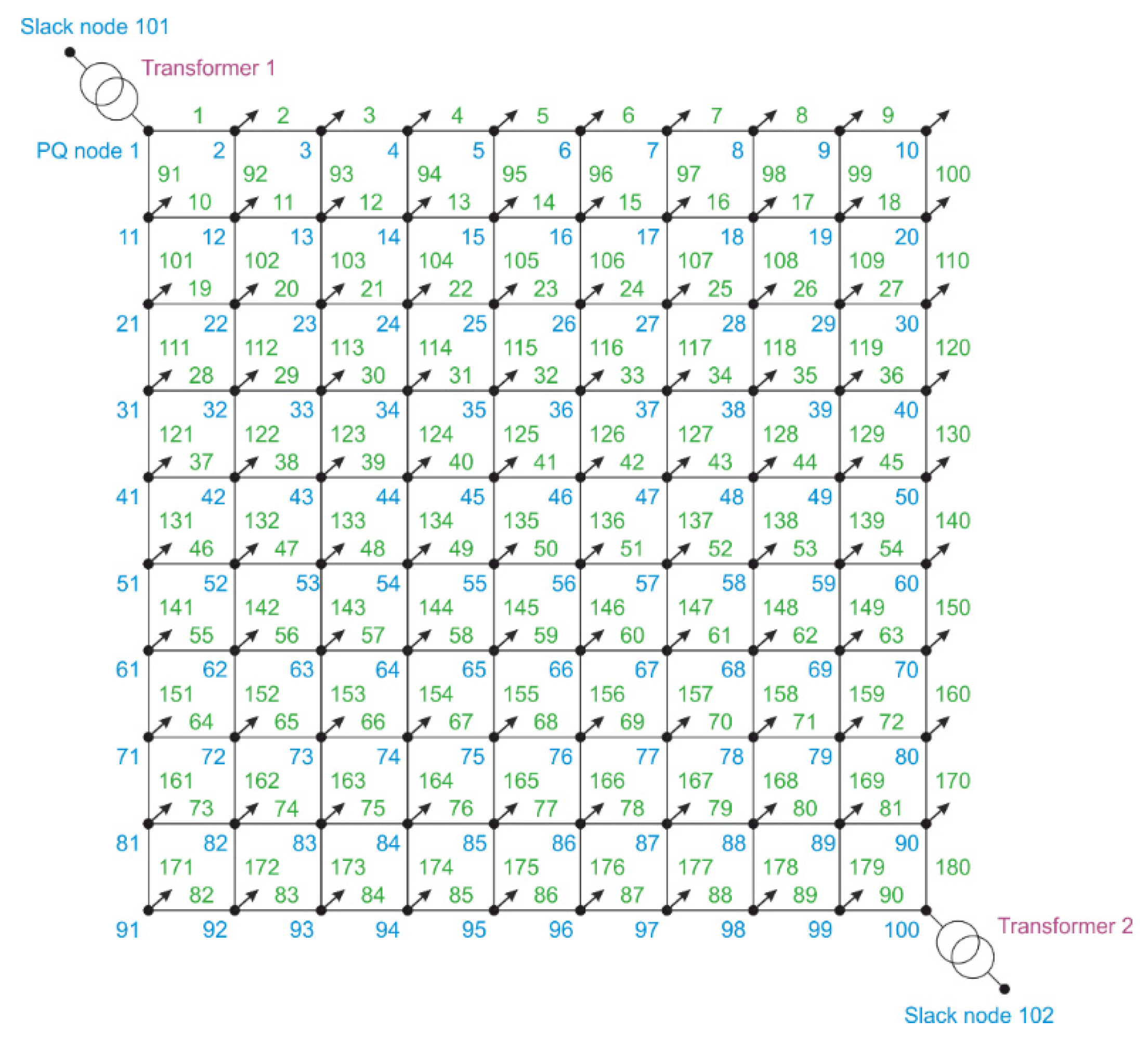
A meshed electrical network from Figure 1 with 100 nodes and 180 power-line sections was used for the tests in this study. In its basic configuration, the tested network model consisted of 100 0.4-kV and 2 22-kV nodes, 2 transformers (each one connected one 22-kV node with one 0.4-kV node), and 180 power-line sections. Its basic structure and parameters were the same for all tests, but in each test, a unique network topology was obtained by switching off some power-line sections. Therefore, each used network topology was described by a combination of power-line sections that were switched off.

Transformers were modelled by the T-equivalent model, and power-line sections were modelled by the π-equivalent model. Each power-line section was realized by the cable CYKY 4 × 50 mm² (its parameters were: the capacitance = 0, the series resistance = 0.39 Ω/km, the series reactance = 0.077 Ω/km). The length of each power-line section was 0.1 km. One active and reactive power consumer was connected in each low-voltage node (there was an exception: in the case of the two 0.4 kV nodes where the transformers were connected, there was no power consumer connected to them). The power consumption of each consumer was P = 6 kW, Q = 1 kvar.

The individual test sets differed from each other only in the number of switched-off power-line sections of the tested network. In the first set, network topologies with one randomly chosen power-line section switched off were tested, in the second set, network topologies with two randomly chosen power-line sections switched off were tested, and so on. Each test set consisted of 100 individual tests, resulting in a total of 15,000 unique tests. Since the test network model consisted of a total of 180 power-line sections and it was necessary to keep a sufficient part of the network model in operation during each test, the maximum value of the number of power-line sections switched off was set to 150. So, the network topologies with the highest number of power-line sections switched off had 150 randomly chosen power-line sections switched off here. Individual combinations of switched-off power-line sections for individual tests were created by a random number generator using a uniform probability distribution. During the combination generation process, if a combination defining the network topology was created that had already been defined earlier in this process, the combination creator deleted the last combination and made a new one.

The local test process had two steps: (1) the test network model was set to the topology that should be tested, and then (2) an AC-power-flow analysis of the model was performed. The current computation time was recorded in the computation time database, and the inserted value described the computation time of the nonlinear solver in seconds (the time spent for editing internal data before and after the AC-power-flow problem solution process was not included in this value). In successfully solved cases, the individual AC-power-flow problem computation processes were terminated when the user’s given tolerance was reached while the tolerance was set so that the difference in the node-apparent-power magnitude had to be lower than 10⁻⁶ for any network node. If the limit of the maximum allowed number of iterations was reached (this limit was set to 100) but the solution was still not found, the case was declared as unsuccessful.

3.2. Results

3.2.1. Speed of Execution

The computation time of each method was the only output data from the individual tests. The value of the computation time corresponds to the time spent in the solver that was used for the test. The time spent for the data type conversions was not considered in this value. If the solution process reached the limit of the maximum allowed number of iterations, which was set as 100, the number 1000 was recorded in the computation time database as the computation time value of the last performed test. Later, during data post-processing, the number 1000 in the database was read as a state where the AC-power-flow problem solution process did not achieve a result within the limit (i.e., it did not reach the correct and acceptable final result).

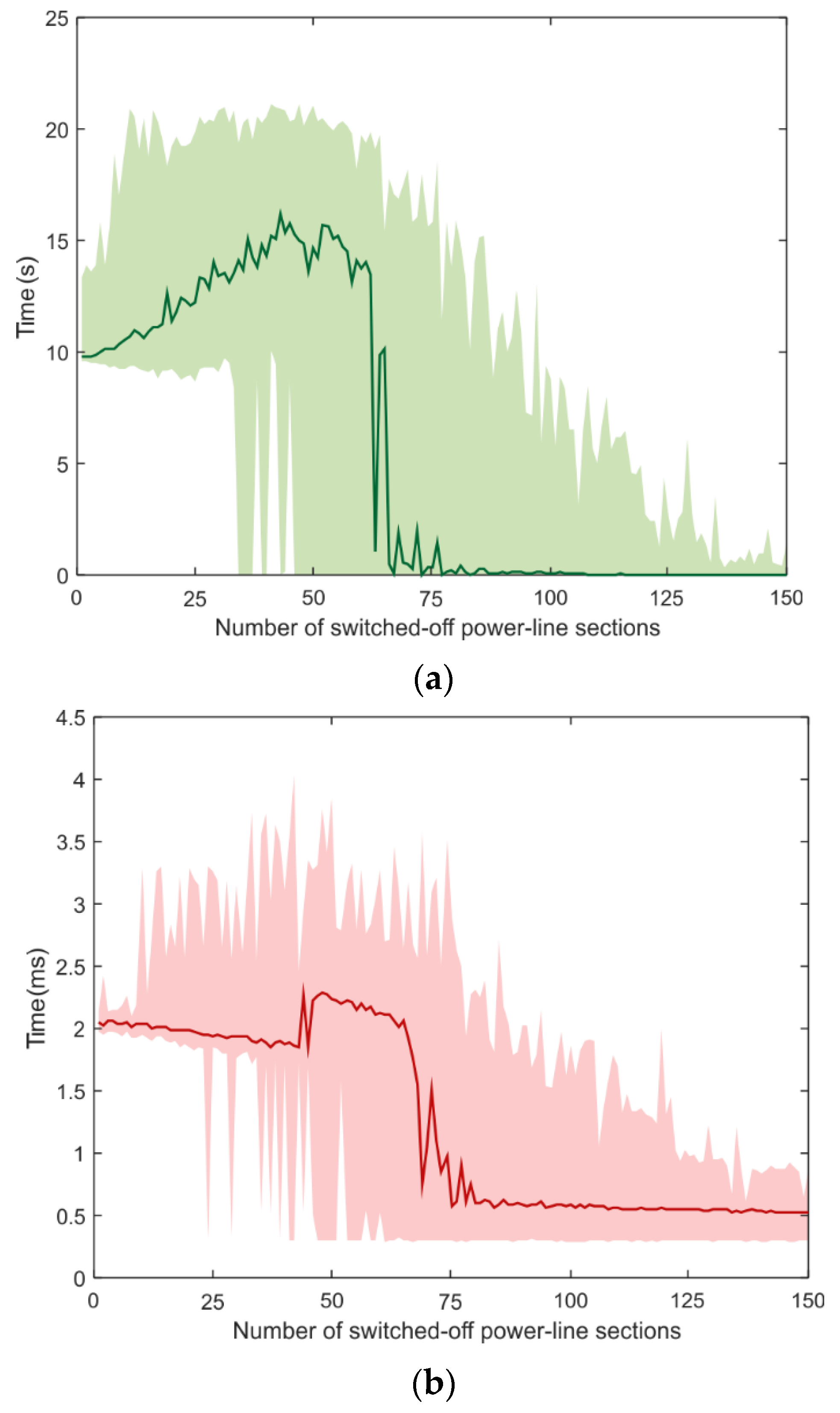
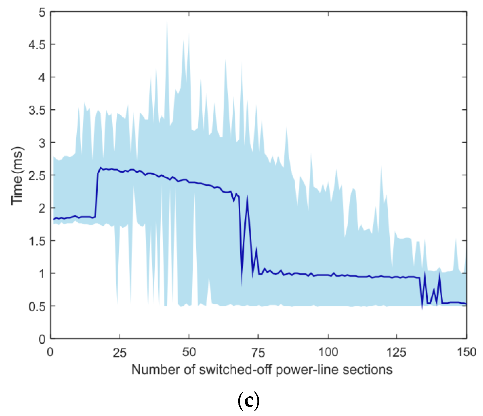
The time of execution for 1000 repeated test cases for the G–S method is given in seconds in Figure 2a, the time of execution for 1000 test cases for the N–R method is given in milliseconds in Figure 2b, and the time of execution for 1000 test cases for the N–R–I method is given in milliseconds in Figure 2c.

The test results say:

• The computation time in the successful convergent cases of the pandapower G–S method implementation is an order of magnitude longer than the computation time of the two other methods, regardless of the network topology, and, therefore, it is the least efficient among the three studied here. Considering the results of all tests performed except the ones where the AC-power-flow analysis solution process did not converge to the solution satisfying the user set tolerance, the median of the computation time is 494.4 ms.
• For any test network topology, the recorded computation time of the pandapower’s N–R–I method implementation is slightly longer than the computation time of the N–R method implementation. For the N–R method implementation, the median of the computation time is 944.5 µs, while for the N–R–I method implementation it is 1490.8 µs.

3.2.2. Robustness

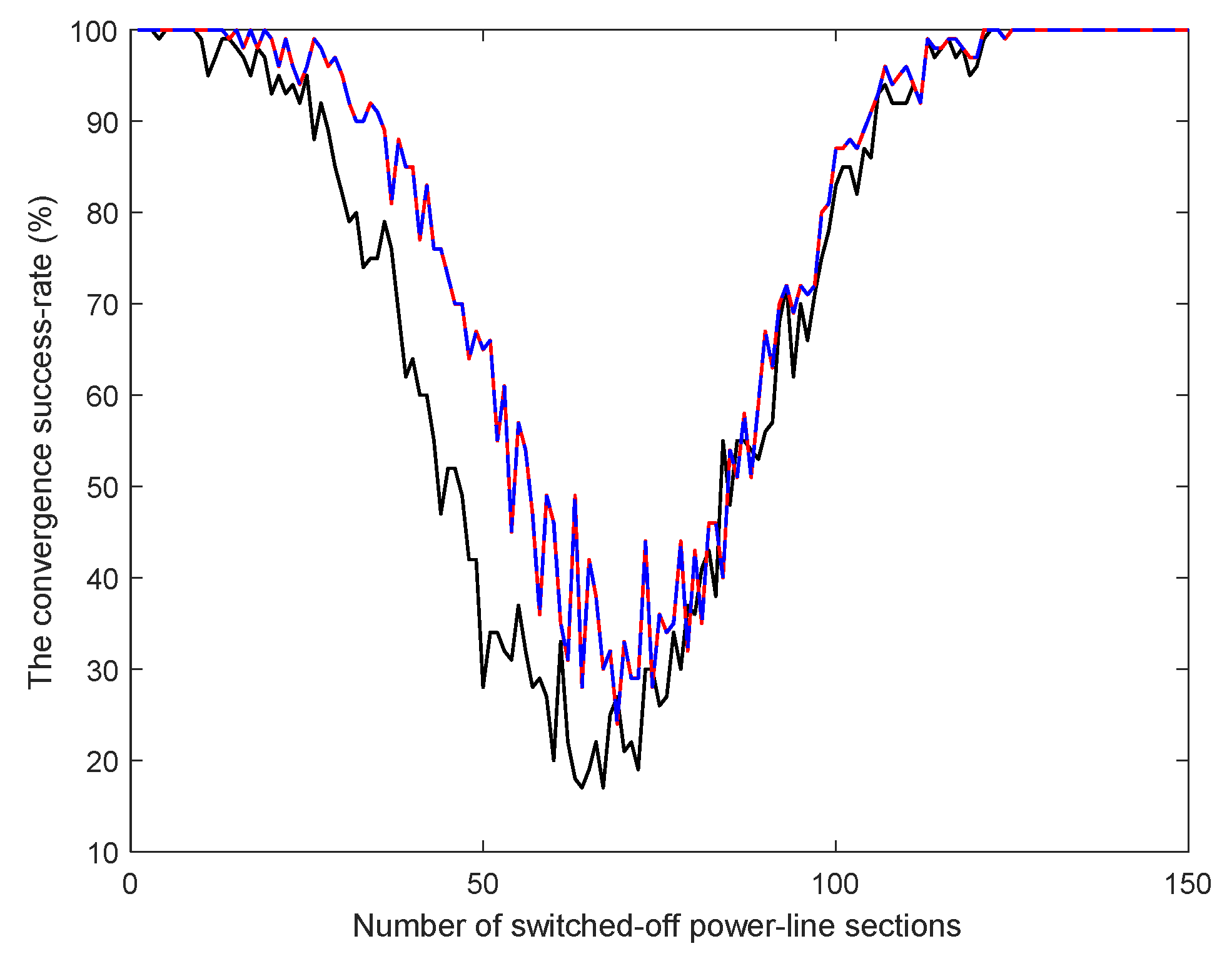
Robustness as the ability of an algorithm to find a solution is measured in this study simply as a percentage of cases in which computation is finished with success. Figure 3 shows the percentage of tests that converged to the solution satisfying the user set tolerance 10⁻⁶.

Regarding successful, convergent cases, the convergence success rate for all methods reaches its highest values for those network topologies where the number of switched-off power-line sections is low (it is in the interval between 1 and 13) or where the number of switched-off power-line sections is large (it is in the interval between 125 and 150). Their convergence success rate reaches 100% because of the relative simplicity of such network topologies or because of the limited number of power-line sections.

In Figure 3, it can be seen that the value of the convergence success rate of the N–R and N–R–I methods is the same for any number of power-line sections switched off (these two iterative numerical methods share many of their algorithms, so their results are expected to be quite similar). It can be also seen that the G–S method is always slightly less robust compared with the N–R and N–R–I methods.

According to Iwamoto and Tamura [5], the introduction of the Iwamoto multiplier into the N–R method’s algorithm was designed to create an AC-power-flow analysis solution method that would be more computationally robust than the basic N–R method. However, in our study, the N–R–I method performance was not higher than the performance of the N–R method. The robustness of these two methods was the same, and the N–R–I method was slower. From the total number of 15,000 combinations of test network topologies, there were only seven sets of topology combinations in which the convergence success rate value was slightly higher for the G–S method than for the N–R and the N–R–I methods (it was for the series of tests when the number of power-line sections switched off was 69, 74, 79, 81, 84, 86, and 88).

Results indicate that convergence success rates for the examined methods strongly depend on the current network topology and the used iterative method:

• G–S method: The convergence success rate reaches the lowest values when the number of switched-off power-line sections is in the interval between 60 and 72 (for the numbers of switched-off power-line sections within this interval, their convergence success rate equals only around 20%, while the quantity’s minimum value is 17% and is reached when the number of switched-off power-line sections is 64 or 67).
• N–R and N–R–I methods: The convergence success rate reaches the lowest values for those network topologies where the number of switched-off power-line sections is in the interval between 62 and 76 (for the numbers of switched-off power-line sections within this interval, their convergence success rate equals only around 30%, while the quantity’s minimum value is 24% and is reached when the number of switched-off power-line sections is 69).

4. Description of New Software Tool—Python Interface between the Pandapower and the SciPy Package with Additional Computational Methods

In the community of developers of software for modelling and control of electrical networks, the pandapower development platform (it is a Python-based function library [28]) is increasingly used. Pandapower is a very capable tool: its user can create a model of any AC power network quickly and easily, and then it can solve the AC-power-flow problems and optimal-power-flow problems, do the state estimates, the topological graph searches [29], and short-circuit calculations according to IEC 60909 [30]. The main competitors of pandapower that perform similar capabilities and features are OpenDSS [31] and Matpower [32].

In addition to an extensive analysis of the three standard AC-power-flow solution methods, the authors of this communication also give a brief analysis of several AC-power-flow solution methods that can be extensively used in the future. The future software for steady-state analysis of electrical networks will very possibly use solvers of SciPy, a Python-based function library. Thanks to the implemented interface between pandapower and SciPy, detailed convergence behavior of various SciPy solvers can be analyzed using Python scripts. A generalized Python interface between the pandapower and SciPy package was used for testing additional methods such as “krylov”, “anderson” [33], “broyden1”, “broyden2” [33], MINPACK’s “hybrd” and “hybrj” routines (modified Powell “hybr” method), and Levenberg–Marquardt “lm” methods. The chart in Figure 4 shows the interconnections between the individual parts of the pandapower–SciPy interface.

At first, the network with all power-line sections switched on was considered, and their solutions were compared to the solution found by the N–R method. The “anderson”, “broyden1”, and “broyden2” methods were unsuccessful in finding the solution to the problem. Hence, the “lm”, “hybr”, and “krylov” methods advanced to the further test, in which the network with 69 power-line sections switched off was assumed (number 69 was chosen as the center point of the interval of a number of power-line sections switched off that gave us the lowest convergence success rate of the N–R method within local analysis). The success rate of the “krylov” and “hybr” method was the same as for the N–R method, i.e., it was 24%. Both methods remained at approximately 0.004 of the error value, but neither of them was able to find a solution in more cases than the N–R method. Only the “lm” algorithm found the solution in all cases that were tested here. However, the AC-power-flow problem solutions provided by the “lm” method were just approximate ones, because the “lm” method is based on the least-square algorithm. Thus, the “lm” method stops its iterative solution process even though it is quite far away from an exact solution of the AC-power-flow problem. The best error value of the “lm” method, which was observed for the series of tests with network topologies with 69 power-line sections switched off, was approximately 0.028. In comparison, the best error value of the N–R method for the same series of tests was approximately 0.006.

Due to the low success rate of the mentioned methods, a quasilinearization method [34] and continuous Newton method [7,35] were implemented into the Python interface script. They were also tested for the case of 69 switched-off power-line sections, but the median value of the observed success rate in this series of tests was lower than the median value observed within the N–R method analysis.

Files with data from tests of these additional methods are given in Supplementary Materials.

5. Conclusions

The test results presented in this paper show that the pandapower implementations of the Newton–Raphson (N–R) method and the Newton–Raphson method with Iwamoto multipliers (N–R–I) have the same superior performances, while the pandapower implementations of the Gauss–Seidel method (G–S) is the least robust of the three tested methods. The AC-power-flow problem solution using the pandapower implementation of the G–S method is more time-demanding than the problem solution using pandapower implementation of the N–R or the N–R–I methods, regardless of the network topology that is used. The N–R–I method has the same performance as the N–R method, but it is slightly more complex. Therefore, from both the efficiency and robustness point of view, the N–R method is the best choice.

Additionally, based on the test results, it can be concluded that all SciPy methods, along with the quasilinearization algorithm, and the continuous Newton method make computations in a short time. However, due to its nature, the results provided by the “lm” method during all local tests deviated greatly from the exact solution of the AC-power-flow problem. So, the analysis results show that the “lm” method is only suitable for those applications of the AC-power-flow solver where only approximate results of the AC-power-flow problem are good enough.

References

- Currie, R.A.; Ault, G.W.; Foote, C.E.; McNeill, N.M.; Gooding, A.K. Smarter ways to provide grid connections for renewable generators. In Proceedings of the IEEE General Meeting Power & Energy Society, Minneapolis, MN, USA, 25–29 July 2010; pp. 1–6. [Google Scholar] [CrossRef]
- Virtanen, P.; Gommers, R.; Oliphant, T.E.; Haberland, M.; Reddy, T.; Cournapeau, D.; Burovski, E.; Peterson, P.; Weckesser, W.; Bright, J.; et al. SciPy 1.0: Fundamental algorithms for scientific computing in Python. Nat. Methods 2020, 17, 261–272. [Google Scholar] [CrossRef] [PubMed] [Green Version]
- Xiao, B.; Zheng, J.; Yan, G.; Shi, Y.; Jiao, M.; Wang, Y.; Dong, L.; Wang, M.; Yang, H. Short-term optimized operation of Multi-energy power system based on complementary characteristics of power sources. In Proceedings of the IEEE Innovative Smart Grid Technologies—Asia (ISGT Asia), Chengdu, China, 21–24 May 2019; pp. 1–6. [Google Scholar] [CrossRef]
- Tur, M.R.; Bayindir, R. A review of active power and frequency control in smart grid. In Proceedings of the 1st Global Power, Energy and Communication Conference (GPECOM), Nevsehir, Turkey, 29 July 2019; pp. 1–6. [Google Scholar] [CrossRef]
- Iwamoto, S.; Tamura, Y. A load flow calculation method for ill-conditioned power systems. IEEE Trans. Power Appar. Syst. 1981, PAS-100, 1736–1743. [Google Scholar] [CrossRef]
- Le Nguyen, H. Newton-Raphson method in complex form [power system load flow analysis]. IEEE Trans. Power Syst. 1997, 12, 1355–1359. [Google Scholar] [CrossRef]
- Milano, F. Continuous Newton’s method for power flow analysis. IEEE Trans. Power Syst. 2009, 24, 50–57. [Google Scholar] [CrossRef]
- Dolgicers, A.; Kozadajevs, J. Phase plane usage for convergence analysis of Seidel method applied for network analysis. In Proceedings of the 2014 IEEE 2nd Workshop on Advances in Information, Electronic and Electrical Engineering (AIEEE), Vilnius, Lithuania, 28–29 November 2014; pp. 1–6. [Google Scholar] [CrossRef]
- Chatterjee, S.; Mandal, S. A novel comparison of Gauss-Seidel and Newton-Raphson methods for load flow analysis. In Proceedings of the International Conference on Power and Embedded Drive Control (ICPEDC), Chennai, India, 16–18 March 2017; pp. 1–7. [Google Scholar] [CrossRef]
- Gharebaghi, S.; Safdarian, A.; Lehtonen, M. A linear model for AC power flow analysis in distribution networks. IEEE Syst. J. 2019, 13, 4303–4312. [Google Scholar] [CrossRef]
- Foltyn, L.; Vysocký, J.; Prettico, G.; Běloch, M.; Praks, P.; Fulli, G. OPF solution for a real Czech urban meshed distribution network using a genetic algorithm. Sustain. Energy Grids Netw. 2021, 26, 100437. [Google Scholar] [CrossRef]
- Lohmeier, D.; Cronbach, D.; Drauz, S.R.; Braun, M.; Kneiske, T.M. Pandapipes: An open-source piping grid calculation package for multi-energy grid simulations. Sustainability 2020, 12, 9899. [Google Scholar] [CrossRef]
- Brkić, D.; Praks, P. Short overview of early developments of the Hardy Cross type methods for computation of flow distribution in pipe networks. Appl. Sci. 2019, 9, 2019. [Google Scholar] [CrossRef] [Green Version]
- Brkić, D.; Praks, P. An efficient iterative method for looped pipe network hydraulics free of flow-corrections. Fluids 2019, 4, 73. [Google Scholar] [CrossRef] [Green Version]
- Brkić, D. An improvement of Hardy Cross method applied on looped spatial natural gas distribution networks. Appl. Energy 2009, 86, 1290–1300. [Google Scholar] [CrossRef] [Green Version]
- Brkić, D. Discussion of “Economics and statistical evaluations of using Microsoft Excel solver in pipe network analysis”. J. Pipeline Syst. Eng. Pract. 2018, 9, 07018002. [Google Scholar] [CrossRef] [Green Version]
- Jha, K.; Mishra, M.K. Object-oriented integrated algorithms for efficient water pipe network by modified Hardy Cross technique. J. Comput. Des. Eng. 2020, 7, 56–64. [Google Scholar] [CrossRef]
- Rai, R.K.; Lingayat, P.S. Analysis and design of urban water distribution network using Hardy Cross method and EPANET. In Advances in Civil Engineering and Infrastructural Development; Springer: Singapore, 2021; pp. 347–357. [Google Scholar] [CrossRef]
- Niazkar, M.; Eryılmaz Türkkan, G. Application of third-order schemes to improve the convergence of the Hardy Cross method in pipe network analysis. Adv. Math. Phys. 2021, 2021, 6692067. [Google Scholar] [CrossRef]
- Khan, W.A. Numerical and simulation analysis comparison of hydraulic network problem base on higher-order efficiency approach. Alex. Eng. J. 2021, 60, 4889–4903. [Google Scholar] [CrossRef]
- Novitsky, N.; Mikhailovsky, E. Generalization of methods for calculating steady-state flow distribution in pipeline networks for non-conventional flow models. Mathematics 2021, 9, 796. [Google Scholar] [CrossRef]
- da Silva Teixeira, G.; Alonso, G.V.; Mendes, L.J. Evaluation of nonlinear iterative methods on pipe network. Ing. Mecánica 2021, 24, e625. Available online: https://ingenieriamecanica.cujae.edu.cu/index.php/revistaim/article/view/656 (accessed on 21 October 2021).
- Cross, H. Analysis of Flow in Networks of Conduits or Conductors. University of Illinois at Urbana Champaign, College of Engineering. Engineering Experiment Station. 1936. Available online: http://hdl.handle.net/2142/4433 (accessed on 21 October 2021).
- Ramkhelawan, R.; Musti, K.S. Power system load flow analysis using Microsoft Excel–Version 2. Spreadsheets Educ. 2019, 12, 11006. Available online: https://sie.scholasticahq.com/article/11006 (accessed on 21 October 2021).
- Stott, B.; Alsac, O. Fast decoupled load flow. IEEE Trans. Power Appar. Syst. 1974, PAS-93, 859–869. [Google Scholar] [CrossRef]
- Tostado-Véliz, M.; Kamel, S.; Jurado, F. A robust power flow algorithm based on Bulirsch–Stoer method. IEEE Trans. Power Syst. 2019, 34, 3081–3089. [Google Scholar] [CrossRef]
- Pourbagher, R.; Derakhshandeh, S.Y. Application of high-order Levenberg–Marquardt method for solving the power flow problem in the ill-conditioned systems. IET Gener. Transm. Distrib. 2016, 10, 3017–3022. [Google Scholar] [CrossRef]
- Thurner, L.; Scheidler, A.; Schäfer, F.; Menke, J.H.; Dollichon, J.; Meier, F.; Meinecke, S.; Braun, M. Pandapower—An open-source python tool for convenient modeling, analysis, and optimization of electric power systems. IEEE Trans. Power Syst. 2018, 33, 6510–6521. [Google Scholar] [CrossRef] [Green Version]
- Xiao, R.; Xiang, Y.; Wang, L.; Xie, K. Power system reliability evaluation incorporating dynamic thermal rating and network topology optimization. IEEE Trans. Power Syst. 2018, 33, 6000–6012. [Google Scholar] [CrossRef]
- Sweeting, D. Applying IEC 60909, fault current calculations. IEEE Trans. Ind. Appl. 2011, 48, 575–580. [Google Scholar] [CrossRef]
- Montenegro, D.; Hernandez, M.; Ramos, G.A. Real time OpenDSS framework for distribution systems simulation and analysis. In Proceedings of the Sixth IEEE/PES Transmission and Distribution: Latin America Conference and Exposition (T&D-LA), Montevideo, Uruguay, 3–5 September 2012; pp. 1–5. [Google Scholar] [CrossRef]
- Zimmerman, R.D.; Murillo-Sánchez, C.E.; Thomas, R.J. MATPOWER: Steady-state operations, planning, and analysis tools for power systems research and education. IEEE Trans. Power Syst. 2010, 26, 12–19. [Google Scholar] [CrossRef] [Green Version]
- Eyert, V. A comparative study on methods for convergence acceleration of iterative vector sequences. J. Comput. Phys. 1996, 124, 271–285. [Google Scholar] [CrossRef]
- Nagrial, M.H.; Soliman, H.M. Power flow solution using the modified quasilinearization method. Comput. Electr. Eng. 1984, 11, 213–217. [Google Scholar] [CrossRef]
- Milano, F. Analogy and convergence of Levenberg’s and Lyapunov-based methods for power flow analysis. IEEE Trans. Power Syst. 2015, 31, 1663–1664. [Google Scholar] [CrossRef]