Article

A Mixed Ensemble Learning and Time-Series Methodology for Category-Specific Vehicular Energy and Emissions Modeling

Department of Civil Engineering, McGill University, Montreal, QC H3A 0C3, Canada
*
Author to whom correspondence should be addressed.
Sustainability 2022, 14(3), 1900; https://doi.org/10.3390/su14031900
Submission received: 15 November 2021 / Revised: 14 January 2022 / Accepted: 28 January 2022 / Published: 7 February 2022
(This article belongs to the Topic Big Data and Artificial Intelligence)

Abstract

:
The serially-correlated nature of engine operation is overlooked in the vehicular fuel and emission modeling literature. Furthermore, enabling the calibration and use of time-series models for instrument-independent eco-driving applications requires reliable forecast aggregation procedures. To this end, an ensemble time-series machine-learning methodology is developed using data collected through extensive field experiments on a fleet of 35 vehicles. Among other results, it is found that Long Short-Term Memory (LSTM) architecture is the best fit for capturing the dynamic and lagged effects of speed, acceleration, and grade on fuel and emission rates. The developed vehicle-specific ensembles outperformed state-of-the-practice benchmark models by a significant margin and the category-specific models outscored the vehicle-specific sub-models by an average margin of 6%. The results qualify the developed ensembles to work as representatives for vehicle categories and allows them to be utilized in both eco-driving services as well as environmental assessment modules.

1. Introduction

Training meso- and micro-scale models for estimating vehicular Fuel Consumption Rate (FCR) and Emission Rates (ER) is a fundamental step towards developing reliable eco-driving assistance services. Such models could also be used as a part of environmental-assessment modules in the existing traffic simulation software. The micro-scale models focus on understanding instantaneous correlations between the state of the vehicle and the fuel and emission rates. They provide richer information for transportation environmental analysis.
The existing micro-scale fuel and emission models suffer from five major issues. First, many of them depend on Internal Engine Variables (IEV) to achieve acceptable levels of accuracy [1,2,3,4,5,6,7], which eliminates their applicability in instrument-independent eco-driving services or integration with traffic simulation models.
Second, some of the popular comprehensive models such as MOVES [8] and CMEM [9] require multiple processing steps that do not allow their real-time use. Some efforts have been made to tackle this problem by pre-running various scenarios and generating multi-dimensional matrices for fuel and emission rates [10]; nevertheless, deploying such models is still computationally expensive.
Third, the existing research-based and commercial models could not be used in countries other than those of their origin. However, as some counter examples, the American MOVES model is being widely used in Canada or the European COPERT IV [11] and LEAP [12] models are being used in South America. As a result, their predictions could be biased due to the differences in the fleet, driving-habits, meteorology, road conditions, etc.
Our real-world evaluation in Canada [13] revealed that MOVES underestimates energy consumption and Carbon Dioxide (CO2) rates by 17% and 35%, respectively. A dramatic overestimation (up to 420%) was observed for Nitrogen Oxides (NOx) and Particulate Matters (PM) predictions as well.
Fourth, the time-series and more importantly, the serially-correlated nature of the engine operation is rarely addressed in the literature. The temporally extended impact of past driving events (a few seconds before time t ) on current fuel and emission rates is either left unobserved [1,2,4,7,14,15], acknowledged but disregarded and considered effectless [16], or at best is spread through time as an error using moving average techniques to improve instantaneous predictions [3,5].
Fifth and last, methodologies for generalization and aggregation of the vehicular fuel and emission models are missing in the literature. Robust models capable of accurately forecasting FCR and ERs without the need for parametric calibration for specific vehicle characteristics would have a wider range of use cases in practice.
We evaluated and attempted to solve the first three of the abovementioned issues in our two previous publications [13,17]. In this study, we focus on finding solutions for the last two issues. The novelty of our approach could be summarized as:
(1)
To achieve acceptable prediction accuracies in the absence of precise engine-state measurements (a requirement for instrument-independent models) while addressing the serial correlation and the lagged impact of variables on FCR and ERs, we utilize a state-of-the-art Machine Learning (ML) technique of Recurrent Neural Networks (RNN) to keep the models’ architecture in alignment with the nature of the observed vehicular operation data.
(2)
The fact that the order of lagged effects of variables on FCR and ERs is not necessarily constant has never been questioned in the literature. Hence, we use an Ensemble Learning (EL) approach to tackle such uncertainty and dynamicity.
(3)
Unlike the vast majority of the previous studies that are confined to vehicle-specific modeling, we consider the need for category-specific FCR and ER models; hence, we introduce a generalization methodology (from vehicles to categories) founded upon well-recognized forecast-combination techniques.
The rest of the paper is structured as follows: In Section 2, some of the notable studies and commercial efforts on microscale fuel consumption and emission modeling are reviewed. Section 3, explains our methodology for RNN time-series modeling and introduces a two-step EL approach for generalizing the vehicle-specific models to category-specific ones. The modeling results are then visually and statistically analyzed and discussed in Section 4. At the end, in Section 5, conclusions are drawn and possible future research topics following this study are depicted.

2. Literature Review

In addition to the commercial models, there have been several academic studies on development of microscale FCR and ER estimation models. They range from 0D/1D approaches (physicochemical simulation) to the use of traditional statistical techniques such as multivariate linear/nonlinear regression, and finally, taking advantage of emerging ML algorithms such as Support Vector Machines (SVM) and Artificial Neural Networks (ANN).
Although providing accurate predictions, the sensitivity of the performance of 0D/1D models [15,18,19,20,21,22] to the accuracy of input variables is a matter of concern. This family of models is complex and mostly benefits from the IEVs. This makes them instrument-dependent and therefore, limits their real-world applications.
Cascaded techniques are proposed in the literature to reduce the complexity of the fuel and emission models. For instance, equilibrium concentrations of oxygen and nitrogen during NOx formation in the combustion chamber are calculated by injecting IEV measurements into the Zeldovich model [23,24] and the resulting estimates are used to predict the NOx rate [3].
By the introduction of Virginia Tech’s Comprehensive Power-based Fuel Model (VT-CPFM), a significant step was taken towards pure data-driven fuel- and emission-rate modeling [5,25]. The model uses nonlinear polynomial regression and estimates of power demand as a proxy variable. However, the IEV-independent version of the model, VT-CPFM Type I, cannot compete with the state-of-the-art ML models developed later [17].
Stepping into ML modeling in the recent few years, simple neural network architectures are widely used in the literature to estimate fuel and emission rates for the cold-start, hot-start, and hot-stabilized engine conditions [26,27,28,29]. However, sophisticated techniques capable of capturing serial correlation and lagged effects of variables are overlooked. Moreover, independence from IEVs is not prioritized in many of the studies, which dramatically limits the scope of applicability of the developed models.
As the second part of a series of studies, we started with the validation of predictions by EPA’s comprehensive emissions model, MOVES [13], we introduced a cascaded machine-learning methodology for FCR estimation using large amounts of data collected through on-road measurements [17]. In that study, the absence of influential IEVs such as Engine Speed (RPM) was compensated for by using their estimates. As a result, the accuracy of models reached 83%, while improvements as high as 37% were achieved compared to using an IEV-free variable set. In addition, our assessment of the direct use of lagged variables in SVR and ANN algorithms proved the weakness of these methods in capturing serially correlated and lagged effects of variables on FCR, emphasizing the need for a transition to more innovative ML algorithms.
Time alignment of the input data is a popular method of dealing with lags and autocorrelation [30,31]. Even the U.S. Environmental Protection Agency (EPA) used the same method for preprocessing the data while estimating MOVES core models. Nevertheless, the approach raises criticism as the lagged effects may not occur with a constant order.
The time-series forecasting of the vehicular FCR and ERs is a challenging problem due to the dynamicity and non-stationarity characteristics of data [32,33,34]. Volatility in variables leads to increased forecasting error and when combined with lagged effects, the majority of the traditional statistical modeling techniques fail to perform acceptably.
RNNs are gaining renewed interest among researchers as they provide promising results for modeling time-series and serially-correlated phenomena [33]. This family of ML algorithms is being widely used in the transportation engineering context; however, they have a pale footprint in vehicular energy and emissions modeling. Most of the studies focus on predicting traffic-flow attributes such as travel-time, volume, speed, etc., or travel-mode and incident detection. For instance, the effect of upstream and downstream speed- and occupancy-rate fluctuations on traffic flow prediction is analyzed using Long Short-Term Memory (LSTM) recurrent neural networks [35]. Moreover, stacked LSTM architectures are evaluated for traffic flow predictions based using historical daily traffic patterns and weather variations [36]. In a more recent simulation-based research, short-term speed of vehicles is predicted using a combination of Convolutional Neural Networks (CNN) and Bidirectional Long Short-Term Memory (Bi-LSTM). The CNN is used to capture the local variations of features, while the Bi-LSTM handling the extended temporal relationships [37]. Such studies have proved the exceptional power of RNNs in capturing temporally-distributed effects, even with a limited number of input variables. Creative solutions relying on RNN algorithms have simplified mode-detection process using smartphone sensor measurements [38] as higher accuracy could be achieved with RNNs even with lower-resolution input data, making the models’ execution computationally inexpensive. The use cases of RNN algorithms were recently expanded to classification and pattern recognition. Road anomaly detection from the perspective of a vehicle is conducted using RNNs with the physical road characteristics as time-series and serially-correlated inputs to the models [39]. Moreover, improving near-future travel-time predictions based on historical data and real-time sensor observations are frequently addressed in the transportation literature. It is interesting that almost all of the recently proposed models rely on innovative combinations of RNN techniques [40,41,42,43,44,45,46]. In a rare case, RNN technique is introduced to the vehicular FCR modeling literature as well [47]; however, the generalization of the developed model is questionable due to use of a single vehicle for experiments.
The capacity of the modeling methodology to allow generalization to more aggregate levels is an important factor when developing vehicular fuel and emission models either for eco-driving purposes, use in traffic simulations, or even for large-scale environmental assessments in transportation planning. For the purpose of generalization, several forecast combination techniques are introduced in the traditional statistics literature including methods of Simple Averaging [48] and the Trimmed and Winsorized means [49]. These methods underperform significantly when the distribution of data is skewed [32]. An alternative option frequently used by scholars for ensemble learning is the Ordinary Least Squares (OLS) regression [50,51,52].
Forecast combination algorithms have been going through an evolution in recent years. Methods founded upon the concepts of Decision Trees (DT), Gradient Boosting (GB) and its extensions such as AdaBoost (AB), Random Forests (RF), SVM, and even ANN have come into focus of the ensemble modelers and have proved their capability in generating significantly improved predictions [53,54].
Elucidating the goals of this study, we will try to assess the feasibility of using popular EL techniques as means of deriving robust category-specific FCR and ER models from vehicle-specific IEV-independent RNN models. Such an approach opens avenues to simpler and faster development of accurate fleet-specific models with diverse use cases in the transportation field.

3. Methodology

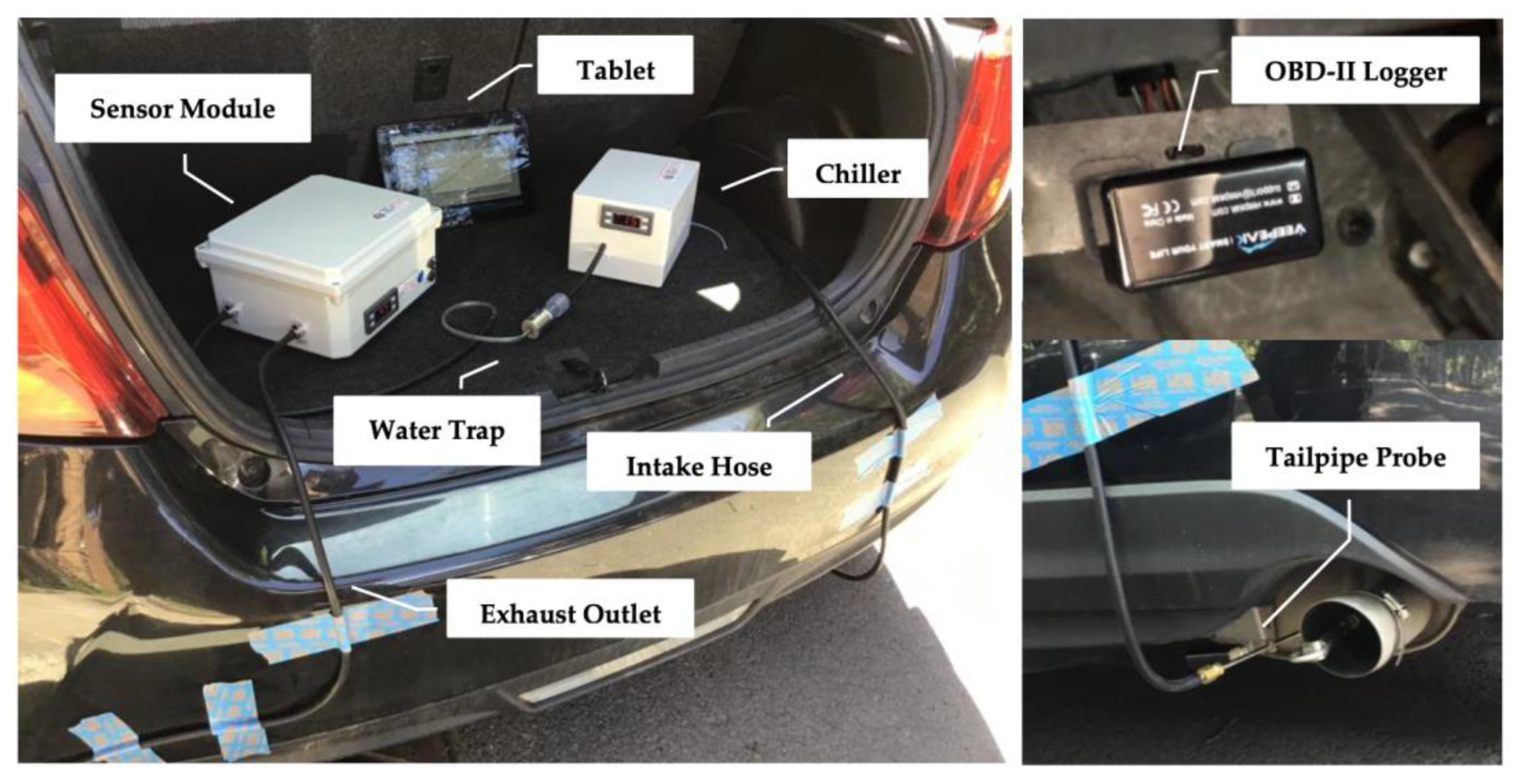
3.1. On-Road Experiments

The test fleet for on-road experiments included 35 different passenger cars from three cities of Montreal (Canada), Bucaramanga (Colombia), and Tehran (Iran). On-Board Diagnostics (OBD) loggers installed on the vehicles collected the engine-state parameters. Instantaneous GPS coordinates and accelerometer measurements were logged simultaneously. The OBD parameter set included RPM, Manifold Absolute Pressure (MAP), Mass Air Flow (MAF), Barometric Pressure (P), Fuel-Air Equivalence ratio ( ϕ ), and Intake Air Temperature (IAT). A state-of-the-technology Portable Emissions Measurement System (PEMS) was installed on the tailpipe of vehicles under study in Montreal to monitor and log the instantaneous CO2, PM, Nitrogen Monoxide (NO), and Nitrogen Dioxide (NO2) concentrations.
The PEMS measures CO2 using Non-Dispersive Infra-Red (NDIR) absorption technology with a measurement range of 0–20% and an accuracy of ±70 ppm. For the NOx, 3-electrode electrochemical sensors capable of measuring up to 5000 ppm for NO and 300 ppm for NO2 were incorporated. The measurement resolution for NO and NO2 were 1–5 ppm and 0.1 ppm, respectively. Regarding PM, the unit measures undiluted emissions through the response of three dissimilar particulate sensors. Ionization was used for ultra-fine/fine particulates usually between 0.01 to 1 micron, while a combination of opacimeter and laser scattering was deployed for coarse particulates up to 10 microns.
It is important to note that we performed activity and fuel rate data collection on all 35 vehicles under study. However, the additional tailpipe emission measurement was conducted only on 17 vehicles all from Montreal.
Figure 1 shows both of the sensors installed on a test vehicle. The intake probe clamped to the tailpipe collects exhaust sample at a rate of 2.5 L/min. As there was no dilution, no extrapolation of the sensor values to the full concentrations was required. A chiller unit condenses and removes the water vapor present in the exhaust. An additional water trap completes the water-removal process before sending the sample to the main unit.
Cold-start emissions were disregarded in this study as the sensing process started after reaching the hot-stabilized engine operation. Pre- and post-test ambient emission levels were measured and used as a reference for calculating the net exhaust emission concentrations.
The maintenance quality of the vehicles was evaluated through interviews with the volunteer car owners participating in the experiments. Vehicles with uncertain/unacceptable conditions were excluded. A single person drove all the cars in each of the three cities. The three drivers coordinated in advance in terms of driving style to mitigate the chance of bias in sampling. The drivers were all asked to avoid aggressive driving and keep their speed coordinated to that of traffic flow. It is noteworthy that the impact of the traffic flow and traffic control systems would be implicitly captured in time-series logs of speed and acceleration.
A driving plan was set in advance for the time-windows drivers had to perform the experiments and to guide them through the road network. The route-map and the time-tables obliged them to drive approximately 30% of the time on highways, 30% on arterials, 30% on local roads, while dedicating the remaining 10% of the time to uphill and downhill driving. The equivalent distance for the above shares varied in each test. However, as the FCR and ERs are time-based, time was selected as a reference for scheduling the trip-chain plans. For the 10% uphill- and downhill-driving time-window, special road segments with grades beyond normal road design thresholds (higher than 7% or less than −7%) were targeted. By taking such an approach, the randomness of data in terms of speed, road grade, and diversity of acceleration/deceleration patterns was preserved.
Figure 2 presents the aggregated view of GPS trajectories for experiments conducted in Montreal and Bucaramanga. Moreover, Table 1 provides descriptive information about the on-road experiments and Table 2 describes the test fleet specifications.

3.2. Data Preparation

Both the GPS as well as the Inertial Measurement Unit (IMU) output included outliers and noise. To remove the outliers, first, an outlier removal procedure based on Kalman Filtering algorithm [55] was applied. Then, the Savitzky-Golay smoothing algorithm [56] was used to remove noise and minor fluctuations. The algorithm generated more satisfying results compared to other available algorithms such as moving average, exponential, and convolutional smoothing methods. Note that wheel speed retrieved from ECU was prioritized over GPS speed due to relatively higher accuracy. Hence, no post-processing (outlier filtering and smoothing) was applied to instantaneous speed data.
F C R t was calculated indirectly with the help of the observed (Equation (1)) or estimated (Equation (2)) value of the M A F t rate. M A F t represents the flow of air entering a fuel-injected internal combustion engine. Although all modern vehicles were equipped with a MAF sensor, not all of them reported this parameter through the OBD-II interface. M A F t could be acceptably estimated based on M A P t as well.
F C R t = M A F t λ × A F R s t o i c h
M A F t = R P M 120 × M A P t I A T t × V E 100 × E D × M M R
In Equations (1) and (2), index t indicates the instantaneous nature of observations, F C R t and   M A F t are both in g / s , and A F R s t o i c h denotes the air-to-fuel mixture ratio at the stoichiometric level. λ is the actual air-to-fuel ratio (AFR) to its stoichiometric level [57], R P M is in revolutions per minute, M A P t is the pressure at the intake air manifold in kPa , and V E is the volumetric efficiency, which is around 65% for regular gasoline engines and goes up to 85% for turbocharged models. E D denotes engine displacement in Liters, M M is the average molecular mass of air ( 28.97   g / mol ), I A T t is the intake air temperature in Kelvin, and R is the ideal gas constant equal to 8.314   J / ° K / mol .
The PEMS setup reported instantaneous emission concentrations in percentage for CO2, ppm for NOx, and micrograms / m 3 for particulate matters. To convert second-by-second concentrations into temporal rates in the absence of exhaust flow rate data, an all-in all-out assumption was made (ignoring the existence of minor leakage from the engine to the exhaust pipe) and the MAF rate was used as an alternative to the exhaust flow rate. However, the exhaust-pipe lag (due to its length and presence of resonators and catalytic converter) could introduce errors to the calculations. Later in this section, an RNN modeling approach is described as a solution for capturing such lagged effects.
Equations (3) and (4) were used to unify concentration units and adjust the concentrations for prevailing temperature and pressure. The concentrations were then converted to instantaneous emission rates using Equation (5).
F o r   C O 2 : C o n c p p m = 10 6 × C o n c %
C o n c m g / m 3 = C o n c p p m × ( M o l e c u l a r   W e i g h t   o f   G a s 22.4 ) × ( 273 273 + T ) × ( 10 × P 1013 )
E R t = C o n c m g / m 3 × 10 6 × M A F t × ( 10 3 A i r   D e n s i t y )
In Equation (4), T is the intake air temperature in ° C and P is the ambient barometric pressure in kPa . In Equation (5), M A F t is the mass air flow in g / s and the air density is equal to 1.2929   kg / m 3 . The molecular weight of emissions are 44.01, 46.01, and 30.01 g / mol for CO2, NO2, and NO, respectively.
The multiple steps of data collection and preparation procedure are shown in Figure 3 in form of a flowchart. At the bottom layer of the flowchart, the input to the modeling steps explained in the next sections is prepared.

3.3. Vehicle-Specific RNN Modeling

The exhaust-pipe lag is not the only source of lag that affects the vehicular fuel or emission rates. There is a Sensor response delay due to use of electrochemical sensors in the PEMS unit. Such sensors have a slow response time to the changes of emission concentrations. There is also an Engine response delay defined as the lag between the moment a driver takes an action to increase, decrease, or stop the power demand and the moment the engine starts to react. Finally, there is a Kinematic distributed lag as a result of the gradual increase in the vehicle speed towards a target speed (when accelerating) despite instantaneous consumption of the fuel after the driver pushes on the gas pedal.
Although it is possible to qualitatively rank different sources regarding their impact on total order of lag, with the non-destructive experimenting approach taken in this study (we avoided making any modifications to the test vehicles), there is no way to clearly quantify the shares of each source. Hence, in this study, the focus was only on the total order of lag.
Recurrent neural networks are designed to recognize patterns and temporally-distributed effects on the dependent variable in sequences of data, such as time-series. Nevertheless, RNNs are rarely used in the vehicular fuel and emission rate modeling literature. In the vast majority of studies in this field, data points are assumed random samples rather than serially-correlated time-series.
A fully-connected neural network takes in a fixed-size vector and gains no knowledge about temporal interactions between the dependent and the explanatory variables through the training process. However, an RNN model takes the vector of input variables at time t as well as the measurements of up to p lag steps ( t 1 , t 2 , …, t p ) simultaneously into account.
Figure 4 depicts the internal structure of three different RNN cell structures as well as the architecture of a many-to-one RNN model with multiple stacked layers. The many-to-one architecture is an appropriate choice for vehicular fuel and emission modeling as we target a single variable and not a sequence as the prediction output.
Note that X t = [ X t p ,   , X t 2 ,   X t 1 , X t ] is the input matrix corresponding to time t . Each X i element is a columnar vector holding the instantaneous values of the main model variables. In our case, X i would be equal to [ v i , a i , z i ] T , where v i is speed in km / h   , a i is acceleration in m / s 2 , and z i is the GPS altitude in m . The measured instantaneous FCR (or one of the ER values) at time t would be used as the dependent variable ( Y t ).
The temporally extended effects within time-series sequences of each variable were implicitly captured by the gated structure of the RNN cells, while the direct correlations between variables and the dependent at any time step t was modeled by 100-hidden-unit sub-models inside each RNN cell wherever a Sigmoid or Tanh gate exists. In other words, each gate (shown as yellow boxes inside the cell structures in Figure 4a–c) will itself be a fully-connected neural network with 100 activation units. The input to the gates was different for each of the cell structures. In Simple cells, the variables vector X t and a hidden state vector h t are injected into a single tanh gate. The hidden state carries information about the short-term past state of the system. In a LSTM cell, three sigmoid and one tanh gate work together [33,58,59,60,61]. The extra gates and a more complex internal mechanism allow the LSTM cell to manage a memory of the past events at both short- and long-term scales (in addition to the hidden state h t , a cell-state stream of information C t carries long-term memories and the combination of the gates let the cell keep or forget all or a part of the memory). Finally, the Gated Recurrent Units (GRU) are a more recent type of RNN cell structures [62,63]. The RNN architectures founded upon GRU cells have less parameters to be trained; hence, the model will become less computationally expensive both at the training and the execution stages compared to LSTM.
The prediction power of RNNs could be boosted by deepening them through stacking the layers over each other. In a stacked many-to-one RNN architecture, each layer (except the last one) outputs a sequence of vectors which will be used as an input to a subsequent layer. The additional layers are understood to recombine the learned representation from prior layers and create new representations at high levels of abstraction.
As a foundation for developing category-specific models, vehicle-specific RNN models are first estimated for FCR and ERs. Single-, double-, and triple-layer stacked architectures are assessed (deeper structures are disregarded due to the exponentially increasing processing time). Depending on the lag order, data are converted into p-length sets of vectors, and five-fold cross-validation (with 70% of data for training and 30% for validation) is used to achieve robust modeling results.
Regularization is applied through the Dropout technique with a drop probability of 50%. Using this technique, randomly selected neurons are ignored during each training iteration. Hence, the contribution of the ignored neurons to the activation of downstream neurons is temporally removed on the forward pass and any weight updates are not applied to the neuron on the backward pass. Therefore, other neurons will have to step in and handle the representation required to make predictions for the missing neurons. As a result, the neural network is allowed to learn multiple independent internal representations and it becomes capable of better generalization and will be less likely to overfit the training data.
Mean Normalization is applied for feature scaling before training on the target variables of speed, acceleration, and the GPS altitude as well as the dependent variable (either the FCR or one of the ERs). The variables will be rescaled so that they will have the properties of a standard normal distribution. Feature scaling is recommended in ML to avoid attributes in greater numeric ranges (such as speed or altitude) dominating those in smaller numeric ranges (such as acceleration). Furthermore, feature scaling speeds up the gradient descent convergence during the training process of the ML models, especially when the data has high variance.
Mean Squared Error (MSE) is used as the loss function, and the Adam algorithm is considered for the neural network’s optimization (due to faster convergence compared to Momentum, RMSprop, and Stochastic Gradient Descent algorithms). Python programming language as well as two popular ML libraries of TensorFlow [64] and Scikit-Learn [65] are used for training and evaluation of the models.

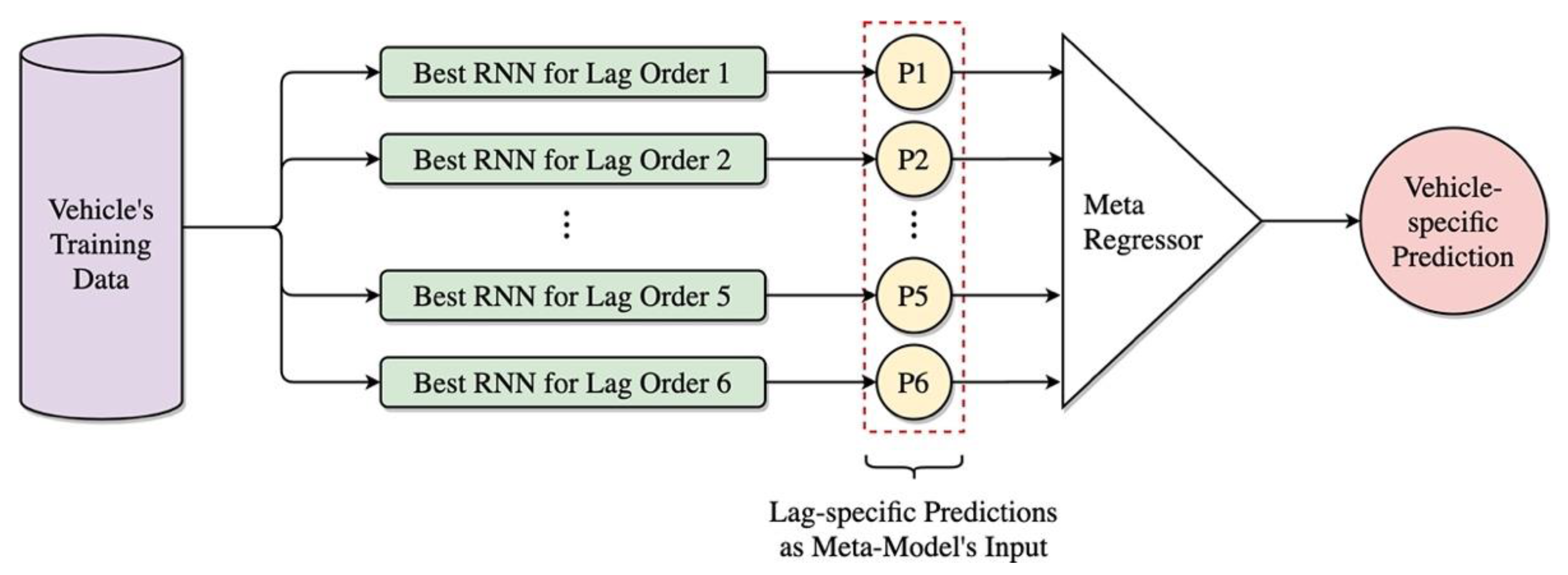
3.4. Primary Forecast Combination for Lag-Specific RNNs

The diversity of lag sources makes the true order of lag completely unknown and possibly dynamic. To deal with this uncertainty, we performed a grid search and trained RNN models for all the vehicle-dependent pairs with different cell structures, architecture depth (stacking), and lag orders ranging from 1 to 10 (the dependents are the FCR and ERs). The upper bound for the lag-order range was selected based on an engineering judgment and the notion that 10 s is long enough for dissipation of temporally distributed effects in vehicles’ physical operation. Figure 5 visually represents the average of normalized Root Mean Squared Error (RMSE) for the trained models. Note that the color in each cell reflects the average modeling score (ranging from 0 to 1) for the whole fleet under study, not a subset of vehicles.
The best results (highlighted with dashed yellow frames) were obtained for a range of lag orders from 1 to an average of 6. Considering the proven capability of RNNs in capturing serially-correlated and lagged effects, 6 s would be used as the maximum extent of lagged effects for the rest of the modeling procedure. This finding is consistent with our observation when speed and fuel/emissions curves were overlayed in our previous studies [66].
The results of RNN modeling for lag orders of 1 and 6 for a randomly selected time-window for three of the vehicles under study are presented in Figure 6.
The prediction curves clearly show that in terms of accuracy, L1 and L6 models compete with each other at different ranges. The RNNs with lower lag orders predict the extremes and sudden peaks/valleys much better (see regions highlighted in magenta), while those with higher lag orders perform better at ranges with smaller/no variations (see regions highlighted in yellow). The observation brings the idea that combining forecasts conducted by RNN models of different lag orders might lead to a single but more accurate model.
As the next step, forecast combination techniques are utilized to combine predictions of RNN models trained for each vehicle-dependent pair for each of the 6 lag orders (we call them lag-specific models). Taking this approach, we wish to come up with a Metamodel (or Meta-Regressor) for each vehicle-dependent pair expected to perform at least as good as the best lag-specific component model, if not outperforming it. The resulting metamodels will have the capability of dynamically weighting the output of lag-specific sub-models depending on the prevailing state of the vehicle operation at different time slots.
The primary metamodels will be used later for building higher-level ensembles for the categories of vehicles. Note that the modeling approach taken here is inspired by the Stacking method in the EL paradigm, where the component models are trained based on a complete dataset, and then their outputs are used as input variables to train an ensemble function (shown in Figure 7).
The performance of eight widely used EL algorithms (as the Meta-Regressors) is evaluated here. The best algorithm-setting combination was then selected for each vehicle. The algorithms and the corresponding major settings are described in Table 3.
For EL modeling at this stage, a similar 70–30% train-test splitting strategy and a five-fold cross validation is deployed. The results of the vehicle-specific forecast combination are visually presented and statistically discussed later in Section 4.

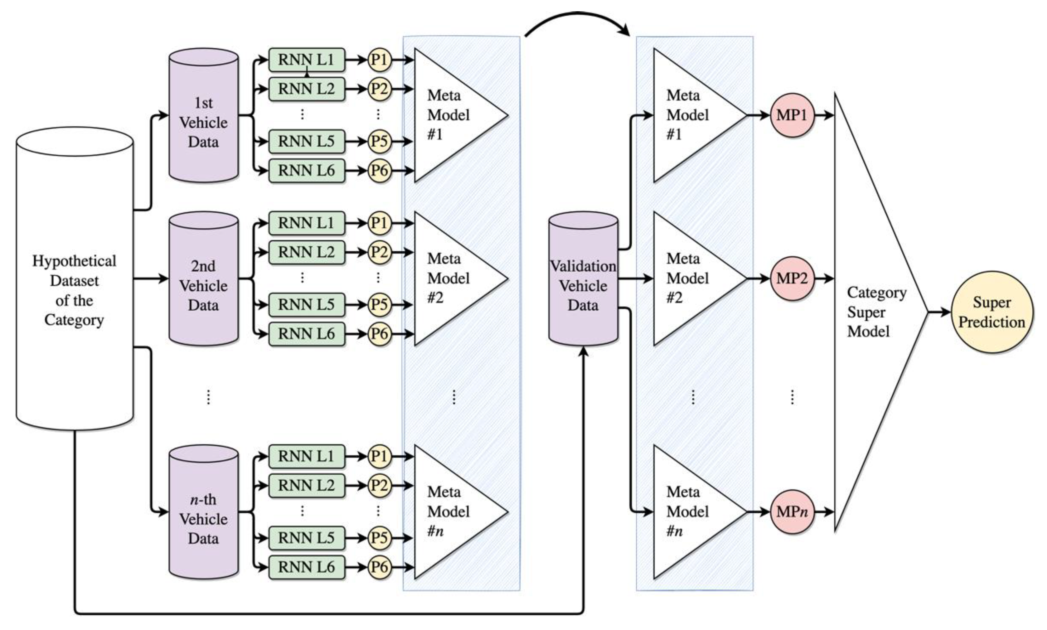
3.5. Category-Specific Ensemble Modeling

Vehicle-specific modeling is naturally susceptible to bias; hence, generalizing such models to other vehicles could always be criticized. Critiques could question how a model trained on a particular vehicle’s dataset is guaranteed to work as good for other vehicles which have different characteristics. Even vehicles from the same class (i.e., compact SUVs) come with various technical specifications that affect their pattern of fuel consumption and emissions generation. As an answer to this concern, higher level metamodels for categories (we call them, Supermodels) are trained through an extra layer of forecast combination on top of the vehicle-specific metamodels. Categorization of the vehicles could be done based on their general attributes such as vehicle class, weight, age, transmission technology, engine type, etc. However, we need to make a heavy assumption that all the vehicles in a category possess common attributes affecting their operation, which result in similar fuel consumption and emission generation patterns.
The data corresponding to each vehicle are assumed to be a subset of a larger hypothetical homogenous dataset dedicated to the category. Nevertheless, we cannot clearly say which common attributes lead to categories with such homogenized members. The categorization criteria can be ranked only after comparing the modeling scores of the category-specific supermodels. Figure 8 shows the comprehensive architecture of our two-stage EL approach for generalizing the basic RNN models to category-specific supermodels.
Because the vehicle-specific metamodels are trained for each vehicle’s dataset separately, the predictions regarding their test input data will not be valid for our second-level forecast combination. To deal with this issue and to avoid violating our heavy assumption regarding the homogeneity of category members, we take a Leave-One-Out Cross Validation (LOOCV) approach. After categorizing the vehicles based on the desired criterion, in every step of the cross validation, the training is conducted on n-1 vehicles out of n members of each category. Hence, during each training iteration, the model does not see the data regarding the nth vehicle at all. Each of the category members would play the role of left-out-vehicle once. As a result, the out-of-sample validation is repeated n times and the average of the validation scores is finally used for evaluating the prediction power of the supermodel.
The same set of EL algorithms and settings described in Table 3 are assessed for developing category-specific models. Vehicles are categorized based on six criteria of age, class, engine type, engine-size, transmission type, and weight (sum of curb weight and live/dead payload). RMSE is used in all three lag-, vehicle-, and category-specific modeling steps as the evaluation metric. Results of EL modeling attempts are visually presented and discussed in Section 4.

4. Results and Discussion

In this section, the results of all modeling steps taken in this study are discussed in the order of occurrence. Note that RMSE is the main metric used for evaluation of models’ prediction power; especially, when assessing the improvement of metamodels compared to lag-specific RNNs and the supermodels compared to metamodels. Also, R-squared is used wherever the predictions of our proposed mixed time-series and ensemble model are compared to benchmark models or only to the ground-truth (true observations).

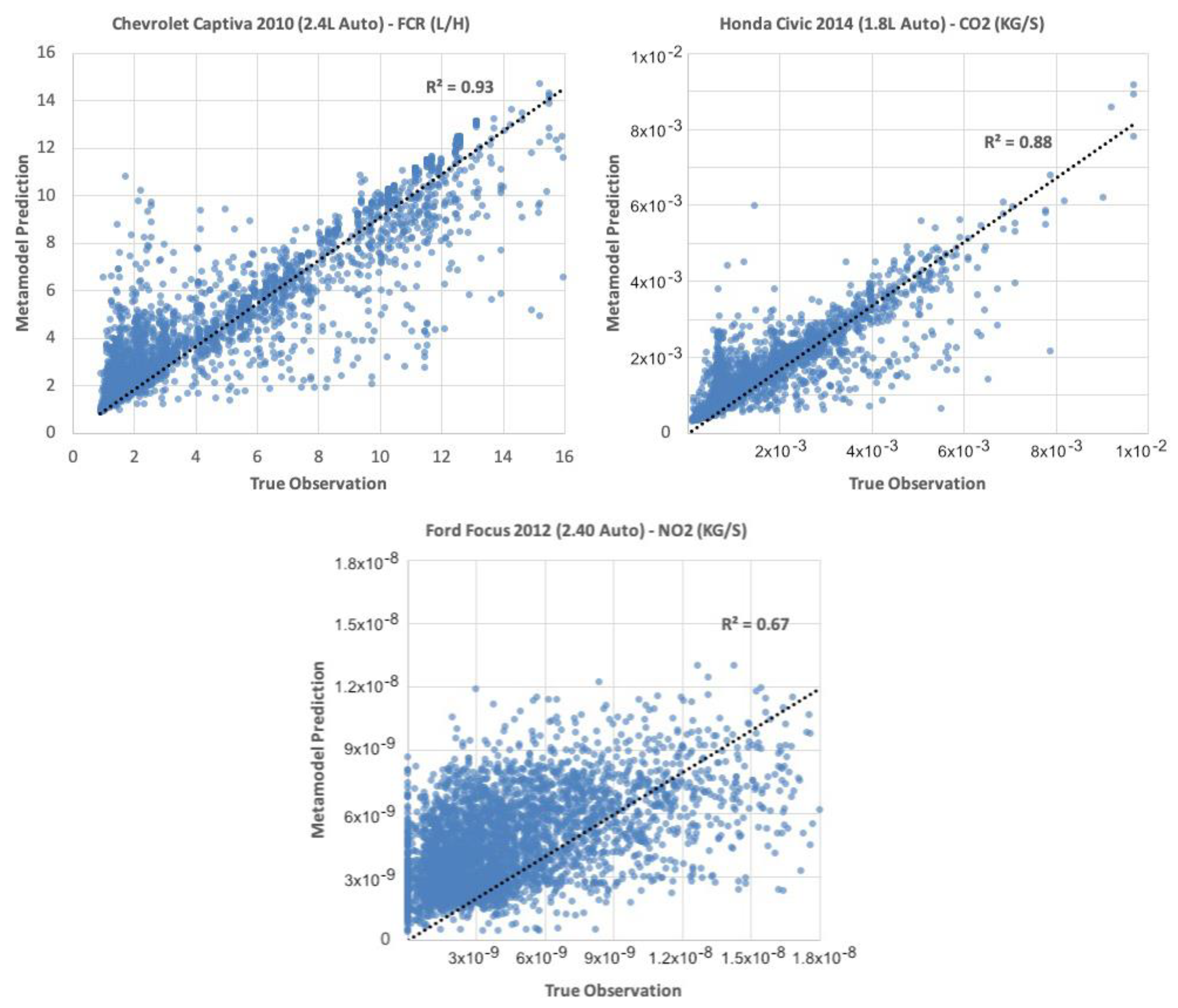
4.1. Metamodel Development Results

LSTM worked the best for about 75% of the vehicle, dependent, and lag-order combinations. Moreover, except for NO, having more than one layer of RNN (2 or 3) led to improved RMSE scores. As the level of NO emissions has low volatility, less-complex modeling architectures predict its rate acceptably.
The exceptional power of forecast combination algorithms was revealed during our metamodel development stage. In total, we developed 103 vehicle-specific metamodels including 35 for fuel rate in addition to 68 for emission rates (4 emission models for each of the 17 vehicles under study that we performed tailpipe measurements on them, all in Montreal). In 93 out of 103 metamodels, notable improvements in RMSE scores (up to 28% and on average 4%) was observed compared to that of the best lag-specific component models. Nevertheless, it is not guaranteed that the ensembles always perform better than the component models. It highly depends on the type of ensemble estimator as well as the level of the weakness of the component models.
In Figure 9, each bar shows the percentage of vehicles for which a particular ensemble estimator has led to the best meta-modeling RMSE score (the percentages in each of the 5 subsections, corresponding to the dependent-variable types, sum up to 100%). Also note that the horizontal axis shows the absolute number of vehicles-specific metamodels and the percentages are shown only next to the bars. Obviously, the random forest algorithm was the superior ensemble technique for FCR- and CO2-rate meta-modeling, whereas the much simpler method of Linear Regression led to the best results for NO2, NO, and PM rates.
Two conclusions could be drawn in this regard. First, minor differences exist between the predictions of different lag-specific models (as inputs of the EL models) for the FCR and CO2 rates. Hence, only more sophisticated EL algorithms could extract underlying nonlinear dependencies and achieve considerable improvements. It is noteworthy that the 28%, 23%, and 16% improvement records in RMSE, when comparing the metamodel score with the score of the best component model, are all dedicated to FCR and CO2 rate metamodels (an average of 6% improvement was achieved in this group of metamodels). Such high improvements confirm the existence of higher-level nonlinear dependencies that the lag-specific RNNs were incapable of capturing them alone.
Second, the lag-specific RNN predictions for NO, NO2, and PM are varied enough and as inputs to metamodels, they possess such linear correlations with the dependent which allows forecast combinations such as simple unregularized linear regression algorithm to work efficiently and even lead to score improvements. The average improvement for the discussed emissions is equal to 2%. The lower average improvement in RMSE score compared to FCR and CO2 metamodels could be due to the dominant effect of one lag-specific component model on the metamodel performance. A possible interpretation is that for NOx and PM emissions, the existence of a relatively constant lag order is feasible, while for fuel and CO2, distributively lagged effects exist.
Predictions of metamodels regarding three sample vehicle-dependent pairs are presented in Figure 10. The EL algorithms show undeniable effectiveness for FCR and CO2 rate.
It is interesting how the EL algorithms have corrected some of the wrong local trends predicted by lag-specific RNN models (see regions highlighted in yellow). Moreover, metamodels have compensated component models’ weakness in predicting sudden spikes (see regions highlighted in magenta). Even for the NOx and PM, despite the higher level of prediction error, the metamodel outperforms the lag-specific component models. In Figure 11, the true observations are compared to the metamodel predictions for all data points corresponding to the same three vehicles-dependent pairs presented in Figure 10.

4.2. Validating Metamodels

Independent from the relative improvements achieved by the metamodels (compared to their component models), their absolute accuracy could be a matter of concern. We take three steps to validate our models and prove their strength compared to the models of the same class.
First, meta-regressors similar to those used for developing vehicle-specific metamodels (random forest for FCR and CO2 and linear regression for NOx and PM) are directly applied on data (by skipping the RNN modeling step) and the modeling scores are compared to that of the metamodels. By this comparison, we look to emphasize the impact of mixed modeling methodology (mixture of EL and RNN techniques) in achieving outstanding RMSE scores and to prove that use of meta-regressors alone would not be enough to achieve such scores. As shown in Figure 12, the metamodels outperformed the direct models for all vehicle-dependent pairs with an average margin of 13% (and a maximum of 38%) regarding the RMSE score. Only for 8 out of 103 vehicle-dependent pairs (most of which corresponding to NO), the direct model has scored a lower RMSE value. Such few outliers were expected as our NO-metamodels were already among the weakest compared to the fuel and other emissions.
In the second validation step, the predictions of the FCR metamodels are compared to that of VT-CPFM [5,25], one of the most sophisticated power-based instantaneous fuel models proposed in the literature. The VT-CPFM utilizes Vehicle Specific Power (VSP) formula [67] to estimate the instantaneous power demand with detailed consideration of the impact of aerodynamic drag, rolling resistance, road grade, vehicle’s drive-line efficiency, and even transmission system characteristics. The estimated power is then used as a proxy explanatory variable to calibrate a piecewise polynomial function to estimate FCR. The out-of-sample test scores (R-squared) of the models are presented and compared side-by-side in Table 4.
Figure 13 visually compares true FCR with predictions of metamodel the benchmark model the 3 of the test vehicles (a random time-window is shown).
Obviously, our RNN-based metamodels have made more accurate predictions, despite all the parametric adjustments applied on VT-CPFM model for specific characteristics of the vehicle and fuel type.
For the final validation step, we assess the performance of our metamodels at different temporal resolutions. Our mixed EL and RNN methodology is relatively complex compared to simpler time-series modeling techniques such as Auto-Regressive Integrated Moving Average (ARIMA). Also, higher resolution models normally have more specific use cases (in our case, we target eco-driving purposes). So, one might question the benefit of having precise and complex fuel and emission models at 1-sec temporal scale when lower-resolution (for instance, 5-s or 10-s scale) but less-sophisticated models might be enough for the needs of analysis. To this end, ARIMA model is trained at three scales of 1, 5, and 10 s (average values for variables and dependent are used for 5- and 10-s intervals) for three vehicles. The modeling R-squared scores are then compared to that of aggregated outputs of our high-resolutions metamodels (Table 5). Note that in addition to ARIMA predictions, the average of the second-by-second metamodel predictions and true observations for 5- and 10-s time slots are used for calculating R-squared score at aggregate levels.
Our metamodels not only outperformed the simpler time-series ARIMA architecture at 1-s scale but also, they kept their superiority with almost a similar margin at 5-s and 10-s scales. Hence, developing accurate high-resolution models for fuel and emission estimation contributes significantly to situations where lower-resolution predictions are desired as well.

4.3. Supermodel Development Results

Regarding the category-specific supermodels, an average RMSE score improvement of 6% (with records up to 32%) compared to the best component metamodels is achieved. Although the same set of EL algorithms is used for developing the supermodels, relatively higher score improvements have occurred. The diversity of the datasets corresponding to different category members, is one of the important root causes of this notable difference, notwithstanding the heavy assumption we made about considering category member’s datasets homogenous subsets of a hypothetical larger dataset.
Taking a look at the RMSE scores of the ensemble category-specific supermodels, all positive score improvements with rare zero values are achieved. This supports the idea that EL algorithms could work as a unifying medium for developing higher-level (aggregate) microscale fuel and emission models. Transmission Type seems to be the most efficient aggregation measure for FCR supermodels. The transmission system directly deals with the quality of power transmission from the engine to the wheels and has a significant impact on the efficiency of the combustion process. Hence, its importance regarding fuel consumption and CO2 generation is expectable. However, this criterion does not seem appropriate for NO and PM emissions where limited improvements is achieved.
Modifying the categorization thresholds or combining some of the categories could lead to more homogenous improvements among categories. For instance, the low RMSE score improvement achieved for the Compact SUV class (3% compared to an average of 13% for other classes) for FCR supermodels brings the idea of merging this class with another one.
The Age Range criterion seems to work best for the PM rate (with a record of 21% RMSE score improvement for age range between 3 and 5). The aging of the vehicle leads to physical degradation of the engine and adds to the inefficiencies of the powertrain. Moreover, in an aged vehicle, usually the catalytic converter and the particulate filters lose their effectiveness resulting in higher PM rates.
Although small, there were positive improvements for all NO-related supermodels. As mentioned earlier, the low volatility of NO-rate observations makes predictions of much simpler nonlinear modeling algorithms (even single-stage and without EL) acceptable enough. Such weak results (compared to other emissions and FCR), could be linked to the sensor measurement errors as well. Although the state-of-the-technology PEMS units deployed in this study provides unbeatable accuracies, as NOx emission rates are generally so low in gasoline-engine vehicles, even minor sensor errors affect the readings considerably.
Figure 14 shows that even for the supermodels, sophisticated algorithms (Gradient Boosting as well as Random Forest) outperform others for the majority of criteria/categories for FCR and CO2 rate, while similar to the metamodels, Linear and Ridge Regressions shoulder the forecast combination burden of NOx and PM supermodels better.
Gradient Boosting and Random Forest algorithms both use Decision Trees at their core and combine their forecasts to achieve better results, however, the former builds trees one at a time, where each new tree helps to correct errors made by the previously trained tree. Their difference could be better explained using the concept of bias and variance in the ML paradigm. Boosting is based on weak learners which have high bias and low variance (like the vehicle-specific metamodels in each category) and it reduces errors mainly by reducing bias. On the other hand, Random Forest uses fully grown decision trees with low bias and high variance (similar to lag-specific RNNs). It tackles the error reduction task by reducing variance. This explanation clarifies why Gradient Boosting and Random Forest algorithms have been the dominant best estimators for supermodel and metamodel development, respectively.
Finally, in Figure 15, sample time-windows are randomly selected for 3 category-dependent pairs to visually evaluate the performance of trained supermodels.
Figure 16 depicts the impressive accuracy of the proposed two-stage EL approach, where for FCR and CO2 rates, R-squared scores of 0.95 and 0.88 are achieved, respectively. The method has made acceptable predictions for NO2 as well, although it appears to be weak in capturing peaks. Nevertheless, as our categorization process still requires refinement, an R-squared score of 0.7 seems a satisfying score at this stage.

5. Conclusions and Future Work

In this study, we targeted the development of a methodology for estimating microscale fuel consumption and emission models deployable in smartphone-based eco-driving assistance services or in combination with the existing traffic microsimulation models. We first addressed the dynamicity of the lag order through mixed use of time-series and ensemble modeling. Then by using an additional layer of forecast combination on top of first-stage mixed models, we developed a robust methodology for generalizing models to categories of vehicles.
Our vehicle-specific metamodels showed improvement records of up to 28% concerning the RMSE score (with an average improvement of 4% among different vehicles and dependent types) compared to that of the best lag-specific component models. Moreover, our generalized supermodels even outperformed the component metamodels by a margin of up to 32% regarding RMSE score (with an average of 6% among different criteria/categories). Our proposed methodology opens avenues to use of machine learning techniques for rapid development of light, generalized, and localized microscale fuel and emission models calibrated using field data.
A few aspects could be addressed in future works. Although large compared to many other studies, the test-fleet size and its diversity could be increased to hundreds of vehicles and many planned experiments on particular vehicles could be run. In the light of a such large and diverse dataset, the impacts of unseen factors like vehicle weight, number of passengers, use of auxiliary components, weather conditions, etc. could be included in the models as well. Furthermore, due to technical limitations of the PEMS units, we disregarded cold-start operation and the tire-/brake-wear emissions which could be exclusively studied using appropriate equipment.

Author Contributions

Conceptualization, E.M.; Methodology, E.M. and L.M.-M.; Software, E.M.; Validation, L.M.-M.; Formal Analysis, E.M.; Investigation, E.M. and L.M.-M.; Data Curation, E.M.; Writing—Original draft preparation, E.M.; Visualization, E.M.; Supervision, L.M.-M.; Writing—Reviewing and Editing, L.M.-M. All authors have read and agreed to the published version of the manuscript.

Funding

This research received no external funding.

Institutional Review Board Statement

Not applicable.

Informed Consent Statement

Not applicable.

Data Availability Statement

The data presented in this study are available on request from the corresponding author. The data are not publicly available due to being owned by McGill University (Department of Civil Engineering).

Conflicts of Interest

The authors declare no conflict of interest.

References

  1. Bifulco, G.N.; Galante, F.; Pariota, L.; Spena, M.R. A Linear Model for the Estimation of Fuel Consumption and the Impact Evaluation of Advanced Driving Assistance Systems. Sustainability 2015, 7, 14326–14343. [Google Scholar] [CrossRef] [Green Version]
  2. Çapraz, A.G.; Özel, P.; Sevkli, M.; Beyca Ömer, F. Fuel Consumption Models Applied to Automobiles Using Real-time Data: A Comparison of Statistical Models. Procedia Comput. Sci. 2016, 83, 774–781. [Google Scholar] [CrossRef] [Green Version]
  3. Frey, H.C.; Zhang, K.; Rouphail, N. Vehicle-Specific Emissions Modeling Based upon on-Road Measurements. Environ. Sci. Technol. 2010, 44, 3594–3600. [Google Scholar] [CrossRef] [PubMed]
  4. Nie, Y.; Li, Q. An eco-routing model considering microscopic vehicle operating conditions. Transp. Res. Part B Methodol. 2013, 55, 154–170. [Google Scholar] [CrossRef]
  5. Rakha, H.A.; Ahn, K.; Moran, K.; Saerens, B.; Van Den Bulck, E. Virginia Tech Comprehensive Power-Based Fuel Consumption Model: Model development and testing. Transp. Res. Part D Transp. Environ. 2011, 16, 492–503. [Google Scholar] [CrossRef]
  6. Saerens, B.; Rakha, H.; Ahn, K.; Bulck, E.V.D. Assessment of Alternative Polynomial Fuel Consumption Models for Use in Intelligent Transportation Systems Applications. J. Intell. Transp. Syst. 2012, 17, 294–303. [Google Scholar] [CrossRef]
  7. Zhou, Q.; Gullitti, A.; Xiao, J.; Huang, Y. Neural network-based modeling and optimization for effective vehicle emission testing and engine calibration. Chem. Eng. Commun. 2008, 195, 706–720. [Google Scholar] [CrossRef]
  8. Koupal, J.; Cumberworth, M.; Michaels, H.; Beardsley, M.; Brzezinski, D. Design and Implementation of MOVES: EPA’s New Generation Mobile Source Emission Model. Int. Emiss. Invent. Conf. 2003, 1001, 105. [Google Scholar]
  9. Scora, G.; Barth, M. Comprehensive Modal Emissions Model (CMEM), Version 3.01 User’s Guide; University of California: Riverside, CA, USA, 2006; p. 1070. [Google Scholar]
  10. Guensler, R.; Liu, H.; Xu, X.; Xu, Y.; Rodgers, M.O. MOVES-Matrix: Setup, implementation, and application. In Proceedings of the 95th Annual Meeting of the Transportation Research Board, Washington, DC, USA, 10–14 January 2016. [Google Scholar]
  11. Ntziachristos, L.; Gkatzoflias, D.; Kouridis, C.; Samaras, Z. COPERT: A European Road Transport Emission Inventory Model. In Information Technologies in Environmental Engineering; Springer: Berlin/Heidelberg, Germany, 2009; pp. 491–504. [Google Scholar]
  12. Stockholm Environment Institute. Low Emissions Analysis Platform (LEAP). 2020. Available online: https://leap.sei.org/default.asp?action=home (accessed on 22 September 2021).
  13. Moradi, E.; Miranda-Moreno, L. On-road vs. Software-based Measurements: On Validity of Fuel, CO2, NOx, and PM Predictions by US EPA’s MOVES. In Proceedings of the Transportation Research Board 100th Annual Meeting, Washington, DC, USA, 9–13 January 2021. [Google Scholar]
  14. Duarte, G.; Gonçalves, G.; Baptista, P.; Farias, T. Establishing bonds between vehicle certification data and real-world vehicle fuel consumption—A Vehicle Specific Power approach. Energy Convers. Manag. 2015, 92, 251–265. [Google Scholar] [CrossRef]
  15. Kayes, D.; Hochgreb, S. Mechanisms of Particulate Matter Formation in Spark-Ignition Engines. 3. Model of PM Formation. Environ. Sci. Technol. 1999, 33, 3978–3992. [Google Scholar] [CrossRef]
  16. Zhai, H.; Frey, H.C.; Rouphail, N. A Vehicle-Specific Power Approach to Speed- and Facility-Specific Emissions Estimates for Diesel Transit Buses. Environ. Sci. Technol. 2008, 42, 7985–7991. [Google Scholar] [CrossRef] [PubMed]
  17. Moradi, E.; Miranda-Moreno, L. Vehicular fuel consumption estimation using real-world measures through cascaded machine learning modeling. Transp. Res. Part D Transp. Environ. 2020, 88, 102576. [Google Scholar] [CrossRef]
  18. Arrègle, J.; López, J.J.; Guardiola, C.; Monin, C. Sensitivity Study of a NOx Estimation Model for On-Board Applications; SAE International: Washington, DC, USA, 2008. [Google Scholar]
  19. Demesoukas, S. 0D/1D Combustion Modeling for the Combustion Systems Optimization of Spark Ignition Engines; Université d′Orléans: Montpellier, France, 2015. [Google Scholar]
  20. Payri, F.; Arrègle, J.; López, J.J.; Mocholí, E. Diesel NOx Modeling with a Reduction Mechanism for the Initial NOx Coming from EGR or Re-Entrained Burned Gases; SAE International: Warrendale, PA, USA, 2008. [Google Scholar]
  21. Saerens, B.; Diehl, M.; Bulck, E.V.D. Optimal Control Using Pontryagin’s Maximum Principle and Dynamic Programming. In Automotive Model Predictive Control; Springer: Berlin/Heidelberg, Germany, 2010; pp. 119–138. [Google Scholar] [CrossRef]
  22. Tauzia, X.; Karaky, H.; Maiboom, A. Evaluation of a semi-physical model to predict NOx and soot emissions of a CI automotive engine under warm-up like conditions. Appl. Therm. Eng. 2018, 137, 521–531. [Google Scholar] [CrossRef]
  23. Anetor, L.; Odetunde, C.; Osakue, E.E. Computational Analysis of the Extended Zeldovich Mechanism. Arab. J. Sci. Eng. 2014, 39, 8287–8305. [Google Scholar] [CrossRef]
  24. Blauwens, J.; Smets, B.; Peeters, J. Mechanism of “prompt” no formation in hydrocarbon flames. Symp. Combust. 1977, 16, 1055–1064. [Google Scholar] [CrossRef]
  25. Rakha, H.A.; Ahn, K.; Faris, W.; Moran, K.S. Simple Vehicle Powertrain Model for Modeling Intelligent Vehicle Applications. IEEE Trans. Intell. Transp. Syst. 2012, 13, 770–780. [Google Scholar] [CrossRef]
  26. Du, Y.; Wu, J.; Yang, S.; Zhou, L. Predicting vehicle fuel consumption patterns using floating vehicle data. J. Environ. Sci. 2017, 59, 24–29. [Google Scholar] [CrossRef]
  27. Kim, D.; Lee, J. Application of Neural Network Model to Vehicle Emissions. Int. J. Urban Sci. 2010, 14, 264–275. [Google Scholar] [CrossRef]
  28. Li, Q.; Qiao, F.; Yu, L. A Machine Learning Approach for Light-Duty Vehicle Idling Emission Estimation Based on Real Driving and Environmental Information. Environ. Pollut. Clim. Change 2017, 1, 106. [Google Scholar] [CrossRef]
  29. Wu, J.-D.; Liu, J.-C. A forecasting system for car fuel consumption using a radial basis function neural network. Expert Syst. Appl. 2012, 39, 1883–1888. [Google Scholar] [CrossRef]
  30. Ajtay, D.; Weilenmann, M. Static and dynamic instantaneous emission modelling. Int. J. Environ. Pollut. 2004, 22, 226–239. [Google Scholar] [CrossRef]
  31. Jaikumar, R.; Nagendra, S.S.; Sivanandan, R. Modeling of real time exhaust emissions of passenger cars under heterogeneous traffic conditions. Atmos. Pollut. Res. 2017, 8, 80–88. [Google Scholar] [CrossRef]
  32. Adhikari, R. A neural network based linear ensemble framework for time series forecasting. Neurocomputing 2015, 157, 231–242. [Google Scholar] [CrossRef]
  33. Bianchi, F.M.; Maiorino, E.; Kampffmeyer, M.C.; Rizzi, A.; Jenssen, R. An overview and comparative analysis of recurrent neural networks for short term load forecasting. arXiv 2017, arXiv:1705.04378. [Google Scholar]
  34. Kourentzes, N.; Barrow, D.K.; Crone, S.F. Neural network ensemble operators for time series forecasting. Expert Syst. Appl. 2014, 41, 4235–4244. [Google Scholar] [CrossRef] [Green Version]
  35. Kang, D.; Lv, Y.; Chen, Y.-Y. Short-term traffic flow prediction with LSTM recurrent neural network. In Proceedings of the 2017 IEEE 20th International Conference on Intelligent Transportation Systems (ITSC), Yokohama, Japan, 16–19 October 2017; IEEE Press: Piscataway, NJ, USA, 2017; pp. 1–6. [Google Scholar]
  36. Lee, Y.-J.; Min, O. Long Short-Term Memory Recurrent Neural Network for Urban Traffic Prediction: A Case Study of Seoul. In Proceedings of the 2018 21st International Conference on Intelligent Transportation Systems (ITSC), Maui, HI, USA, 4–7 November 2018; IEEE Press: Piscataway, NJ, USA, 2018; pp. 1279–1284. [Google Scholar]
  37. Han, S.; Zhang, F.; Xi, J.; Ren, Y.; Xu, S. Short-term vehicle speed prediction based on Convolutional bi-directional LSTM networks. In Proceedings of the 2019 IEEE Intelligent Transportation Systems Conference (ITSC), Auckland, New Zealand, 27–30 October 2019; pp. 4055–4060. [Google Scholar]
  38. Wang, H.; Luo, H.; Zhao, F.; Qin, Y.; Zhao, Z.; Chen, Y. Detecting transportation modes with low-power-consumption sensors using recurrent neural network. In Proceedings of the 2018 IEEE SmartWorld, Ubiquitous Intelligence & Computing, Advanced & Trusted Computing, Scalable Computing & Communications, Cloud & Big Data Computing, Internet of People and Smart City Innovation (SmartWorld/SCALCOM/UIC/ATC/CBDCom/IOP/SCI), Guangzhou, China, 8–12 October 2018; pp. 1098–1105. [Google Scholar]
  39. Luo, D.; Lu, J.; Guo, G. Road Anomaly Detection Through Deep Learning Approaches. IEEE Access 2020, 8, 117390–117404. [Google Scholar] [CrossRef]
  40. Bai, M.; Lin, Y.; Ma, M.; Wang, P. Travel-Time Prediction Methods: A Review. In Proceedings of the 3rd International Conference on Smart Computing and Communication, Tokyo, Japan, 10–12 December 2018; pp. 67–77. [Google Scholar]
  41. Duan, Y.; Yisheng, L.V.; Wang, F.-Y. Travel time prediction with LSTM neural network. In Proceedings of the 2016 IEEE 19th International Conference on Intelligent Transportation Systems (ITSC), Rio de Janeiro, Brazil, 1–4 November 2016; IEEE Press: Piscataway, NJ, USA, 2016; pp. 1053–1058. [Google Scholar]
  42. Jakteerangkool, C.; Muangsin, V. Short-Term Travel Time Prediction from GPS Trace Data using Re-current Neural Networks. In Proceedings of the 2020 Asia Conference on Computers and Communications (ACCC), Singapore, 4–6 December 2020; pp. 62–66. [Google Scholar]
  43. Lee, E.H.; Kho, S.-Y.; Kim, D.-K.; Cho, S.-H. Travel time prediction using gated recurrent unit and spatio-temporal algorithm. Proc. Inst. Civ. Eng.-Munic. Eng. 2021, 174, 88–96. [Google Scholar] [CrossRef]
  44. Liu, Y.; Wang, Y.; Yang, X.; Zhang, L. Short-term travel time prediction by deep learning: A comparison of different LSTM-DNN models. In Proceedings of the 2017 IEEE 20th International Conference on Intelligent Transportation Systems (ITSC), Yokohama, Japan, 16–19 October 2017; Available online: https://ieeexplore.ieee.org/document/8317886 (accessed on 15 September 2021).
  45. Ran, X.; Shan, Z.; Fang, Y.; Lin, C. An LSTM-based method with attention mechanism for travel time prediction. Sensors 2019, 19, 861. [Google Scholar] [CrossRef] [Green Version]
  46. Zhao, J.; Gao, Y.; Qu, Y.; Yin, H.; Liu, Y.; Sun, H. Travel Time Prediction: Based on Gated Recurrent Unit Method and Data Fusion. IEEE Access 2018, 6, 70463–70472. [Google Scholar] [CrossRef]
  47. Kanarachos, S.; Mathew, J.; Fitzpatrick, M.E. Instantaneous vehicle fuel consumption estimation using smartphones and recurrent neural networks. Expert Syst. Appl. 2019, 120, 436–447. [Google Scholar] [CrossRef]
  48. Jose, V.R.; Winkler, R.L. Simple robust averages of forecasts: Some empirical results. Int. J. Forecast. 2008, 24, 163–169. [Google Scholar] [CrossRef]
  49. Wu, M. Trimmed and Winsorized Estimators; Michigan State University: East Lansing, MI, USA, 2006. [Google Scholar]
  50. Chan, L.-W. Weighted least square ensemble networks. In Proceedings of the IJCNN’99—International Joint Conference on Neural Networks, Washington, DC, USA, 10–16 July 1999. [Google Scholar]
  51. Ferreira, W.G.; Serpa, A.L. Ensemble of metamodels: The augmented least squares approach. Struct. Multidiscip. Optim. 2016, 53, 1019–1046. [Google Scholar] [CrossRef]
  52. Hansen, B.E. Least-squares forecast averaging. J. Econ. 2008, 146, 342–350. [Google Scholar] [CrossRef] [Green Version]
  53. Ren, Y.; Zhang, L.; Suganthan, P. Ensemble Classification and Regression-Recent Developments, Applications and Future Directions. IEEE Comput. Intell. Mag. 2016, 11, 41–53. [Google Scholar] [CrossRef]
  54. Sagi, O.; Rokach, L. Ensemble learning: A survey. WILEY Interdiscip. Rev. Data Min. Knowl. Discov. 2018, 8, e1249. [Google Scholar] [CrossRef]
  55. Agamennoni, G.; Nieto, J.I.; Nebot, E. An outlier-robust Kalman filter. In Proceedings of the 2011 IEEE International Conference on Robotics and Automation, Shanghai, China, 9–13 May 2011; pp. 1551–1558. [Google Scholar]
  56. Press, W.; Teukolsky, S.A. Savitzky-Golay Smoothing Filters. Comput. Phys. 1990, 4, 669. [Google Scholar] [CrossRef]
  57. Lambda and Engine Performance. Available online: https://x-engineer.org/automotive-engineering/internal-combustion-engines/performance/air-fuel-ratio-lambda-engine-performance/ (accessed on 18 October 2021).
  58. Che, Z.; Purushotham, S.; Cho, K.; Sontag, D.; Liu, Y. Recurrent Neural Networks for Multivariate Time Series with Missing Values. Sci. Rep. 2018, 8, 6085. [Google Scholar] [CrossRef] [Green Version]
  59. Gers, F.A.; Schmidhuber, J.; Cummins, F. Learning to Forget: Continual Prediction with LSTM. Neural Comput. 2000, 12, 2451–2471. [Google Scholar] [CrossRef] [PubMed]
  60. Hochreiter, S.; Schmidhuber, J. Long short-term memory. Neural Comput. 1997, 9, 1735–1780. [Google Scholar] [CrossRef]
  61. Lipton, Z.C.; Berkowitz, J.; Elkan, C. A Critical Review of Recurrent Neural Networks for Sequence Learning. arXiv 2015, arXiv:1506.00019. [Google Scholar]
  62. Alcan, G.; Yilmaz, E.; Unel, M.; Aran, V.; Yilmaz, M.; Gurel, C.; Koprubasi, K. Estimating Soot Emission in Diesel Engines Using Gated Recurrent Unit Networks. IFAC-PapersOnLine 2019, 52, 544–549. [Google Scholar] [CrossRef]
  63. Chung, J.; Gulcehre, C.; Cho, K.; Bengio, Y. Gated feedback recurrent neural networks. In Proceedings of the 32nd International Conference on Machine Learning, Lille, France, 6–11 July 2015. [Google Scholar]
  64. Abadi, M.; Barham, P.; Chen, J.; Chen, Z.; Davis, A.; Dean, J.; Devin, M.; Ghemawat, S.; Irving, G.; Isard, M.; et al. TensorFlow: A system for large-scale machine learning. In Proceedings of the 12th USENIX Symposium on Operating Systems Design and Implementation, Savannah, GA, USA, 2–4 November 2016. [Google Scholar]
  65. Pedregosa, F.; Varoquaux, G.; Gramfort, A.; Michel, V.; Thirion, B.; Grisel, O.; Blondel, M.; Prettenhofer, P.; Weiss, R.; Dubourg, V. Scikit-learn: Machine learning in Python. J. Mach. Learn. Res. 2011, 12, 2825–2830. [Google Scholar]
  66. Behan, M.; Moradi, E.; Miranda-Moreno, L. A Comparative Analysis of the Vehicular Emissions Generated as a Results of Different Intersection Controls. In Proceedings of the Transportation Research Board 99th Annual Meeting, Washington, DC, USA, 12–16 January 2020. [Google Scholar]
  67. Jimenez-Palacios, J.L. Understanding and Quantifying Motor Vehicle Emissions with Vehicle Specific Power and TILDAS Remote Sensing. Ph.D. Thesis, Massachusetts Institute of Technology, Cambridge, MA, USA, 1998. [Google Scholar]
Figure 1. Details of the OBD-II logger and the PEMS device installed on a test vehicle.
Sustainability 14 01900 g001
Figure 2. The aggregated trajectory of experiments in Montreal (left) and Bucaramanga (right) in form of a heatmap.
Sustainability 14 01900 g002
Figure 3. The data collection and preparation procedure.
Sustainability 14 01900 g003
Figure 4. The (a) Simple, (b) LSTM, and (c) GRU structures of RNN cells as well as a (d) stacked many-to-one RNN architecture with lag order of p (RNN cells shown in green color).
Sustainability 14 01900 g004
Figure 5. Average normalized RMSE scores considering different RNN settings for FCR (top), CO2 (middle), and PM (bottom).
Sustainability 14 01900 g005
Figure 6. RNN predictions for lag orders of 1 and 6 for FCR, NO2, and PM rates (corresponding to three sample vehicles).
Sustainability 14 01900 g006
Figure 7. A stacking ensemble learning architecture to develop vehicle-specific metamodels.
Sustainability 14 01900 g007
Figure 8. The two-stage EL approach for category-specific modeling (all the n vehicles as well as the validation vehicle correspond to one category).
Sustainability 14 01900 g008
Figure 9. Share of different ensemble estimators leading to best RMSE score when applied for different vehicles for modeling each of the dependent variables (FCR and ERs). Note that the horizontal axis shows the absolute number of vehicle-specific models.
Sustainability 14 01900 g009
Figure 10. Sample time-windows showing the prediction power of vehicle-specific metamodels in comparison with the lag-specific component models for three sample vehicle-dependent pairs.
Sustainability 14 01900 g010
Figure 11. A scatter-plot for comparing the true observation and metamodel predictions regarding the three vehicle-dependent pairs visualized in time-series format in Figure 10.
Sustainability 14 01900 g011
Figure 12. The percentage difference of the RMSE score between vehicle-specific metamodels and the direct models for all the vehicles under study.
Sustainability 14 01900 g012
Figure 13. Sample time-windows comparing the prediction power of the metamodel to true observations as well as predictions by the benchmark model (VT-CPFM).
Sustainability 14 01900 g013
Figure 14. Share of different ensemble estimators leading to best RMSE score when applied for different categories for modeling each of the dependent variables (FCR and ERs). Note that the horizontal axis shows the absolute number of category-specific models.
Sustainability 14 01900 g014
Figure 15. Random sample time-windows showing the prediction power of supermodels for 3 different category-dependent pairs.
Sustainability 14 01900 g015
Figure 16. Comparison between true observation and supermodel predictions for three selected category-dependent pairs.
Sustainability 14 01900 g016
Table 1. Field experiments’ summary.
AttributeCity
MontrealBucaramangaTehran
Total Trip Length (km)1804291255
Total Trip Time (Minutes)5224825444
Number of Test Vehicles2276
Table 2. Test fleet distribution based on different criteria.
CriterionCategoryCount
Vehicle SegmentsSUV8
Sedan19
Van1
Hatchback7
Engine TypesRegular31
Turbo-Charged4
Transmission TypesManual6
Automatic19
Dual-Clutch (Auto)2
CVT (Auto)8
Table 3. Details of EL algorithms evaluated for developing vehicle-specific meta-models.
AlgorithmSettings
AttributeValue
Linear RegressionFeature Scaling *Active
Ridge RegressionRegularization Strength α = {0.1, 1.0}
Support Vector Regression (SVR)KernelRadial Basis Function (RBF)
GammaScale
Epsilon0.1
Regularization ParameterC = {1.0, 10.0}
Decision TreeSplitting CriterionMean Squared Error (MSE)
Splitting Strategy at Nodes{Best, Random}
Maximum Tree DepthUnbounded
Gradient BoostingLoss FunctionLeast Squares Regression
Splitting CriterionMean Squared Error (MSE)
Learning Rate0.1
Number of Boosting Stages{10, 100}
AdaBoostBase EstimatorDecision Tree Regressor
Loss FunctionLinear
Learning Rate1.0
Number of Boosting Stages{10, 100}
Random ForestNumber of Trees{10, 100}
Splitting CriterionMean Squared Error (MSE)
Maximum Forest DepthUnbounded
Fully-Connected ANNNumber of Hidden Layers{1, 2}
Layer Size (No. of Neurons)100
Activation FunctionReLU
OptimizerAdam
Learning Rate0.001
Maximum No. of Iterations200
* Feature scaling in form of mean normalization is applied to data before evaluating each of the algorithms listed above.
Table 4. Side-by-side comparison of metamodel and benchmark model’s out-of-sample test scores.
VehicleModel Score (R-Squared)
MetamodelVT-CPFM
Hyundai Elantra GT 2019 (2.0 L Auto)0.720.57
Chevrolet Captiva 2010 (2.4 L Auto)0.860.26
Chevrolet Cruze 2011 (1.8 L Manual)0.770.52
Table 5. Comparison of ARIMA and metamodel R-squared scores at different temporal scales.
VehicleTemporal Scale/Model Type
1-s5-s10-s
ARIMAMetamodelARIMAMetamodelARIMAMetamodel
Hyundai Elantra GT 2019
(2.0 L Auto)
0.530.690.660.830.710.84
Chevrolet Captiva 2010
(2.4 L Auto)
0.110.860.250.920.230.94
Chevrolet Cruze 2011
(1.8 L Manual)
0.560.770.670.830.70.84
Publisher’s Note: MDPI stays neutral with regard to jurisdictional claims in published maps and institutional affiliations.

