Day-Ahead DSM-Integrated Hybrid-Power-Management-Incorporated CEED of Solar Thermal/Wind/Wave/BESS System Using HFPSO

Abstract

This paper presents a day-ahead demand-side management (DSM)-integrated hybrid power management algorithm (PMA) with an objective of combined economic and emission load dispatch (CEED) considering losses. The algorithm was tested on an IEEE 30-bus six-generator system consisting of solar thermal/wind/wave/battery energy storage systems (BESSs) considering real-time data of the Gujarat (19°07′ N, 72°51′ E) coastal region and diverse renewable energy (RES) and storage sources. A maiden attempt of utilizing hybrid firefly particle swarm optimization (HFPSO) to reduce thermal energy consumption and carbon emission was presented. Further, a novel attempt for a versatile renewable power management system was proposed based on a day-ahead pricing scheme to manage load demand and generation effectively. The PMA permits the users to bring down the general load demand and adjust the load curve during the peak time frame. The comparative performance of particle swarm optimization (PSO), firefly algorithm (FA), and HFPSO algorithms in solving the objective was presented. The HFPSO algorithm was found to be the best in terms of a fuel cost of 544.160 (USD/h), emission 20.301 (kg/h), and peak-load reduction of 31.292%, 24.210%, and 51.197% for residential, commercial, and industrial loads, respectively, when contrasted with the other two algorithms PSO and FA.

1. Introduction

The primary goal of modern electrical utilities is to provide customers with a high-quality electricity supply at the lowest possible cost while taking care of the environment. Combined economic and emission load dispatch (ELD) is the basic process of matching the load demand by allocating to the available generating units. Its operation involves minimum generation cost and carbon emission maintaining other constraints of the power systems. Due to the country’s changing climatic conditions, the emission of toxic gases such as NOx, COx, and SOx from thermal generating units has become the primary concern. Concentrating only on minimizing the generation cost may increase the emission and vice versa. Therefore, the economic emission dispatch (EED) idea fulfills the minimum expense and minimum pollution criteria.

This growing concern of CO₂ emissions and global warming motivates the world to be more vigilant in meeting its energy needs with renewable energy sources [1,2]. India intends to reduce its gross domestic product (GDP)-related emissions by 33–35% by 2030 compared to 2005 and generate 40% of its total electric power capacity of around 350 GW using renewable energy sources [3]. While mapping solar energy hot spots, the Indian Space Research Organization (ISRO) discovered that Gujarat receives the most solar radiation, making it the best place to develop a solar power plant. India has 7517 km of coastline in terms of wind energy, with territorial waters extending out to 12 nautical miles. Renewable energy sources make up 12.2% of India’s generation capacity, with wind energy contributing to 70% of that (International Renewable Energy Agency, 2020). In 1986, Gujarat became the first Indian state to establish a wind energy project (Centre for Wind Energy Technology (CWET), 2020). At 80 m, the wind power is expected to be 102,778 MW, and at 50 m, it will be 49,130 MW. At the same time, Gujarat has the country’s second-largest installed wind power generation capacity. The area along the west coast of India, stretching in the north-eastern part of the Arabian Sea, between 68°20′–70°40′ E and 22°15′–23°40′ N, covering an area of 7300 km² (Figure 1) located in Gujarat, was considered for the study. It stretches 180 km east-west, with 70 km at the mouth to 1 to 2 km at the creeks in the east. The Gulf’s depth ranges from 60 m at the mouth to 20 m at the eastern end. Kandla, Mandvi, Mundra, Navlakhi, and Okha are major ports in the Gulf. Except for the Indus River, which is 100 km northwest of the Gulf’s mouth, the Gulf has no rivers, tributaries, or other freshwater outlets.

This work began in the wake of different research papers identified with DSM and power management strategies. Moving the energy utilization slot from peak price mode to off-peak price mode slot is the significant focus of the DSM and power management strategy so as to limit the service bill and fulfill the clients’ needs without bargaining their usage time of electrical appliances [4,5,6]. The application of different optimization techniques in solving such problems is also an important research topic. The particle swarm optimization (PSO) algorithm is a popular nature-inspired swarm intelligence approach influenced by the way birds and fish live or chase life. This is commonly used in complicated and dynamic modeling topics. Established strong PSO capabilities are simple to incorporate, with fewer power processing demands and rapid convergence. It also has certain drawbacks, such as local optimization trapping and a sluggish convergence rate in exploitation [7,8]. The firefly algorithm (FA) is reported to have a few benefits over the PSO [9] algorithm. For instance, the FA may not have the best individual or other global best, which avoids trapped premature convergence or local minima drawbacks. Interestingly, the velocity characteristic is absent in the FA [10]. While the FA has a solid neighborhood search, it is frequently struck at a local minimum as it cannot stay away from local search altogether [11]. The combination of these two algorithms, the so-called hybrid firefly particle swarm optimization (HFPSO), is found to provide increasingly stable conduct and more prominent adaptability against confounded and troublesome issues [12]. In HFPSO, the strong local search functionality of the FA and the rapid convergence capabilities of PSO are utilized in a combined fashion.

This paper provides an insight into the customer’s objective to reduce the utility bill by keeping an eye on environmental concerns. The novel application of the PMA in the study gives a glance at maintaining storage devices by maintaining appropriate RES generation apart from conventional thermal generation. A maiden attempt of using the HFPSO algorithm for the analysis of the EED problem gives a better solution to the generator scheduling.

The features of our work are as follows:

• Along with thermal and battery energy storage, hybrid generation systems (solar thermal/wind/wave) were considered.
• Three different zones of loads were considered: residential, commercial, and industrial.
• A day-ahead pricing scheme was considered for implementing a power management strategy.
• The power management algorithm was performed mainly in two categories: peak pricing and off-peak pricing modes.
• To solve the power management problem, performance metrics fuel cost, electricity cost, peak-to-average ratio (PAR), and emission were investigated.
• Application of the heuristic optimization technique, HFPSO, to solve the objectives.

The rest of the paper is organized as follows: Section 2, literature review; Section 3, illustrated problem formulation, brief study of CEED, RESs, DSM strategy, and PMA; in Section 4, the meta-heuristic algorithms PSO, FA, and HFPSO are discussed; the results and main findings of the research work are discussed in Section 5; and finally, Section 6 concludes the work.

2. Literature Review

The comprehensive index of the EED problem concerning fuel cost and pollution emission can be improved by using PSO [13,14,15]. When comparing results for various loads, it was found that PSO gives a better result than the differential evolution (DE) algorithm [16]. The key advantage of PSO over other modern heuristics is simple to simulate secure and quick convergence, and less computing time than other heuristic methods. In DSM, utilizing energy-proficient electrical machines can likewise save, by and large, energy utilization. Load shifting, direct control, and time of use are three tools of DSM discussed in [17,18]. Additionally, 2.10 kg of CO₂ diminishes by utilizing energy-effective machine sets aside from 19.76% of the normal day-by-day energy utilization. In [19], the impact of the innovations of the DSM program and metering speculations utilizing 78 American power utility panel data from 2009 to 2012 was assessed. Restriction of the number of power utilities is the main drawback of the paper. In [20], the DSM issue was tackled utilizing a straightforward meta-heuristic. Three unique regions—residential (such as a dryer, dry washer, washing machine), commercial (such as water dispenser, oven, lights, air conditioner), and industrial (such as welding machine, induction motor, arc furnace, DC motor)—were considered. When contrasted, the outcomes show that cost decrement is higher in the industrial area than in the residential and commercial regions. A symbiotic organism search algorithm for taking care of the issue was utilized in [21].

In [22], the arrangement of a comparative issue in smart grid and writing computer programs was found for three distinct regions, viz. commercial, residential, and industrial users. Adil Imran et al. [23] used the hybrid genetic particle swarm optimization (HGPO) algorithm to minimize the peak-to-average ratio (PAR), carbon emissions, and power bills and to maximize user comfort (UC) in residential buildings by a programmable energy management controller (HPEMC). Ghulam Hafeez et al. [24] proposed an energy management technique to alleviate peak-to-average ratio (PAR), maximize user comfort (UC), and minimize the cost of electricity for IoT-enabled residential buildings using a price-based demand response (DR) program and the wind-driven bacterial foraging algorithm (WBFA). Hareesh Myneni et al. [25] proposed an energy management strategy to coordinate the BESS system and single-stage grid-connected solar photovoltaic (SPV). Petalas et al. [26] suggested a modified PSO (MPSO) algorithm that enhances the local search process in the particle swarm algorithm and tested it with several unrestricted, confined, minimax, and integer programming issues. The discoveries demonstrated the memetic answer for PSO. Wang et al. [10], with a local quest for numerical optimization, recommended a new firefly algorithm (NFA). A firefly cannot launch the search process if the firefly is not brighter than the other firefly. The authors considered that the brighter fireflies will travel based on local search concepts in their suggested algorithm.

3. Problem Formulation

3.1. Cost of Operating Generators

The cost of fuel burning in coal plants adds to the dispatch process. The running costs of the generator include power, labor, and maintenance costs. Labor and repair expenses are not paid because they reflect a fixed portion of the incoming fuel prices. The active power production of the thermal power plant is measured in MW. In coal plants, the power output is improved by releasing the valves at the steam turbine inlet. When the valve is just raised, the losses are high, and when the valve is completely opened, the throttling losses are low. The cost curve of fuel is a quadratic equation of real power.

The fuel–cost curve as a function of active power takes the form [14]

$$F_1(P_i)=a_i+b_i{P}_i+c_i{P}_i{}^2$$

(1)

Here F is fuel cost (USD/h); ai, bi, and ci are the cost coefficients of the ith generator; and Pi is the active power output of the ith generator.

3.2. Pollutant Emission Function

The sum of a quadratic and an exponential function expresses the emission produced, and, thus, the emission objective function is defined by [14]

$$E\left(P_i\right)={{\displaystyle \sum }}_{i=1}^N\left({\alpha }_i+{\beta }_i{P}_i+{\gamma }_i{P}_i{}^2\right)+{\zeta }_{i}exp\left({\lambda }_i{P}_i\right)$$

(2)

where the emission coefficients of the ith generator are α_i, β_i, γ_i, ζ_i, and λ_i.

Since the pollutant emitted is directly proportional to the fuel burnt, the emission function is similar to the fuel cost function. An extra exponential term is added due to atmospheric pollutants forming oxides of nitrogen, carbon, and sulfur.

3.3. System Constraints

3.3.1. Equality Constraints

Equality constraints are the simple balance of power equations assuming that total production equals total demand plus transmission losses [14].

$${\displaystyle \sum }_{i=1}^{N}PG-PD-PL=0$$

(3)

3.3.2. Inequality Constraints

Generator constraints: The generator’s kVA loading will not surpass the preset thermal limit. Thermal limitation constrains maximum actual power output, such that temperature increases remain under limits.

$$Pmin\le P\le Pmax$$

(4)

The inequality constraint states the range of the generator’s reactive power limits:

$$Qmin\le Q\le Qmax$$

(5)

Network security constraints: In the case of an outage, whether planned or required, any of the network restrictions are not being followed. In the study of the large power grid, the complexity of the constraints is increased.

3.4. Demand-Side Management

The DSM assures a productive finding for the end-user as well as for the generating companies by optimally modifying load demand by balancing energy resources.

Load Leveling

Load leveling manages the load curve to avoid energy stockpiling from the generated power during high power demand.

The shapes of load leveling are as follows:

• Load shifting;
• Load growth;
• Peak clipping;
• Valley filling;
• Flexible load;
• Conservation.

Mathematical formulation: A snippet of data on the generation side given by the day-ahead demand-side management heretofore to gauge the necessary power demand in the impending days which will be provided to the customers.

The mathematical formulation for the load-shifting technique, Minimize:

$${\displaystyle \sum }_{t=1}^{24}{\left(\mathrm{consumption}\left(\mathrm{t}\right)-\mathrm{Objective}\left(\mathrm{t}\right)\right)}^2$$

(6)

where, at time t, consumption (t) is unscheduled power consumption, and Objective (t) is scheduled power consumption. At time t, consumption of load is given by

$$\mathrm{consumption}\left(\mathrm{t}\right)=\mathrm{FC}\left(\mathrm{t}\right)+\mathrm{CON}\left(\mathrm{t}\right)–\mathrm{DCON}\left(\mathrm{t}\right)$$

(7)

Connected and disconnected loads at time t are given by CON(t) and DCON(t).

$$CON\left(t\right)={{\displaystyle \sum }}_{i=1}^{t-1}{{\displaystyle \sum }}_{y=1}^D{\mathrm{X}}_{\mathrm{yit}}{\mathrm{P}}_{1\mathrm{y}}+{{\displaystyle \sum }}_{\mathrm{l}=1}^{\mathrm{j}-1}{{\displaystyle \sum }}_{\mathrm{i}=1}^{\mathrm{t}-1}{{\displaystyle \sum }}_{\mathrm{y}=1}^{\mathrm{D}}{\mathrm{X}}_{\mathrm{yi}\left(\mathrm{t}-1\right)}{P}_{\left(1+l\right)y}$$

(8)

where D is the number of device types; j—for the device of type ‘y’, total duration of consumption; Xyit—from time step i to y, the number of shifted devices of type y; P1y and (1 + l)y—for device type y, the power consumption at time step 1 and (1 + l).

$$DCON\left(t\right)={{\displaystyle \sum }}_{q=t+1}^{t+m}{{\displaystyle \sum }}_{y=1}^D{\mathrm{X}}_{\mathrm{ytq}}{\mathrm{P}}_{1\mathrm{y}}+{{\displaystyle \sum }}_{\mathrm{l}=1}^{\mathrm{j}-1}{{\displaystyle \sum }}_{\mathrm{q}=\mathrm{t}+1}^{\mathrm{t}+\mathrm{m}}{{\displaystyle \sum }}_{\mathrm{y}=1}^{\mathrm{D}}{\mathrm{X}}_{\mathrm{yq}\left(\mathrm{t}-1\right)}{P}_{\left(1+l\right)y}$$

(9)

where Xytq is the number of type y devices, which are shifted from time step t to q, and the maximum allowable delay is m.

$$X_{yit}>0,foralli,y$$

(10)

The number of controllable devices of type k at time t is controllable (i).

$${\displaystyle \sum }_{t=1}^{24}Xyit\le controllable\left(i\right)$$

(11)

3.5. Solar Thermal Energy System Modeling

This paper concentrates on CSPs in light of the fact that they obtain an expanding revenue, particularly whenever working with thermal energy storage. The CSPs can be sorted into three principle innovations, in light of the way toward gathering and thinking about sun-oriented radiation:

• Parabolic trough;
• Parabolic dish;
• Solar tower for central receiver.

These exclude the fourth innovation (linear Fresnel reflector); however, it is less expected than the other three. The incident direct normal irradiation (DNI) will focus on a recipient tube of a parabolic trough collector, which is set at the focal line of trough-shaped mirrors. This paper concentrates on a CSP based on a parabolic trough (ETC150), dimensions of elements were mentioned in

Table 1. Geometrical and optical parameters of PTC (ET150).

Optical and Geometrical Parameters of the PTC (ET150)
Absorber tube inner diameter (m)	0.065
Absorber tube outer diameter (m)	0.07
Glass envelope inner diameter (m)	0.109
Glass envelope outer diameter (m)	0.115
Mirror reflectivity	0.92
Intercept factor	0.92
Solar absorptivity	0.94
Glass transmissivity	0.945
Losses due to shading of heat collector element by dust on the envelope	0.98
Focal length (m)	1.71
Aperture width (m)	5.77
Mirror length in every module (m)	11.9
Number of modules per collector	12
Length of every module (m)	12.27
Working fluid	Therminol VP-1

. Biomass and natural gas were such fuels used in a CSP plant for hybridization to generate the rated gross power by taking care of transients that need to be given to the HTF.

Simulation of a solar field: Direct normal irradiation (DNI), cosθ and DNI × cosθ, and hourly average value data for a typical meteorological year (TMY) of Gujarat were considered from ISHRAE weather files.

The declination angle of the day (δ) is given by

$$\delta =23.45\times sin\left(360\times \frac{284+n}{365}\right)$$

(12)

The angle of tilt of parabolic trough (β) is given by

$$tan\beta =\frac{cos\delta sin\omega }{sin\mathsf{Ф}sin\delta +cos\mathsf{Ф}cos\delta cos\omega }$$

(13)

where Φ is the latitude of the location, and from solar time, hour angle (ω) can be calculated.

For a north-south aligned parabolic trough, the angle between the sun’s rays and normal to the mirror aperture (θ) is given by

$$\cos \theta =\sin Ф\sin \delta \cos \beta +\cos Ф\cos \delta \cos \omega \cos \beta +\cos \delta \sin \omega \sin \beta$$

(14)

From the hourly values of DNI × cosθ, the maximum value of DNI × cosθ can be obtained. (QI) is the solar power incident on the collector given by the equation

$$Q_I=DNI\times Aa\times \cos \theta \times N$$

(15)

N is the product of the number of rows of the collector array, the number of modules in a collector, and the number of collectors in a row in the solar field.

(Aa) is the actual aperture area given by

$$Aa=\left(W-Dco\right)\times L$$

(16)

L—aperture length, W—aperture width, and Dco—outer diameter of absorber (receiver) cover.

The thermal power impinging on the absorber tube is given by

$$Pabs=ŋc\times ŋm\times DNI\times Aa$$

(17)

Ŋc—efficiency of solar collection; Ŋm—(ρ × γ); γ—intercept factor; and ρ—specular reflectivity.

Solar power input to the receiver tube per meter:

$$Ps\left(KW/m\right)=\left(C\times DNI\times Cos\theta \times ŋm\right)/1000$$

(18)

C is chord width. Thermal power given to the HTF:

$$Phtf=Pabs\times ŋabs$$

(19)

ŋabs is the efficiency of the absorber tube. The thermal energy that can be stored is calculated from

$$Etes=Phtf\times ts/{ŋ}_{st}$$

(20)

The capacity of alternate fuel required for hybridization for thermal power is limited to 20% and given by

$$F_{hb}=P_{hb}/P_{htf}$$

(21)

The electrical energy generated from the solar thermal power plant (Figure 2) is given by

$$Eg=Fp\times Pgd$$

(22)

$$Fp=P_{htf}/P_{htfd}$$

(23)

P_gd = Design rating of plant, P_htfd = Design rating of HTF.

3.6. Wind Energy System Modeling

In this work, a wind turbine with a blade diameter of 6.4 m, a swept area of 128.5 m², and a rated output power of 5.5 kW was considered. The cut-in speed was 3 m/s, and the cut-out speed was 40 m/s to avoid damage at a hub height of 50 m. The efficiency was estimated to be 95% under standard test conditions. Oceans have the shortest surface roughness range, implying that wind speeds would be higher than on land; thus wind turbine power production is much more efficient.

As a renewable energy source, wind can be conceived that can be used to generate electricity. The Gulf of Kutch and the Gulf of Khambhat have the most wind resources, followed by Gujarat’s northwest and the peninsula’s southern tip with near-coastal winds of 6 to 7 m/s and overall sustained winds of 9 m/s. The calculated wind speed must be translated to desired hub heights at anemometer height because the wind speed varies with altitude. The following correlation is used to measure the power-law equation.

$$v2/v1={\left(h2/h1\right)}^{\alpha }$$

(24)

where, at hub height h2, speed is v2, at hub height h1, speed is v1, and α is the coefficient of friction. Wind speed, height above ground, terrain roughness, day of the week, year, and temperature are all factors that influence it.

Wind turbine’s power output (Figure 3) can be estimated as

$$\mathrm{Pr}=\left\{\begin{array}{l}0;forV<Vcu{t}_{in}\&V>Vcu{t}_{out}\\ V^3(\frac{\mathrm{Pr}}{V{r}^3-Vcu{t}_{in}{}^3})-\mathrm{Pr}(\frac{Vcu{t}_{in}{}^3}{V{r}^3-Vcu{t}_{in}{}^3});forVcu{t}_{in}\le V\le Vrated\\ \mathrm{Pr};forVrated\le V\le Vcu{t}_{out}\end{array}\right\}$$

(25)

where Pr reflects rated power. Vcut_out, Vrated, and Vcut_in are the cut-out wind speed, nominal wind speed, and cut-in wind speed, respectively. Since the Vcut_in is small, the small-scale wind turbines will operate efficiently even though the wind speed is not very high.

3.7. Wave Energy Converter Modeling

The mechanical and electrical conversion modes of wave energy converter (WEC) technologies differ widely, depending on the specific working theory. Point absorber technology is considered in this paper. These devices rely on resonance to get the most energy from the apparently periodic wave currents. An extracted power peak occurs in the 6–8 s wave duration when the incident wave frequency meets the device’s average resonant frequency. The frequency and persistence of wind speed are closely related to the energy profile of a wave, taking into account the size of the fetch field where the wind flows. In Gujarat, the Gulf of Kutch on the west coast has a maximum tidal range of 8 m and a current velocity of up to 3 m/s, making it one of the most appealing places in terms of energy. A variety of metrics are used to determine a WEC’s wave energy capacity and performance. The wave power density Pw, which is expressed in watts per square meter, is a popular way to display a site’s energy level. For a standard sine wave in profound water, the wave power per unit wavefront is given by:

$$J=\left(\rho g/16\right)H^2{}_{m0}{C}_g \mathrm{KW}/\mathrm{m}$$

(26)

Group velocity at which wave energy is carried:

$$Cg=\mathrm{½}\left(1+2k_d/\sin h\left(2k_d\right)\right)\left(g{T}_k/2\pi \right)\tan h\left(k_d\right) \mathrm{m}/\mathrm{s}$$

(27)

Wave number:

$$K=2\pi /L$$

(28)

The wavelength, L, in terms of its period, is given by the equation:

$$L=g{T}^2/2\pi$$

(29)

The capture width ratio (CWR) is defined as the ratio of the power captured and the power in the width of the wave.

$$P=CWR\times J$$

(30)

Power output per chamber:

$$Pc=P\times w\times ŋt$$

(31)

where CWR = capture width ratio = 0.5, ρ = mass density of sea water = 1.025 kg/m³, g = gravity acceleration = 9.8 m/s², d = water depth = 50 m, w = width of the opening of each OWC chamber = 4 m, Tk = the energy wave period(s), Hm0 = the significant wave height(m), ŋt = total efficiency = ŋp × ŋm × ŋe = 0.48, ŋp = efficiency of the conversion of a wave to pneumatic energy = 0.8, ŋm = efficiency of the conversion of pneumatic to mechanical energy, ŋe = efficiency of the conversion of mechanical to electrical energy, given that the actual power output per chamber (Figure 4), Poc (kW):

$$Poc=Pc;ifPc<Pr,Poc=Pr;ifPc\ge Pr$$

(32)

Pr—power rating of the turbine generator group. Here we considered Pr as 10 kW and a total number of 10 turbine generator groups.

3.8. Battery Energy Storage System Modeling

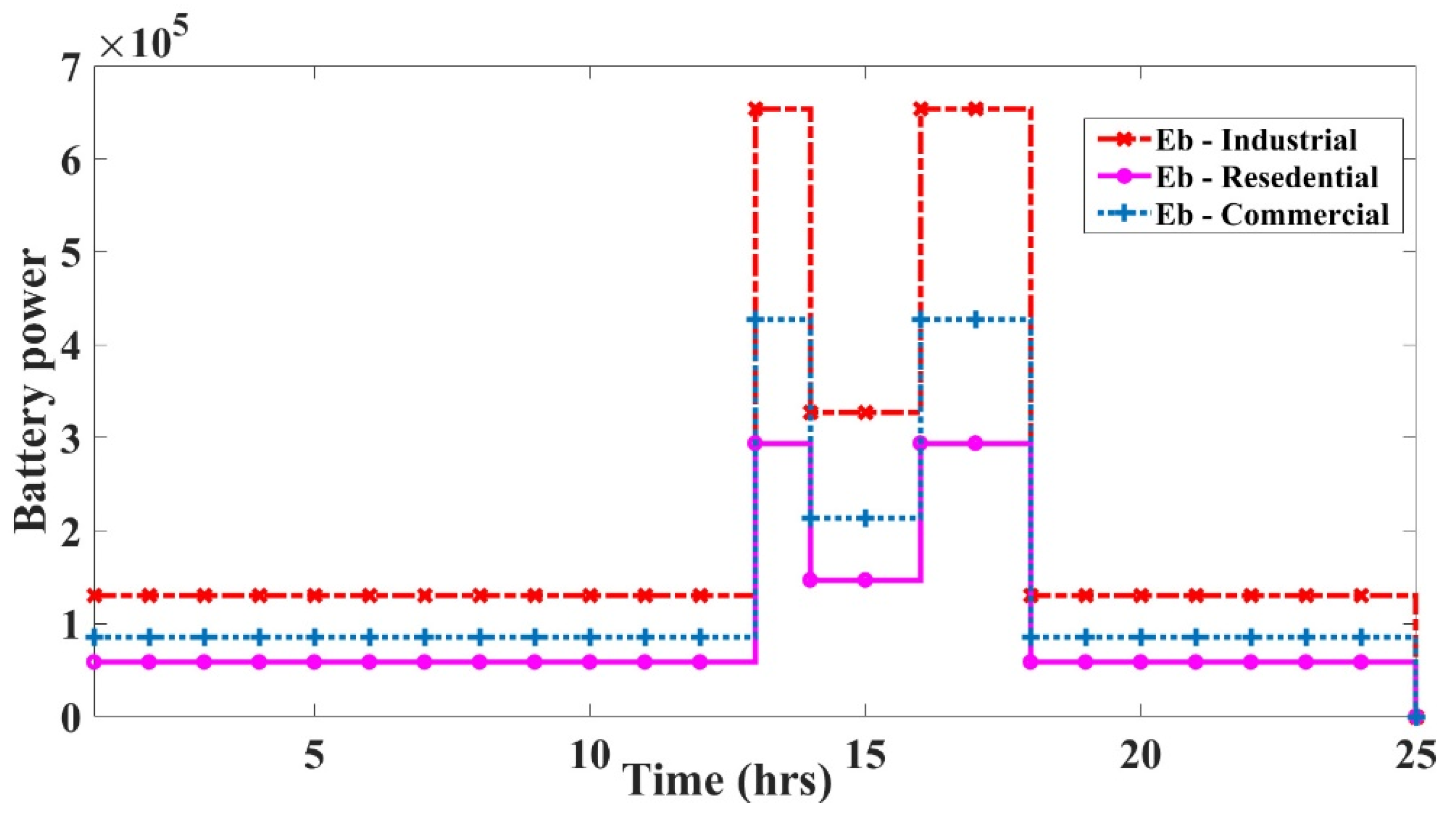
The capacity of a battery storage system is determined by the total demand of the day. As three different types of load profiles were considered in the research, the capacity of the battery was calculated accordingly. The efficiency was estimated to be 95%; the battery’s round trip DC-storage-to-DC energetic efficiency and the state of charge (SOC) under which the battery must never be drawn were 85% and 30%, respectively. The system’s battery capacity (kW) (Figure 5) was measured using the following equation based on demand and autonomy days:

$$CB=\frac{\mathrm{El}\times \mathrm{AD}}{\mathrm{DOD}\times \mathsf{ŋ}inv\times {\mathsf{ŋ}}_{\mathrm{b}}}$$

(33)

where AD is autonomy days, DOD represents depth of discharge (80%), El is the mean of total demand, ŋ_inv is the inverter (95%) efficiency, and ŋ_b battery (85%) efficiency. Battery capacity is chosen to supply power to the consumers for around 6 h in the absence of required renewable energy generation. The battery capacities calculated as per the equation are as given in

Table 2. Battery storage capacities for different loads.

Type of Consumer	Industrial	Commercial	Residential
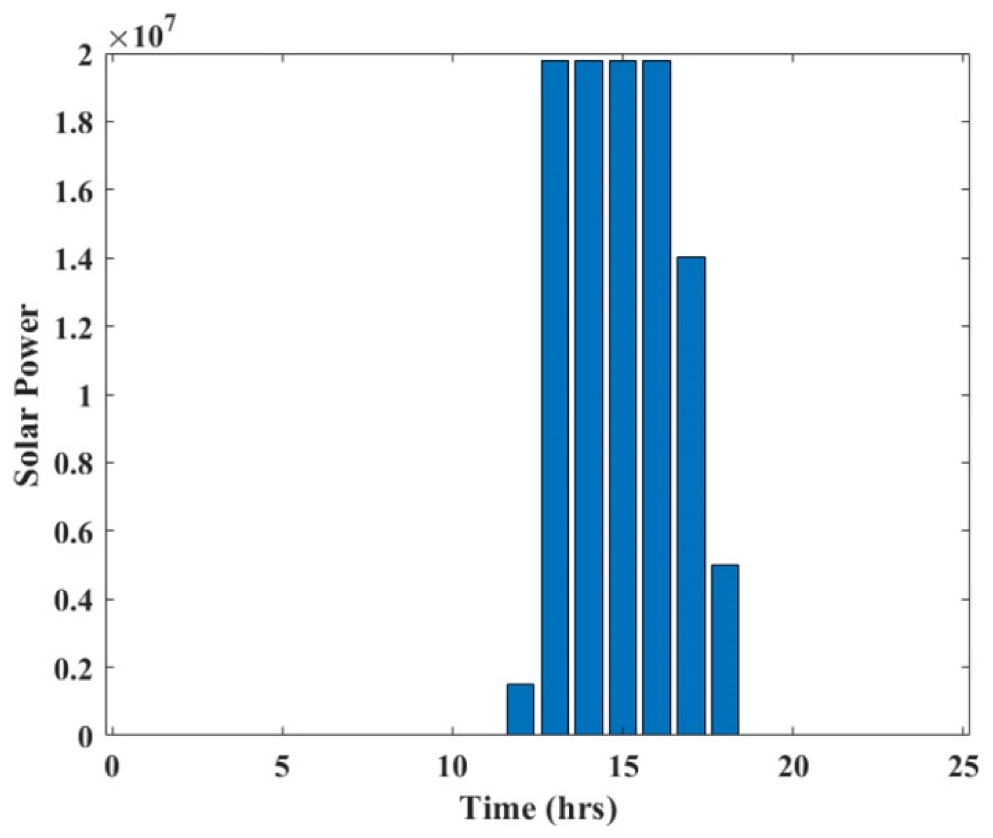
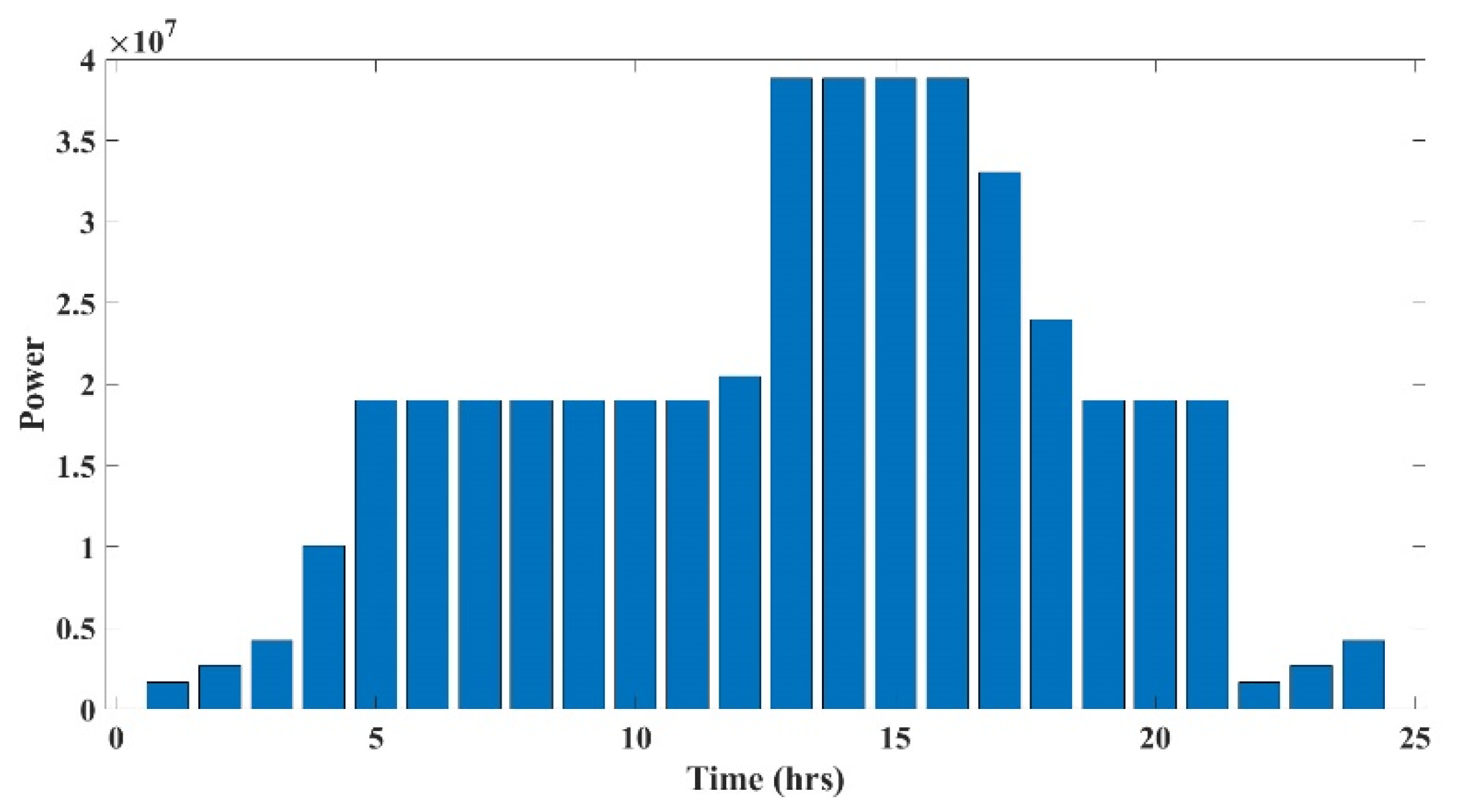
CB	6.54 × 105	4.27 × 105	2.94 × 105

and total renewable power generated was depicted from Figure 6.

3.9. Power Management Algorithm (PMA)

The operating modes and the power to be injected/drawn to/from the IEEE 30-bus six-generator system connected to RESs are decided by the PMA.

The main operational objectives of the PMA are:

▪

To achieve power balance in every operating mode.

▪

To identify the operating mode of the system and make a decision based on demand (PL).

▪

Minimize/maximize power supplied to the grid during peak/off-peak pricing.

▪

To maintain battery SOC within limits.

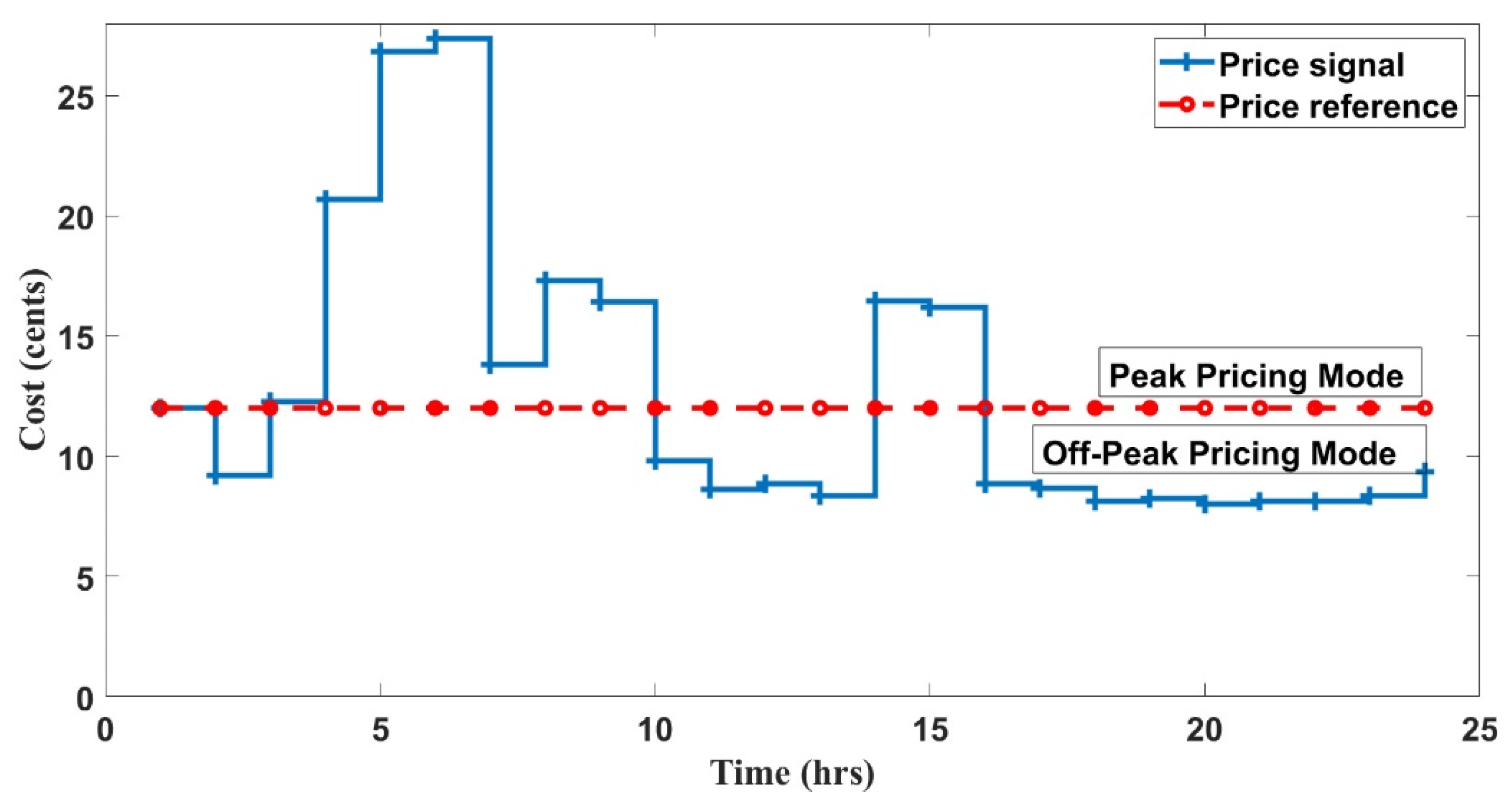
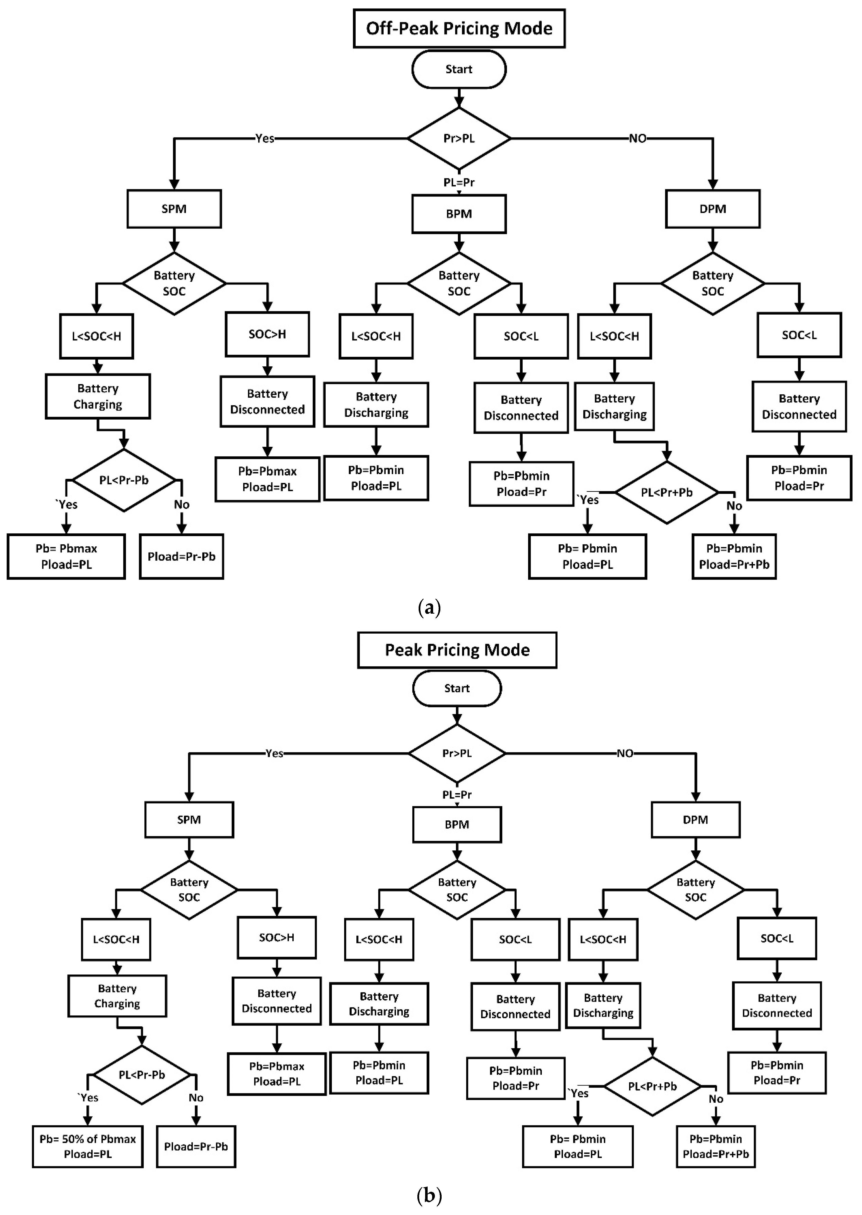
There are two modes of operation based on the cost curve (Figure 7) considered.

3.9.1. Peak Pricing Mode

The battery will be idle or charged up to 50% of its capacity if the SOC value is less than the lower limit (Figure 8a).

3.9.2. Off-Peak Pricing Mode

The battery will be idle or charged up to 90% of its capacity if the SOC value is less than the lower limit (Figure 8b).

Based on the allowable penetration of real power into the grid and its difference with renewable power generated (Pr), these two modes are again subdivided into three modes as follows:

Deficit power mode (DPM; Pr < PL): In this mode, the battery is discharged to satisfy the deficit power, if available; otherwise, only available renewable energy generated is injected into the grid.

Surplus power mode (SPM; Pr > PL): Excess power is supplied to dump load, once the battery is disconnected in this mode; when the higher limit (i.e., SOC > H) of the battery is reached, or the higher limit of the SOC (i.e., L < SOC < H), the battery is charged (L—lower limit, H—upper limit of the SOC of the battery).

Balanced power mode (BPM; Pr = PL): The total renewable power generated is supplied to the grid in this mode.

In DPM and BPM, in spite of the charging mode of battery, because of the following reasons, discharging mode is preferred:

(1)

Minimization of system efficiency due to feeder losses if the battery is selected in charging mode because, compared to the grid, the battery system is nearer to load centers.

(2)

The burden on the feeder is reduced by selecting the discharging mode of the battery. However, battery charging mode is also preferred if the grid has lower transmission losses.

4. Optimization Techniques

This section examines PSO, FA, and HFPSO algorithms and their trademark and how they solve the objectives of the present work in three unique industrial, commercial, and residential areas.

4.1. Particle Swarm Optimization Algorithm

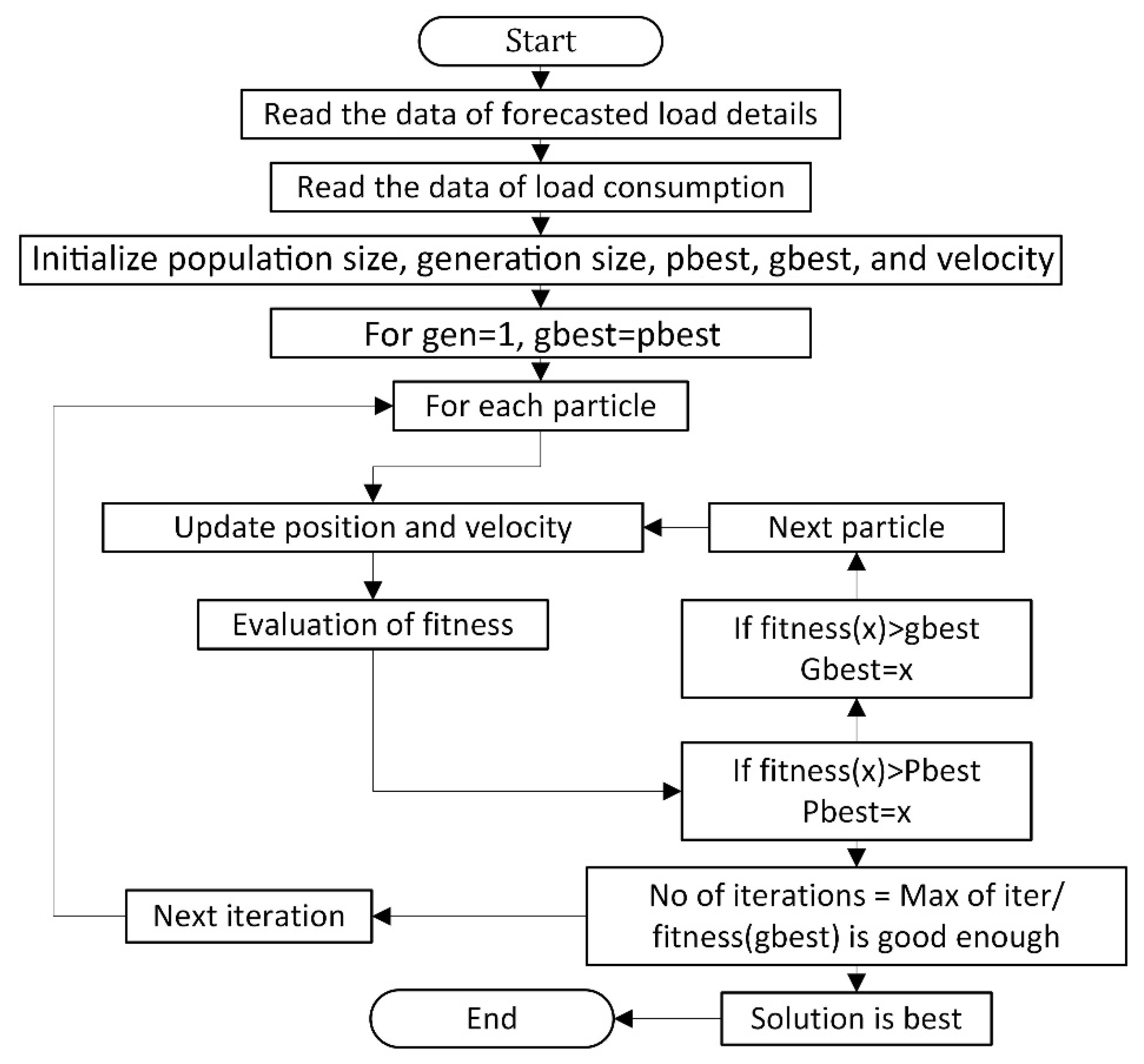
In 1995, Kenney and Eberhart proposed PSO. Two concepts inspired it: the field of evolutionary computation and the theory of swarm intelligence, which focuses on the social interaction that swarms exhibit. The two best values determine the location of each particle in the PSO algorithm. The first is the particle’s best value, also called personal best, stored. The other is called global best, which is obtained by the PSO optimizer among the populations. Each particle location represents the value of variables and the velocity used to find personal and global best values (Figure 9). The proposed PSO algorithm works by keeping many particles solution-searching in the search space at the same time.

Each particle solution is evaluated by using the objective function that is being optimized during each iteration of the PSO algorithm using parameters as shown in

Table 3. Parameters of PSO.

Population Size	50
ωmax	0.99
ωmin	0.85
C1, C2	0.12, 1.2
Iteration	50

, which is used to find its fitness value.

The following three steps are repeated until stopping criteria are fulfilled:

• Determine the fitness value of each particle.
• Update personal and global best fitness values and positions of each particle.
• Update particle position and velocity.

The position and velocity of each particle are updated by using the following equation, respectively:

$$V_i\left(t+1\right)=w{V}_i\left(t\right)+c_1{r}_1\left(pbes{t}_i\right(t)-X_i\left(t\right))+c_2{r}_2\left(gbest\right(t)-X_i\left(t\right))$$

(34)

$$X_i\left(t+1\right)=X_i\left(t\right)+V_i\left(t+1\right)$$

(35)

4.2. Firefly Algorithm

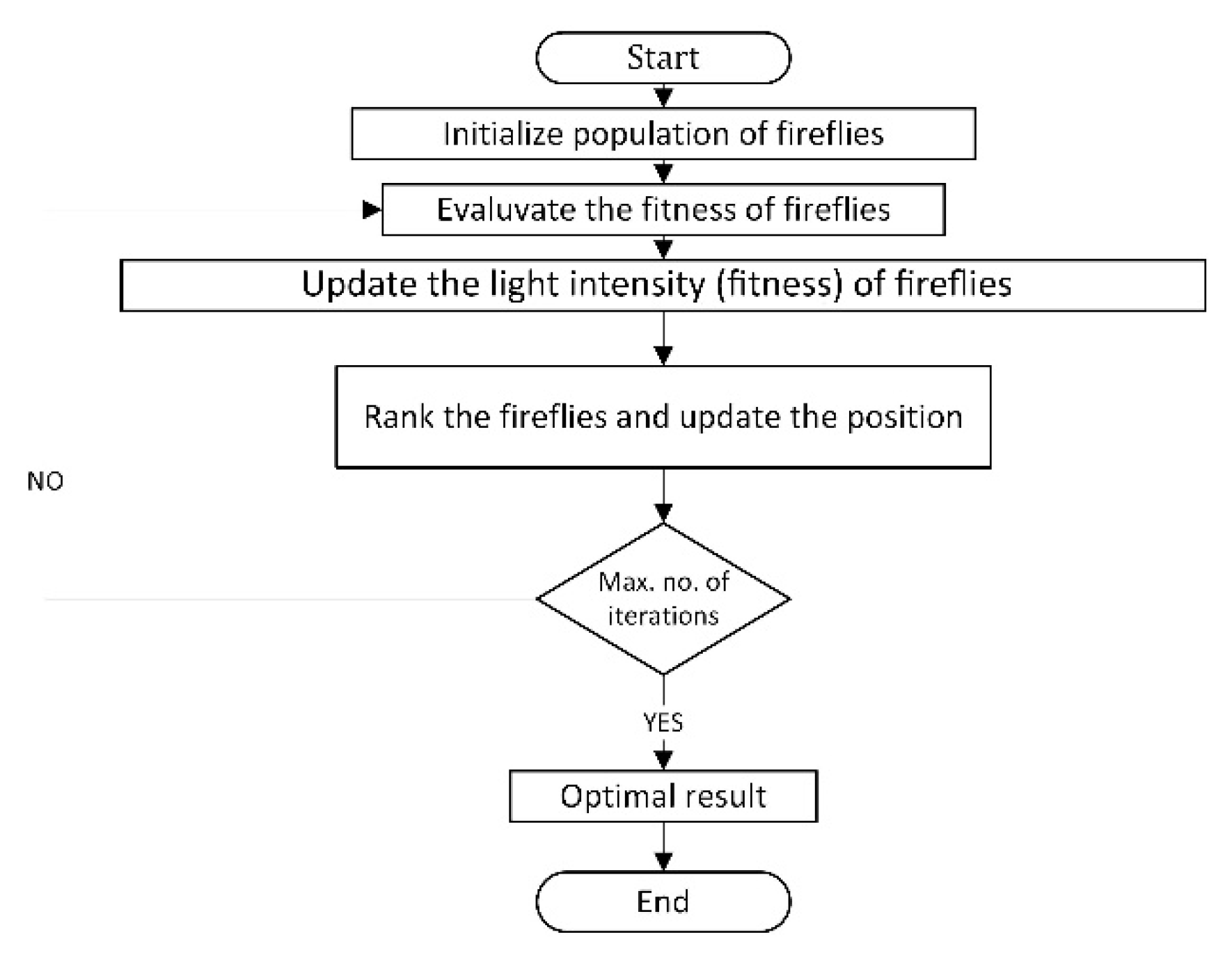
Meta-heuristic algorithms play an important role in today’s global optimization, computer intelligence, and software systems. The multiple agents of interaction usually inspire these algorithms.

In late 2007 and 2008, at the University of Cambridge, Xin-She Yang developed a firefly algorithm (FA)—firefly behavior based on flashing patterns. Essentially, the FA uses three idealized rules:

All fireflies are unisexual; thus one firefly attracts others irrespective of sex.

Attraction is proportional to luminosity, and thus the lighter one moves to the light for each of the two blinkers. With their distance increasing, their appeal is diminishing. It will be altered if there is nothing brighter than a firefly.

The objective function determines the brightness of the fireflies. For a maximization problem, brightness may be proportional to the value of the objective function.

The distance between each firefly i to the j can be the distance of the Cartesian X_i from X_j, $r_{ij}=X_i-X_j$.

The light intensity I(r) varies monotonically and exponentially with the distance in a simple form.

$$I=I_o\times e^{-\gamma r_{ij}}$$

(36)

As a firefly’s attraction is proportionate to the intensity of light seen by neighboring fireflies, the attraction variance β can now be determined with distance r by

$${\mathsf{\beta }=\mathsf{\beta }}_{\mathsf{O}}{\mathrm{e}}^{-{\mathsf{\gamma }\mathrm{r}}^2}$$

(37)

where β_o is the attractiveness at r = 0. The movement of a firefly i attracts another more attractive (brighter) firefly j which is determined by

$$x^{\mathrm{t}+1}=x_i^t{+\mathsf{\beta }}_{\mathsf{O}}{\mathrm{e}}^{-{\mathsf{\gamma }\mathrm{r}}^{2}ij}(x_j^t-x_i^t)+{\alpha }_t{\in }_i^t,$$

(38)

The second term is due to attraction. The third term is randomization, with αt being the randomization parameter. If ${\mathsf{\beta }}_{\mathsf{O}}$ = 0, it becomes a simple random walk. On the other hand, if γ = 0, it reduces to a variant of particle swarm optimization (Figure 10) using parameter values as shown in

Table 4. Parameters of FA.

No. of Iterations	100
Light absorption coefficient	0.5
Attractiveness coefficient	0.2
Scaling factor	0.1

.

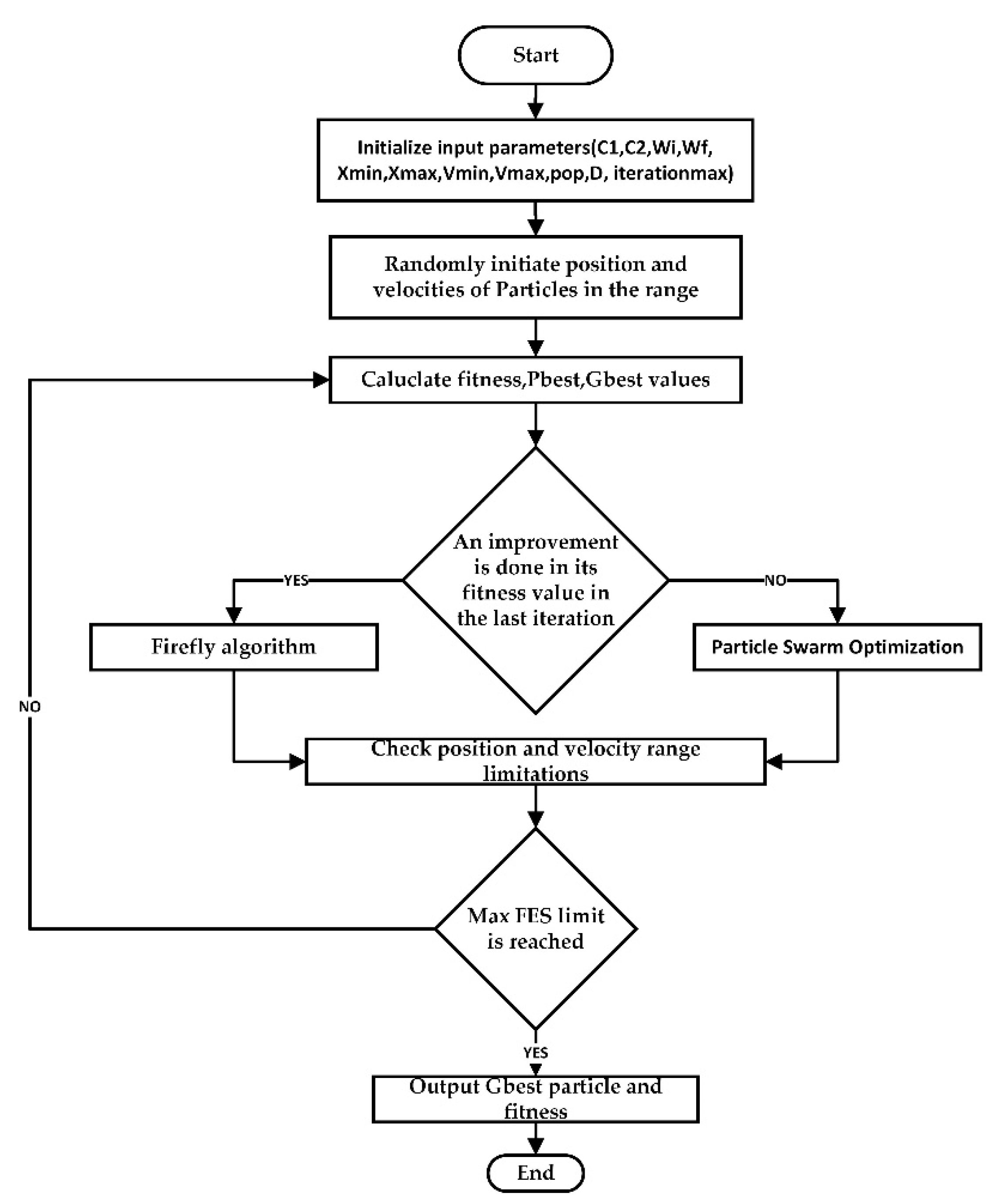
4.3. Hybrid Firefly and Particle Swarm Optimization (HFPSO) Algorithm

This algorithm incorporates the discoverability of firefly and particle swarm optimization algorithms into an optimization algorithm. Therefore, the goal of a balance between exploitation and exploration is to develop and gain the advantages of both algorithms [27,28]. As opposed to particles, fireflies have no personal best location (pbest) memory and velocity (V). In the hybrid version of the two algorithms, PSO offers rapid convergence in exploration as it is commonly used in global search. In fact, for local search, the FA is commonly used as it allows tweaking for exploitation. Dynamic inertia weight tests, which find enhancements to previous personal best, have been successful [29]. The flowchart of the HFPSO algorithm is shown in Figure 11. In the initial step, the input variables used for both algorithms are used. Next, predefined velocity and search limit particle vectors are uniformly prepared. The global best (gbest) and personal best (pbest) of particles are measured and distributed. During the next step of evaluation, in the last iteration, according to Equation (40), it is determined if the sample increased its fitness value. Then, according to Equations (34) and (35), the present state is transferred to a temporary variable (Xi temp), and a new location and velocity are measured.

$$w=wi-\left(\left(wi-wf\right)/iterationmax\right)\times iteration$$

(39)

$$\mathrm{f}\left(i,\mathrm{t}\right)=\{\begin{array}{c}yes,iffitness\left(\mathrm{particle}\left(\mathrm{t},\mathrm{i}\right)\right)\le gbest\left(\mathrm{t}-1\right)\\ No,iffitness\left(\mathrm{particle}\left(\mathrm{t},\mathrm{i}\right)\right)>gbest\left(\mathrm{t}-1\right)\end{array}$$

(40)

Therefore, if the particle has a superior or equivalent fitness value than the prior global maximum, it is presumed that the local search begins. An imitative FA treats the particle; otherwise, the particle will be treated by PSO, and it will begin its regular processes for this particle according to Equations (34) and (35), respectively. During the next step of the analysis, both particles and fireflies were tested for fitness function tests and range limits. A hybrid algorithm provides the gbest and fitness values when the full iteration limit is reached. A total number of fitness function evaluations (MaxFES) is used; in evolutionary computation, MaxFES is a common termination criterion that enables full measurement of objective functions [7]. Exploration and exploitation are balanced by the inertia weight (w) parameter in PSO. Normal declining weight of inertia is used and measured according to Equation (39) [24]. Maximum and minimum particle velocity (Vmin, Vmax) is used in the direction to restrict the next step. The hybrid algorithm is arbitrarily placed within the velocity range at the beginning.

Simple PSO and FA algorithms are comparable to the current HFPSO algorithm. The swarm (pop) size was calculated to be equal in the algorithms. Thus, it is provided that the maximum iteration size is equal in simulations.

5. Results and Discussion

The IEEE 30-bus network with six generators was introduced here. The cumulative load amounted to 285.895 MW. The generation limits of active power and unit costs of all IEEE 30-bus generators are shown in

Table 5. For economic dispatch.

Units	ai USD/h	bI USD/MW·h	Ci USD/MW2·h	Pmin (MW)	Pmax (MW)
01	10	200	100	5	50
02	10	150	120	5	60
03	20	180	40	5	100
04	10	100	60	5	120
05	20	180	40	5	100
06	10	150	100	5	60

and

Table 6. For emission dispatch.

Units	Ai	βi	γi
01	4.091	−5.554	6.490
02	2.543	−6.047	5.638
03	4.258	−5.094	4.586
04	5.326	−3.550	3.380
05	4.258	−6.047	4.586
06	6.131	−5.555	5.151

. All these data are standard data. In three distinct areas, load shifting was performed, and simulation was executed with the DSM methodology. Various kinds of customers have a diverse number of controllable gadgets and measures of energy utilization, as detailed in

Table 7. Types of loads.

Areas	Type of Loads	Controllable Devices	Maximum Load Demand (MW)	Connection Length (km)
Residential	14	2604	1.5	2
Commercial	8	808	2	3
Industrial	6	109	3	5

(limits of power generation and cost coefficients for six-generator unit systems).

Smart grid was connected to mains by a reactance of 0.01 pu and the resistance of 0.003 pu, and 500 KVA was the maximum power transfer limit. Twelve hours were taken as the maximum allowable delay for the simulation.

5.1. Simulation Results

A combined economic emission dispatch problem was solved for a six-generator bus system by integrating renewable energy sources such as solar thermal and wind and wave by incorporating a power management algorithm and demand-side management strategy with different combinations and for three different types of controllable loads for effective reduction in peak-load demand, fuel cost, and emission of thermal plants. The load profiles were adjusted at the peak hour, and thus generous savings were accomplished by turning on a significant expense generator. A detailed analysis of the objectives was carried out by PSO, FA, and HFPSO techniques by implementing the PMA following a day-ahead pricing scheme for RES output according to the available penetration (10%) into the grid.

5.2. CEED

For the considered IEEE 30-bus six-generator system, fuel cost and emission values without considering RESs and DSM are detailed in

Table 8. CEED without RES and DSM (PD = 285.895 MW).

Algorithm	P1 (MW)	P2 (MW)	P3 (MW)	P4 (MW)	P5 (MW)	P6 (MW)	PG (MW)	Fuel Cost (USD/h)	Emission (kg/h)
PSO	17.709	30.446	59.007	97.894	52.111	35.655	292.824	621.743	20.3443
FA	13.584	30.133	58.24	98.344	52.601	35.438	288.349	611.367	20.3125
HFPSO	14.096	29.893	57.495	98.101	51.055	35.252	285.895	605.912	20.1445

, by solving the objectives using PSO, FA, and HFPSO techniques.

5.3. CEED Considering RESs

The renewable sources solar thermal, wind, and wave energy sources and thermal and battery storage systems were evaluated by the authors in this work. Six generators were connected to an IEEE 30-bus hybrid power system, showing real-time data of temperature, solar radiation, wind velocity, wave height, and time period of waves of Gujarat.

The PMA takes the responsibility of observing the power output of the RESs connected to the grid to not exceed the allowed tolerance level and considering the day-ahead pricing schemes to charge the BESS following the modes of operation PPM and off-PPM. By the introduction of RESs, the share of load met by these sources is reduced from the load to be met by thermal generators. Hence, the load on generators following fuel consumption will be reduced, reducing fuel cost and emission output from the system. The details are tabulated in

Table 9. CEED with RESs (PD = 285.895 MW).

Algorithm	Best Fuel Cost (USD/h)	Mean Fuel Cost (USD/h)	Max Fuel Cost (USD/h)	Best Emission (kg/h)	Mean Emission (kg/h)	Max Emission (kg/h)
PSO	548.4902446	573.8555938	608.9511054	19.86406382	20.38286265	20.50344343
FA	568.2427749	590.0721075	621.695385	20.07339404	20.13514927	20.22631838
HFPSO	548.3739915	573.6874823	607.4102221	20.32325434	20.39798968	20.46253179

. By comparing the results of PSO, FA, and HFPSO, for hourly varying RESs for 24 h, the mean values were considered, and the maximum and best values of fuel cost and emission output were considered.

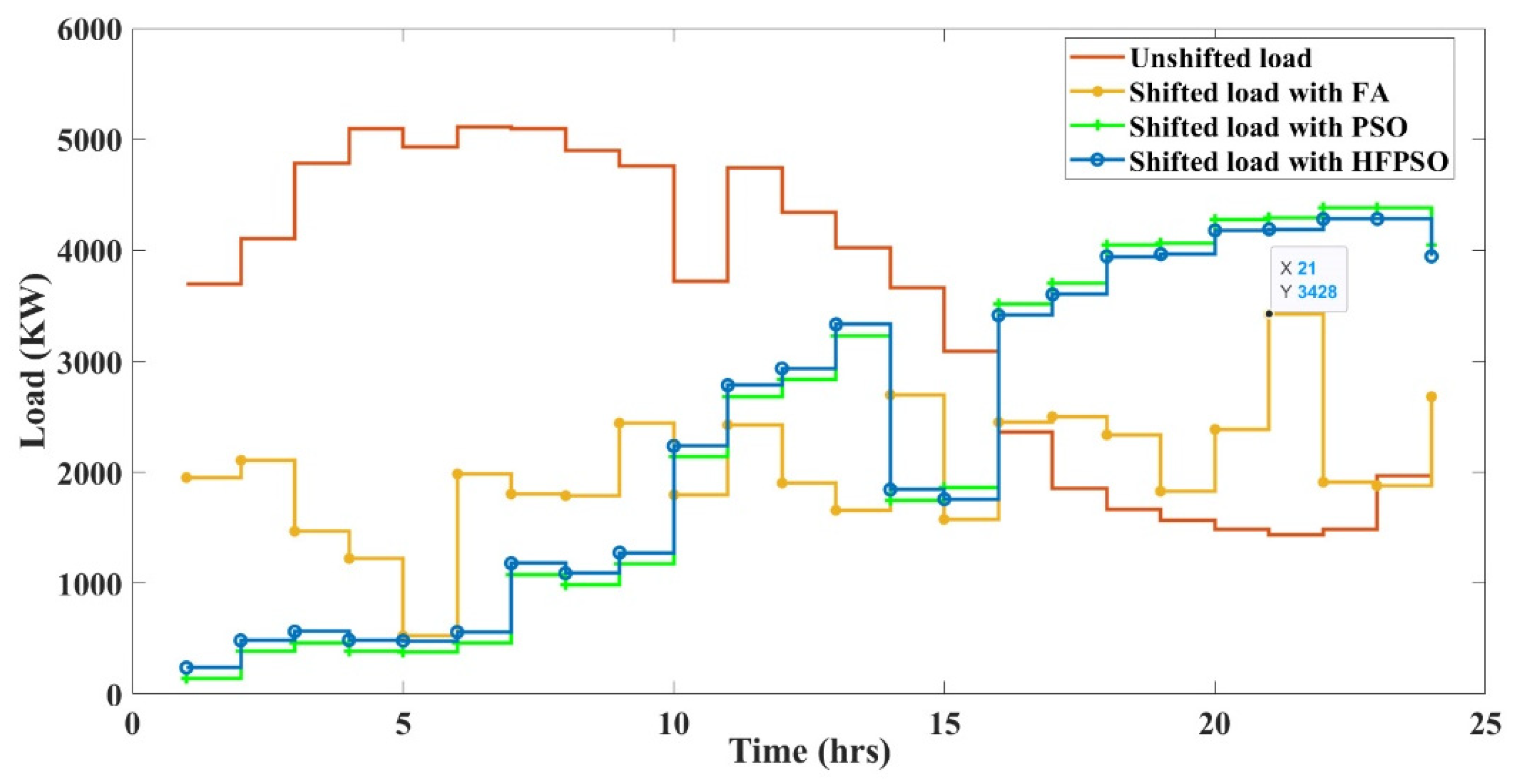
5.4. CEED Considering DSM

The paper’s primary objective and demand-side management strategy for three different zones of loads (residential, commercial, and industrial) were considered under a total load of 285.589 MW. As explained in Section 3, following the cost curve, the load consumption was scheduled to reduce the peak-load hours, reducing the burden on the generators, which results in the reduction of fuel consumption and emission output from the considered system for a period of 24 h. The objective function values are given in

Table 10. CEED with DSM (PD = 285.895 MW).

Algorithm	Best Fuel Cost (USD/h)	Mean Fuel Cost (USD/h)	Max Fuel Cost (USD/h)	Best Emission (kg/h)	Mean Emission (kg/h)	Max Emission (kg/h)
PSO	602.0821181	609.0444743	617.1014456	19.86406382	20.19576052	20.47849924
FA	613.1473332	620.8282859	630.3062173	20.07339404	20.12262237	20.18782291
HFPSO	601.6286714	608.5412088	616.8116302	20.30104453	20.32212451	20.33333378

and

Table 11. CEED with RES and DSM (PD = 285.895 MW).

Algorithm	Best Fuel Cost (USD/h)	Mean Fuel Cost (USD/h)	Max Fuel Cost (USD/h)	Best Emission (kg/h)	Mean Emission (kg/h)	Max Emission (kg/h)
PSO	544.8071922	571.348123	614.152987	20.2501018	20.3811850	20.5337736
FA	559.8734913	587.138890	621.695385	20.0701481	20.1380997	20.2398263
HFPSO	544.1608511	571.140969	614.048243	20.3010445	20.4094863	20.4873394

, which give the details of the peak reduction of three different zones of loads by employing DSM strategy using PSO, FA, and HFPSO.

5.5. CEED Considering RES and DSM

In the above sections, it is clear that the integration of RESs and considering DSM show a considerable impact in the reduction of peak-load demand individually. Now, considering the minimization of objectives, when both impacts were considered at once for a period of 24 h, the variability of parameters of RESs and varying cost considered by DSM come into the scenario at the same instant, which helps in further reduction of burden on the thermal generator system which results in further reduction of fuel cost and emission output; the results are tabulated in

Table 12. Peak-load variation of individual loads.

Peak Load (KW)
Consumer Type	Without DSM	With DSM
		PSO	% Reduction	FA	% Reduction	HFPSO	% Reduction
Residential	1363.6	939.59	31.094	1249	8.4042	936.89	31.292
Commercial	1818.2	1380.8	24.056	1428.9	21.411	1378	24.210
Industrial	2727.3	2074	23.954	1332.5	51.142	1331	51.197

and

Table 13. PAR variation of total load.

Algorithm	PAR	Difference	Reduction (%)
Unscheduled	1.8	-	-
PSO	1.6	0.2	11.11%
FA	1.4	0.2	11.11%
HFPSO	1.2	0.2	11.11%

showing the reduction of the peak-to-average ratio (PAR) of the total load by PSO, FA, and HFPSO, respectively.

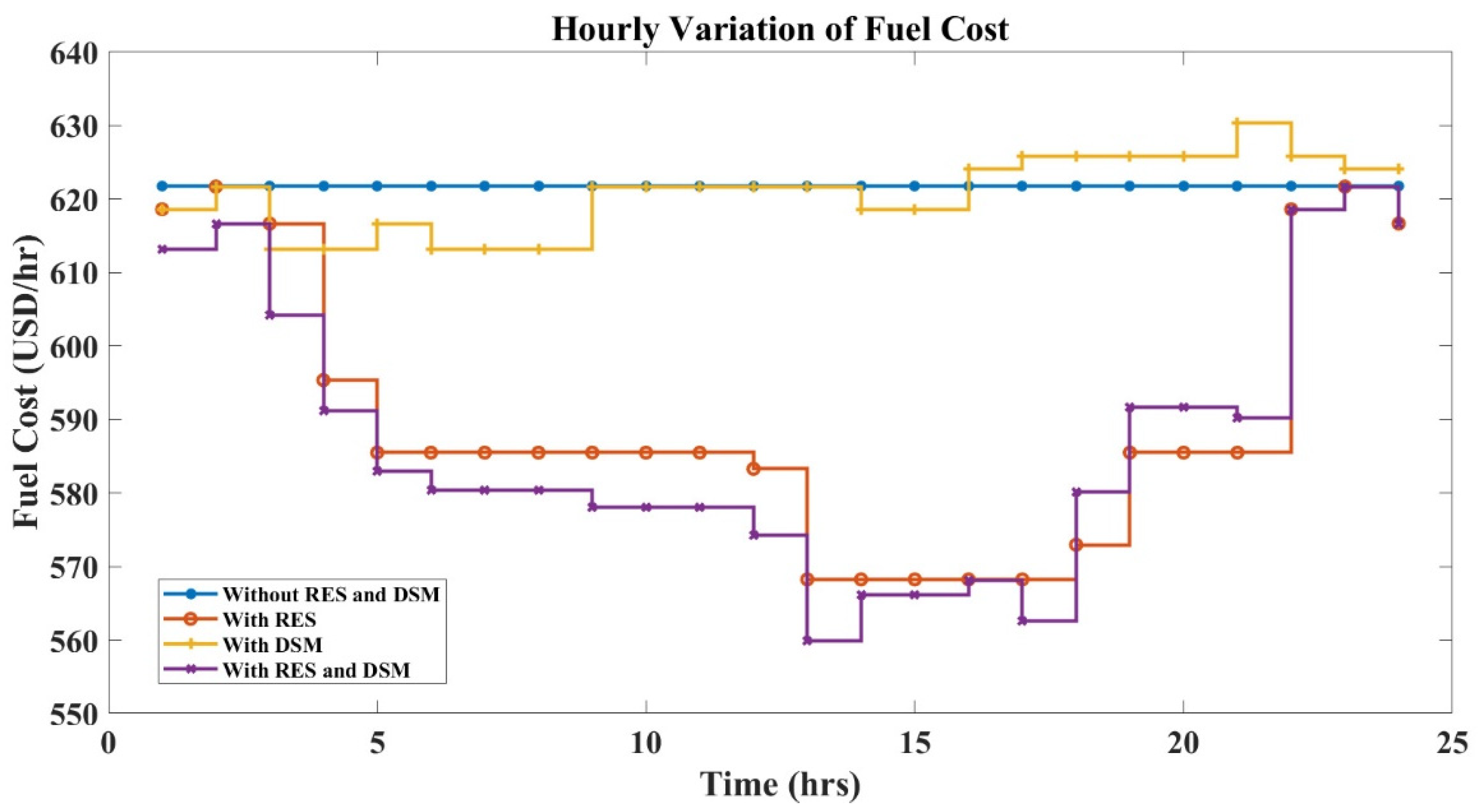
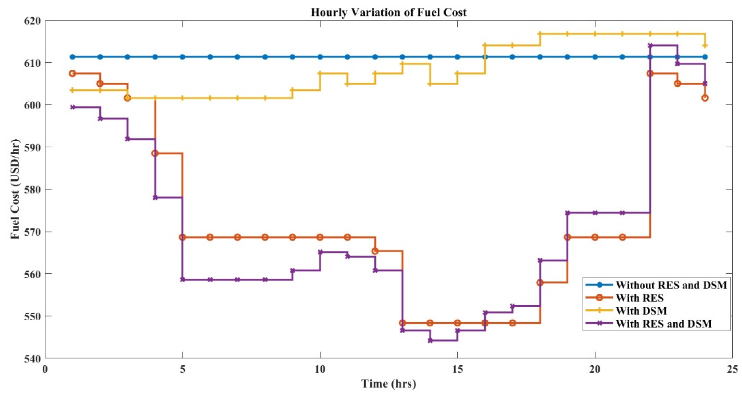
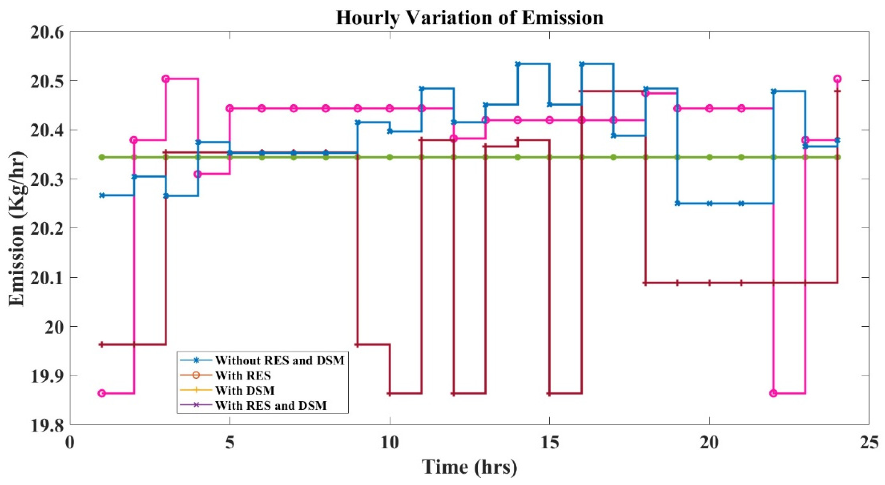
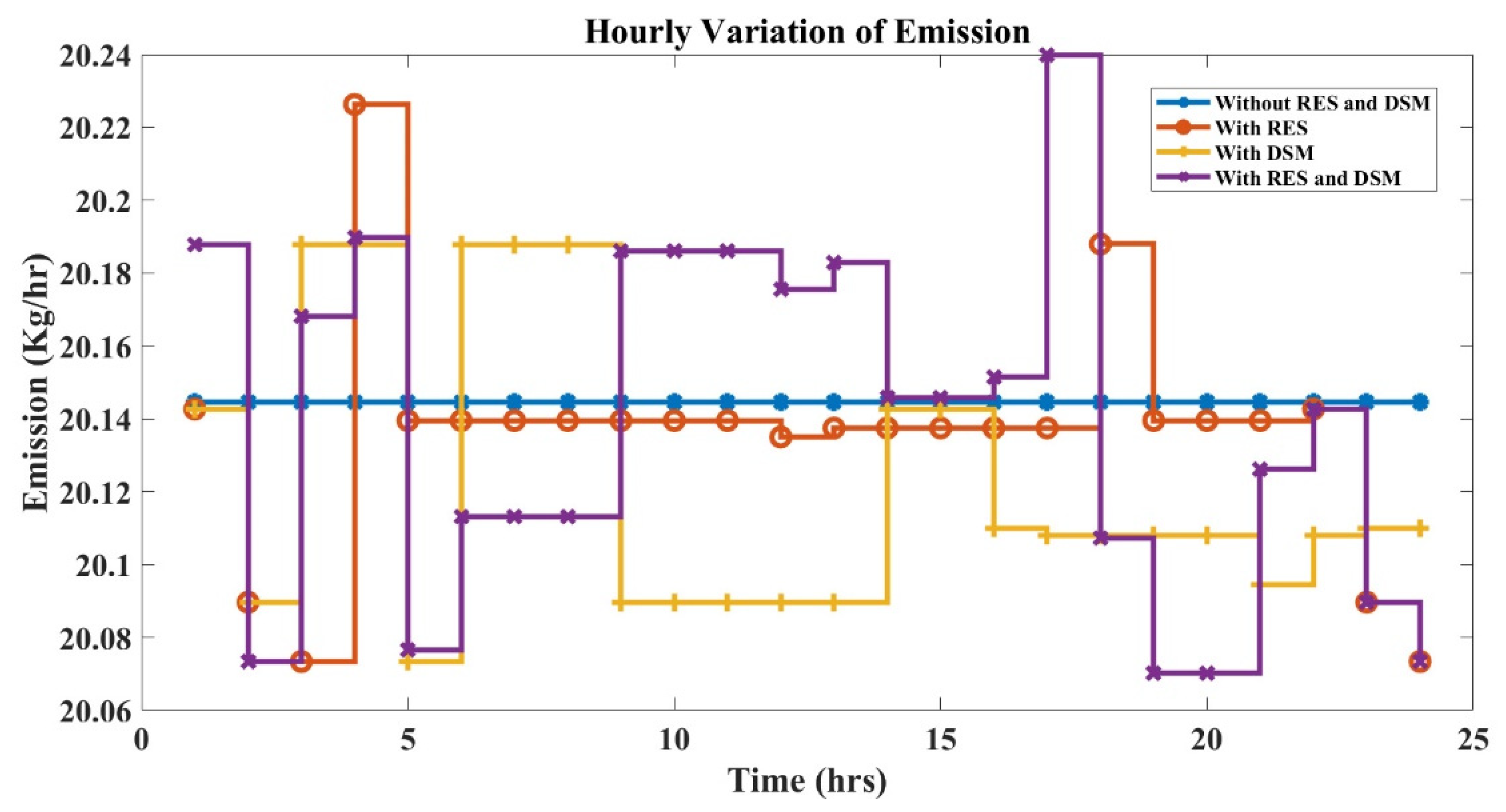
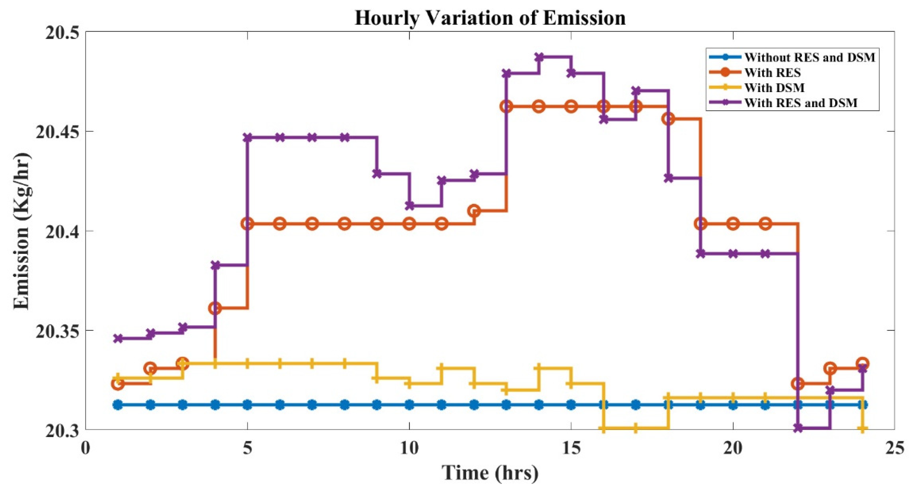
The graphical representation of objective functions further supports the above analysis. Figure 12 represents the variance of total load corresponding to three controllable zones (residential, commercial, and industrial). Figure 13, Figure 14 and Figure 15 represent the hourly variation of fuel cost, and Figure 16, Figure 17 and Figure 18 represent the hourly variation of the emission output of the six-generator IEEE 30-bus system for a period of 24 h using PSO, FA, and HFPSO. 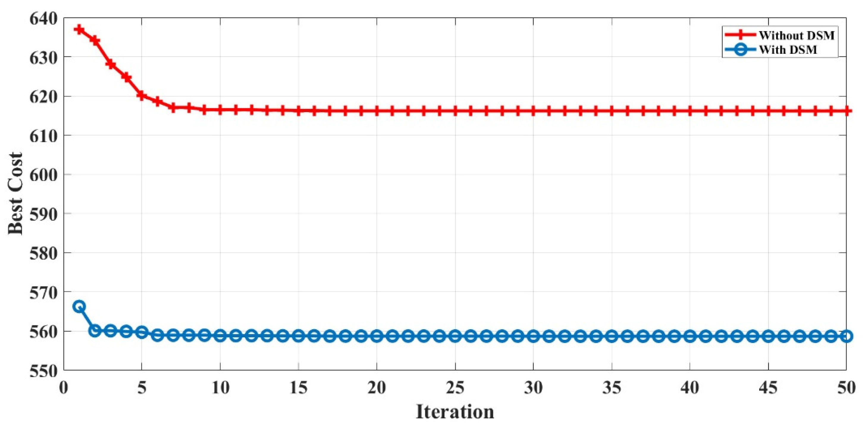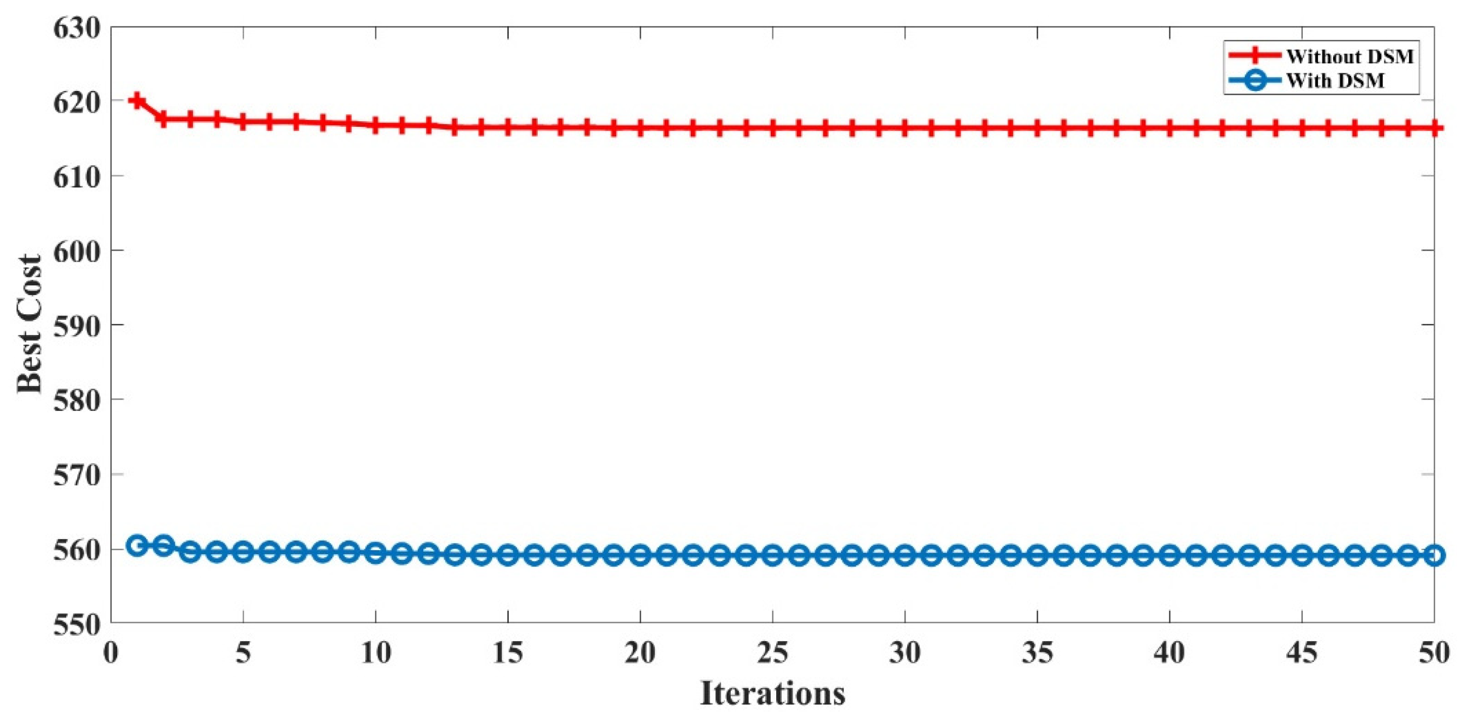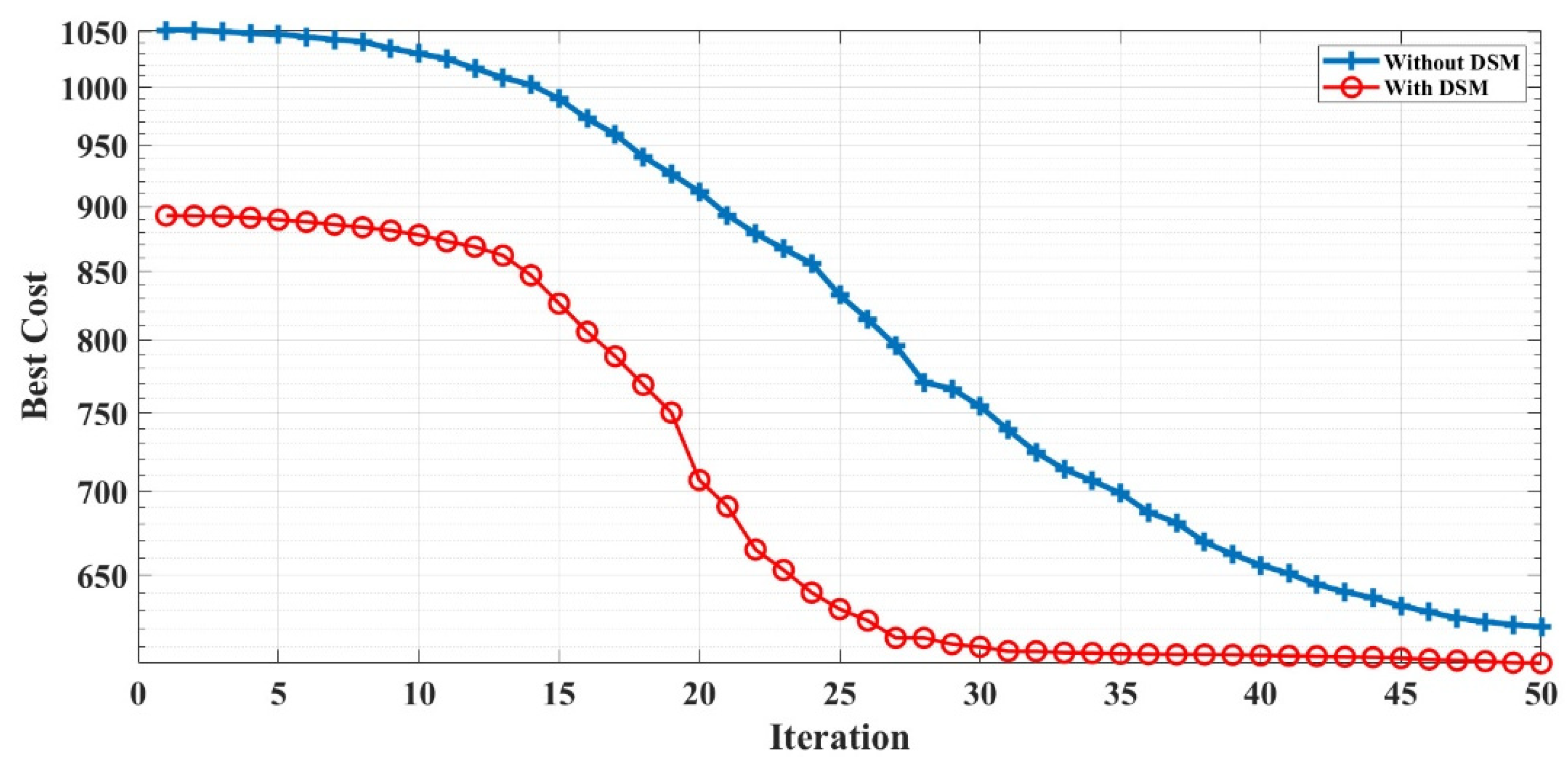Figure 19, Figure 20 and Figure 21 support the performance of HFPSO compared to PSO and FA showing the best results in convergence plots for implementing DSM strategy.

6. Conclusions and Future Work

In this paper, three techniques (PSO, FA, and HFPSO) were applied to solve a day-ahead demand-side-management-integrated hybrid-power-management-incorporated combined economic and emission load dispatch (CEED) problem considering losses. The real-time data of Gujarat were considered when solving the objectives. The comparative performance indicates that the HFPSO manages the process of exploration and exploitation and hence is found to be superior among the three techniques giving the best outcomes of fuel cost 544.160 (USD/h), emission 20.301 (kg/h), and peak-load reduction of 31.292%, 24.210%, and 51.197% for residential, commercial, and industrial loads, respectively. DSM does not just deal with the demand side; it is also beneficial for the generation side, and there are numerous DSM procedures used to oversee and utilize the supply power. Perhaps the best DSM strategy is the load-shifting method. DSM additionally diminishes the service bill and environmental contamination. The proposed power management algorithm effectively manages the allowable renewable generation along with thermal and battery storage systems to balance the load and generation based on the day-ahead pricing scheme. In our future work, we shall compare the performance of the proposed power management algorithm with some other recent algorithms. Furthermore, we shall consider the integration of different RESs and storage options to enhance the reliability of the power system.