Article

Assessment of Climate Change Impact on Snowmelt Runoff in Himalayan Region

1
College of Agricultural Engineering and Technology, Shalimar Campus, Sher-e-Kashmir University of Agricultural Sciences and Technology of Kashmir, Srinagar, Jammu and Kashmir 190025, India
2
Department of Irrigation and Drainage Engineering, College of Technology, G. B. Pant University of Agriculture and Technology, Pantnagar, Uttarakhand 263145, India
3
Civil, Environmental and Natural Resources Engineering, Lulea University of Technology, 97187 Lulea, Sweden
4
Division of Agricultural Engineering, ICAR-Indian Agricultural Research Institute, Pusa Campus, New Delhi 110012, India
5
Agricultural Engineering Department, Faculty of Agriculture, Mansoura University, Mansoura 35516, Egypt
6
Agricultural and Food Engineering Department, IIT–Kharagpur, West Bengal 721302, India
7
Water Technology Center, Indian Agricultural Research Institute, New Delhi 110012, India
8
CERIS, Instituto Superior Técnico, University of Lisbon, 1649-004 Lisbon, Portugal
*
Authors to whom correspondence should be addressed.
Sustainability 2022, 14(3), 1150; https://doi.org/10.3390/su14031150
Submission received: 25 November 2021 / Revised: 13 January 2022 / Accepted: 14 January 2022 / Published: 20 January 2022
(This article belongs to the Section Environmental Sustainability and Applications)

Abstract

:
Under different climate change scenarios, the current study was planned to simulate runoff due to snowmelt in the Lidder River catchment in the Himalayan region. A basic degree-day model, the Snowmelt-Runoff Model (SRM), was utilized to assess the hydrological consequences of change in the climate. The performance of the SRM model during calibration and validation was assessed using volume difference (Dv) and coefficient of determination (R2). The Dv was found to be 11.7, −10.1, −11.8, 1.96, and 8.6 in 2009–2014, respectively, while the respective R2 was 0.96, 0.92, 0.95, 0.90, and 0.94. The Dv and R2 values indicate that the simulated snowmelt runoff closely agrees with the observed values. The simulated findings were assessed under three different climate change scenarios: (a) an increase in precipitation by +20%, (b) a temperature rise of +2 °C, and (c) a temperature rise of +2 °C with a 20% increase in snow cover. In scenario (b), the simulated results showed that runoff increased by 53% in summer (April–September). In contrast, the projected increased discharge for scenarios (a) and (c) was 37% and 67%, respectively. The SRM efficiently forecasts future water supplies due to snowmelt runoff in high elevation, data-scarce mountain environments.

1. Introduction

The study of the hydrological regime of the catchment is an important and decisive approach in conserving and managing water resources [1,2,3,4]. The hydrological cycle’s key factor and component is the mountain snowpack, which stores winter precipitation and releases it in runoff and streamflow during spring and summer [5,6]. Snow is the primary and most significant water storage component in basins, rendering such places sensitive to global warming and climate change [7]. Climate and streamflow data from mountainous places have shown a pattern of increasing winter minimum temperatures over the last several decades [8] and reduced snowfall compared to the total precipitation [9,10]. It has been indicated that decreased spring snow cover and snow depth [8] affect summer streamflow [11]. Studies in various countries have shown that snow significantly impacts the surface moisture accessible for runoff in the future [12].
In addition to serving as crucial indicators of climatic variability and change, mountain snowpack and spring runoff are major components of surface water resources integrated throughout a large geographic area. As in other parts of the globe, the highest and lowest temperatures recorded in the Kashmir valley during the previous 30 years rose by 1 °C and 0.5 °C, respectively. Climate change impacts such as rising air temperatures decreased snowfall precipitation. Accelerated glacier melt can already be seen in the Himalayan River basins [13], resulting in a significant decrease in the discharge of Himalayan rivers [14]. According to current research programs, the surface temperature increased by 0.74 °C from 1906 to 2005, with warming trends being more prominent in the last 50 years [15]. Kashmir Himalayan glaciers have been melting quickly due to global climate change [2]. Mountains in the Himalayan region are melting at a more rapid rate (0.3–1.0 m/year) than the mean of the world [16].
In predominantly snowmelt basins, the snow-covered area is essential for assessing, modeling, and forecasting meteorological, hydrological, and biological processes [17,18]. Data constraints have hampered thorough knowledge of variability in snow cover and melt in mountainous locations [19]. Snowmelt runoff models are based on various concepts and assumptions. A fitting model is necessary to simulate the snowmelt runoff processes for regions where snowmelt runoff supplies water resources. Over the last four decades, several models have been developed worldwide to represent snowmelt runoff [20,21]. Hydrological models can be as simple as sand-filled boxes or as complex as computer programs. Several criteria can be applied to classify watershed models [22,23]. Snowmelt Runoff Model (SRM) is a theoretical hydrologic model that is most widely used to predict the snowmelt runoff in snow-dominant areas [24].
Jain et al. [5] used the SRM to estimate the runoff due to the rainfall and snowmelt for the Satluj basin, western Himalaya. The model was calibrated for 1996–1999, and the runoff simulation was made for 2002–2005. The study revealed that model efficiency increased with temperature lapse rates. Javadinejad et al. [25] made a similar attempt to analyze the climate change effect on streamflow using the SRM model. The result indicated an increase in temperature and a reduction in snow cover and precipitation. It concluded that most runoffs were generated from snow or ice melting. Modeling snowmelt runoff in data-scarce watersheds using remote sensing data from snow and glacier cover, field measurements, Arc Geographic Information System (GIS) environment, and novel approaches to model parameterization may be viable [26,27]. The socioeconomic indicators are the most important drivers of LULC change and environmental degradation in the catchment [28]. Moreover, the magnitude and intensity of anthropogenic impact are not uniform in different watersheds of the Lidder catchment [28].
Both Ma and Cheng [29] and Yu et al. [30] used the SRM to simulate streamflow in basins in the Tianshan Mountains in China. They found that the model worked well for streamflow modeling and simulation. Immerzeel et al. [31] and Tahir et al. [32] used the SRM model to estimate streamflow in the UIB. They demonstrated that the SRM could simulate daily discharges with high precision. A test carried out in the watershed of the Kuban River basin in Russia showed that the SRM can simulate both diurnal water flow and snow water equivalents in hilly places with high accuracy [33]. Streamflow estimates for short to medium term periods (e.g., 1–15 days) have been generated effectively using the SRM in three snowmelt-dominated basins in Idaho, United States [34], and estimation of discharge using Snowmelt Runoff Modeling in the Upper Kabul River, Afghanistan region [35], Salang River basin, Afghanistan [33], Taleghan watershed, Iran [36], Nuranang river catchment Arunachal Pradesh, India [37], Langtang River basin, Nepal [38], Manasi River basin, China [39], the Karakoram and Himalayan Regions of Pakistan [40], Yurungkash watershed, China [41], and Horo-Dehno watershed, Iran [42]. Nourani et al. [43] studied the snowmelt runoff model (SRM)to estimate the effect of snow on the surface flow of the Aji-Chay basin, northwest Iran, using two calibration techniques to enhance the calibration, applying multi-station calibration (MSC) and single-station calibration (SSC) strategies in order to investigate their effects on modeling accuracy; they found a 15% improvement in model performance with the MSC strategy. Karimi et al. [42] successfully compared the efficiency of the SRM and WetSpa models for snowmelt runoff simulation. They found a Nash–Sutcliffe efficiency of 0.54 and 0.53 for the SRM, compared to 0.77 and 0.8 for the WetSpa in the calibration and validation periods. Siemens et al. [44] studied Runoff Projection using the Snowmelt Runoff Model for an alpine watershed in Western Canada, projecting future runoff in the basin. Yi et al. [45] examined spatiotemporal changes in the snowpack in the Yarkant River Basin (YRB) and the west of Upper Indus Basin (WUIB), associated with the Karakoram Mountains, using the Moderate-resolution Imaging Spectroradiometer (MODIS) daily cloud-free snow cover product from 2002–2018. In both basins, the low-altitude areas experienced a slight decrease in snow cover extent, while the high-altitude areas experienced an increase. Significant elevation dependences were found for the snow cover percentage (SCP), snow covered days (SCD) and snow cover melting dates (SCMD), with an inverse elevation dependence for snow cover onset dates (SCOD) [45]. Keeping in view the modeling importance, this study was conducted with the objectives of detecting a trend of minimum and maximum temperature and precipitation, simulating the streamflow of a basin using the SRM model, and evaluating the performance of the model with climate change scenarios involving the effect of temperature, precipitation, and snow cover on variations in streamflow.

2. Materials and Methods

2.1. Study Area

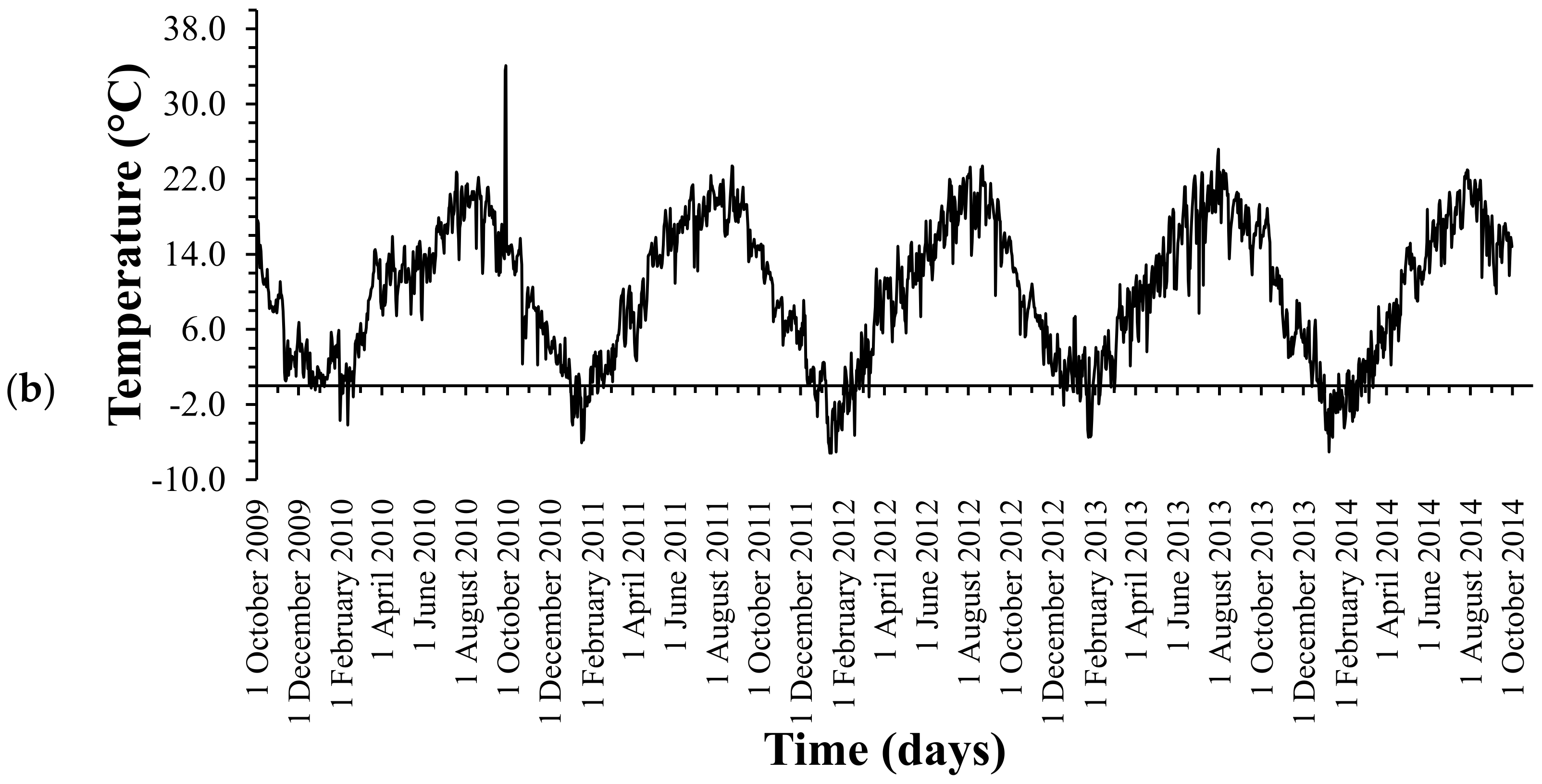
The Lidder watershed, situated in the upper Jhelum catchment, western Himalaya region, was selected in this study. It covers an area of 768 km2 and is located in the longitude of 75°30′ to 75°45′ and latitude of 34°15′ to 34°30′. The catchment area elevation varies from 1800 to 5300 m above mean sea level. This watershed consists of around 3% of the everlasting snow-cover in the whole watershed area, with 6% in the upper watershed. The Lidder watershed features 17 glaciers that encompass an area of around 40 km2 [27]. The largest glaciers of the Lidder watershed are Kolahoi (10.2 km2) and Shishram (8.5 km2) [46,47]. Figure 1 depicts a map of the Lidder catchment location. In the winter (December to March), the catchment receives significant snowfall, melting in the summer. However, the catchment contains permanent snow cover and glaciers, and not all snow in the region melts. Figure 2 depicts the yearly precipitation and temperature observed at the Pahalgam station (a-b). Snow is the most common kind of precipitation throughout the winter season. Although highly variable, the area of snow cover in the Lidder watershed declines from roughly 90% (winter) to about 6% (autumn) [1].

2.2. Snowmelt Runoff Model (SRM)

The SRM is intended to model and estimate streamflow in the snow regions daily, where melting snow plays a significant role in the runoff. Martinec [48] created SRM for small basins. The model can be ascribed to remote sensing of snow cover to cover bigger basins. The important input parameters of SRM are precipitation, air temperature, and percent area snow cover. SRM accounts for degree-days by splitting the watershed into elevation zones to calculate snowmelt. The SRM contained two parts in the present study. The first was to simulate the snow movement to estimate the daily snow cover area and snow storage. The hydrological process included precipitation, snow melting, transpiration, recharge, and discharge accumulation.
The basin was classified into several elevation zones in the SRM. Every day, snowmelt was forecasted in each zone based on rainfall and air temperature. The entire new water was directed through single storage. A single equation can express the model’s original form:
Q n + 1 = kQ n + 1 k ( α i T i A i + P i )  
where Q = discharge from the basin (m3/s), k = recession coefficient, α = degree-day factor [cm °C−1 d−1] indicating the snowmelt depth from one degree-day, T = air temperature (°C) extrapolated to the hypsometric mean height of each zone, A = current snow-covered area in the zone (% of zone area), P = precipitation (mm) falling as rain in the zone (When T > Tcrit), n = sequence of the day during the simulation period.
Ti can be extrapolated from the temperature at the base station using a temperature lapse rate, which is implied in Equation (1). SRM version-4 is slightly more sophisticated and includes extra parameters, while the core framework remains constant. Version-4 of SRM is represented by Equation (2), provided below:
Q n + 1 = k n + 1 Q n + 1 k n + 1 C Sn a i T i A i + C Rn P i  
where CSn = correction factor for losses from snowmelt, CRn = correction factor for losses from rainfall.
The following equation represents the current version of SRM:
Q n + 1 = C Sn α n T n + Δ T n S n + C Rn P n A .10,000 86,400 1 k n + 1 + Q n k n + 1  
where ΔT = the adjustment by temperature lapse rate when extrapolating the temperature from the station to the average hypsometric elevation of the basin or zone [°C/d].
Equation (3) starts with a lag of 18 h between the daily discharge and temperature cycles. In this scenario, the n+1th day discharge depends on the measured degree-days on an nth day. Based on basin features, these factors were measured or calculated using empirical regression relationships and hydrological judgment. The snowmelt depth was calculated using the degree-day factor. The degree-day factor for snow was determined by the Snow density data, which is a strong indication of albedo. There was no information known on the snow density in the area. The crucial temperature was calculated based on the type of precipitation. The critical temperature during the snowmelt season is essential for the SRM to determine whether the rainfall or snowfall (T < Tcrit) instantly contributes to runoff.

2.3. Input Data and Parameter

The required inputs for this study were daily precipitation, temperature, and snow-cover, with discharge calculated on this basis. Weather data was collected from the India Meteorological Department, Rambagh. Precipitation is the most spatially variable among all meteorology variables; thus, the precipitation, maximum and minimum temperature were collected from the IMD daily. The maximum and the minimum temperature values were averaged to obtain the daily average temperatures fed into the model. Weather data and observed runoff data for five years (2009–2014) were also fed into the model. Moderate Resolution Imaging Spectroradiometer (MODIS) remote sensing data of snow cover were used to estimate the snow cover percentage from 2009–2014, as explained in detail in Section 2.4. Snow cover measurements in various elevation zones required a Digital Elevation Model (DEM) for computations. The Advanced Spaceborne Thermal Emission and Reflection Radiometer (ASTER) DEM is suitable for high-latitude and steep mountainous locations, which Shuttle Radar Topography Mission (SRTM) does not cover; the ASTER DEM tiles can be downloaded electronically for the Lidder catchment from https://wist.echo.nasa.gov/wist/api/imswelcome/webpage (15 December 2021). The catchment region was extracted using ASTER DEM data and the Integrated Land and Water Information System (ILWIS).
Input parameters of the SRM were degree-day factor, temperature lapse rate, lag time, contributing rainfall area, snow and rain runoff coefficients, and recession coefficients. These factors were produced from measurements and approximated using judgment based on the Himalayas’ hydrological properties, physical laws, and theoretical and empirical regression relationships [49]. Most of the input parameters were dynamic, changing spatially and temporally [24], implying that a particular set of parameters might not be appropriate every year. The range of the SRM input parameters is summarized in Table 1. The parameter values were set in the range presented in the table upon calibration of the model. The simulated runoff values were adjusted close to the observed runoff.

2.4. Snow-Cover Estimation

Because of the substantial spatiotemporal variation in snow cover and the limited data available for the research region, images derived from satellite sensors appeared to be the best source for estimating snow cover [33]. In this investigation, MODIS images were utilized to estimate snow cover. With the launch of MODIS in December 1999, a progressive development was begun in hyperspectral satellite remote sensing. MODIS allows for environmental monitoring by assessing aerosol concentrations and gas traces in the air and mapping the land, sea, and clouds in many spectral bands. MODIS collects data worldwide for every 1–2 days and has a repetition cycle of 16 days.
In this study, we utilized MOD10A2, a MODIS snow product that provides information on the extent of snow coverage in a repeating period of 8 days [50]. Mapping snow cover was a time-consuming task in this study, as satellite images were obtained daily and processed for snow-cover extraction if the study region was cloud-free. The file size was excessive, and a significant number of images were necessary. From January 2009 to December 2014, a total of 264 processed MOD10A2 images were gathered from http://nsidc.org/cgi-bin/snowi/search.pl, 12 September 2021. For all the Hierarchical Data Format (HDF) images, Geo-referencing was carried out. The images for the Lidder River Catchment were re-projected in ArcGIS 10.2 using the WGS 1984 Universal Transverse Mercator (UTM) Zone 43N projection method. If the percentage of cloud cover on a certain day surpassed 20%, the record was removed. For that day, the snow coverage was approximated by linearly interpolating the preceding and accessible cloud-free images. The snow pixels were multiplied by cell area and then converted to square kilometers, with each 8-day interval value divided by the area of the basin and interpolated to obtain the value of daily snow cover.

2.5. Calibration and Validation of Model

Calibration and validation must be carried out before applying the model to a real-world situation. This procedure provides a credible fat co-relates the observed value to a greater extent. Because it takes regional heterogeneity into account, the SRM model has many parameters. These parameters were calculated using a calibration procedure, as they could not be acquired directly from existing data. Calibration was performed manually in the current study by altering input parameters. Following calibration, adequate validation is required for model testing before being utilized under different situations. In the validation procedure, the model parameters defined in the calibration were used. Model prediction performance was evaluated by comparing the findings to the observed data. The data for the hydrological years (October to September) 2009–2010 was used for calibration, while data for hydrological years 2010–2014 was used to validate the model.

2.6. Model Accuracy

The SRM computer program involves the assessment of model accuracy through the graphical representation of the estimated hydrograph and observed runoff. In addition to the plots, the SRM uses two performance indices, the percent volume difference (Dv) and the coefficient of determination (R2) [24,32,51,52,53]. The coefficient of determination is estimated as follows:
R 2 = 1 ( Q obs Q cal   ) 2 Q obs   Q obs 2  
where Q obs = measured daily discharge, Q cal = simulated daily discharge, Q ¯ obs = average measured discharge.
R2 value shows that the measured and simulated (calculated) values coincide perfectly and plot as 1:1 [53]. The Dv is computed as follows:
D v % = V obs V cal V obs × 100  
where V obs = the measured melting season runoff volume, V cal = the computed melting season runoff volume. A negative Dv value indicates under-estimation of the streamflow, whereas a positive value indicates overestimating.

2.7. Climate Change Impact Detection

The variance of streamflow in mountainous areas is primarily driven by changes in the space and time distribution of precipitation and melting of snow induced by rising temperatures. The runoff in the Lidder river watershed is mainly caused by snowmelt, making it highly exposed to climate change. Analytical studies revealed that a temperature rise of 1–3 °C in the western Himalayan region could increase glacier melt runoff by 16–50% [54]. Therefore, it is critical to employ accurate hydrological methods to predict runoff caused by the snowmelt, especially in high elevation areas under future scenarios of climate change. Therefore, the SRM was applied to simulate the influence of climate change on Lidder River discharge. Three potential climate change scenarios were constructed in the WinSRM model and are mentioned below.
  • Scenario A: 20% increase in precipitation
  • Scenario B: 2 °C rise in temperature
  • Scenario C: 2 °C rises in temperature and 20% increase in snow cover
In mountainous regions, variation in river discharge is mainly influenced by changes in the spatial and temporal distribution of precipitation and the melting of snow cover and glaciers caused by increased temperature. Therefore, we outlined future climate change scenarios using downscaled GCM simulation data, taking into account the effects of rainfall, snowmelt, and glacier melting on streamflow. There were four situations described.: In scenario 1, the change in cryosphere area was ignored, while the average values of temperature and precipitation were adjusted based on HadCM3 statistical downscaling data (Hadley Centre Coupled Model, version 3) in the SRES A2 scenario.
The shift in the cryosphere area was not taken into account in scenario 2. The mean temperature and precipitation area, on the other hand, were altered as a result of the statistical downscaling findings of HadCM3 in the SRES B2 scenario.
The mean temperature and precipitation in scenario 3 were altered according to the statistical downscaling results of HadCM3 in the SRES A2 scenario. The cryosphere area was expected to expand or decrease by 20%. In scenario 4, the mean temperature and precipitation were adjusted based on HadCM3 statistical downscaling findings in the SRES B2 scenario. The cryosphere area was estimated to grow or shrink by 50%.

3. Results and Discussion

The simulation of runoff produced by the snowmelt and rainfall is crucial for planning water management programs. In this study, streamflow in the Lidder river catchment was simulated by the SRM. The SRM was later run for the hypothetical scenarios of change in climate to investigate its implications on the flow pattern. The investigation results are presented and discussed herein under suitable headlines by providing reasoning based on the available literature and field studies. This study calculates the maximum and minimum monthly, seasonal, and annual trends for rainfall and monthly, seasonal, and annual trends for precipitation using Mann–Kendall techniques. The trend magnitudes are calculated using Sen’s slope estimator in the study area. The Mann–Kendall technique results are presented for the annual, monthly, spring, summer, autumn, and winter seasons in the study area.

3.1. Meteorological Data Trends

3.1.1. Monthly, Seasonal and Annual Minimum Trends

The Z statistics of monthly, seasonal, and annual minimum temperature data obtained by Mann–Kendall are presented in Table 2 and graphically at five different significance levels. A positive (negative) value of Z indicates an upward (downward) trend. The smallest significance level α with which the test shows that the null hypothesis of no trend should be rejected. For the four tested significance levels, the following symbols are used in the template: *** if the trend at α = 0.001 level of significance ** if the trend at α = 0.01 level of significance * if the trend at α = 0.05 level of significance + if the trend at α = 0.1 level of significance If the cell is blank, the significance level is greater than 0.1. The annual and seasonal temperature trends for the study area are shown in Figure 3.
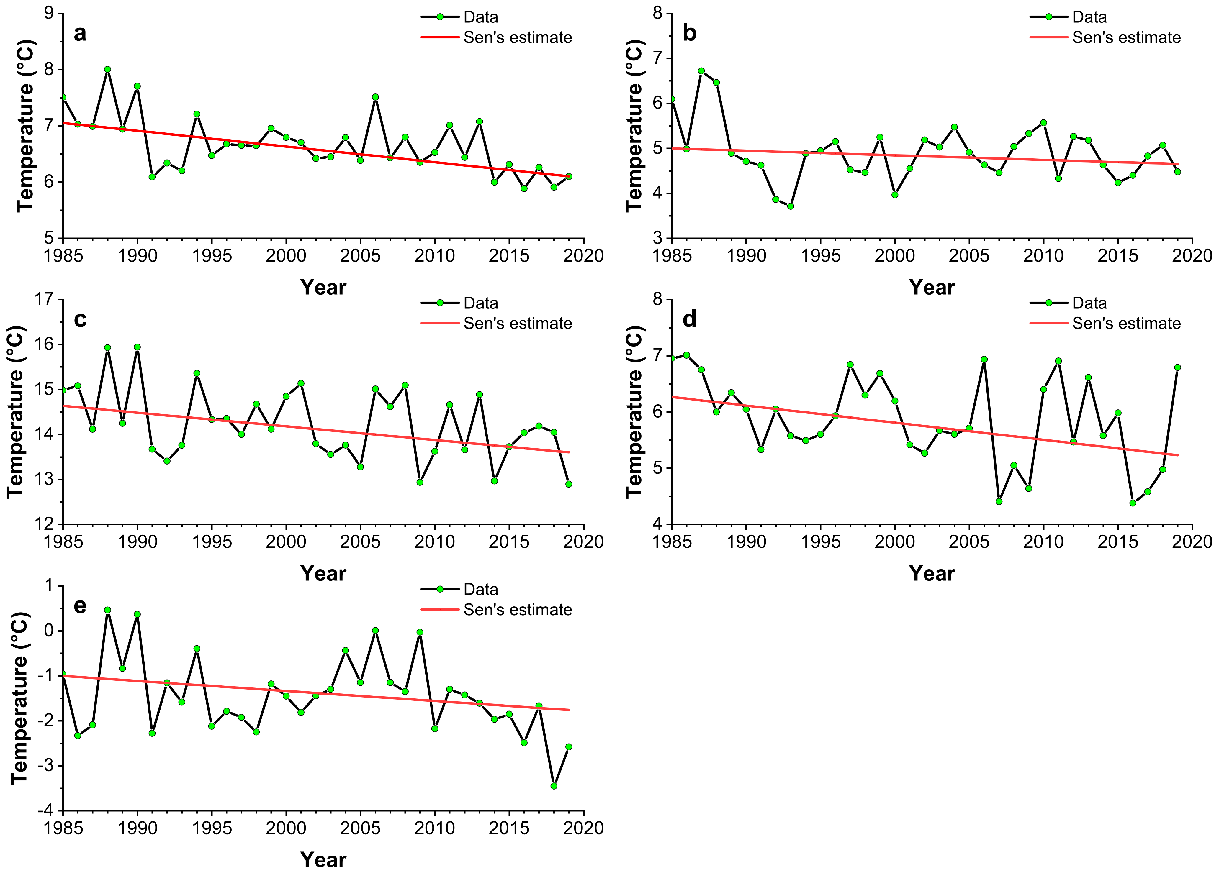
The mean annual minimum temperature shows a significant decrease at α = 0.01 level (Figure 3a), mean spring temperature shows a significant decrease at α = greater than 0.1 level (Figure 3b), mean summer and autumn temperature show a significant decrease at α = 0.05 level (Figure 3c,d) and mean winter temperature shows a significant decrease at α = greater than 0.1 level (Figure 3e) using Mann–Kendall. The statistical significance of the monthly, annual, and seasonal trends of the observed temperatures are given in Table 2. No positive trends were detected for monthly minimum temperature for the study area. For the all-monthly Mann–Kendall test, negative significance was detected for January, February, March, April, June, August, October, and November at α = greater than 0.1 level of significance, for September and December at α = 0.05 level of significance, and for May and July at α = 0.1 level of significance (Figure 4).

3.1.2. Monthly, Seasonal and Annual Maximum Trends for Temperature

The mean annual maximum temperature shows a significant increase at α = 0.1 level (Figure 5a), mean spring temperature shows a significant increase at α = greater than 0.05 level (Figure 5b), and mean summer, autumn, and winter temperature show a significant increase at α = greater than 0.1 level (Figure 5c–e) using Mann–Kendall. The statistical significance of the monthly, annual, and seasonal trends of the observed temperatures are given in Table 3. In this study, positive trends were detected for all monthly maximum temperatures for the study area except for June. For the all-monthly Mann–Kendall test, positive significance was detected for January, February, April, May, June, July, September, and November at α = greater than 0.1 level of significance, for March and October at α = 0.05 level of significance, and for August and December at α = 0.1 level of significance (Figure 6).

3.1.3. Monthly, Seasonal and Annual Trends for Precipitation

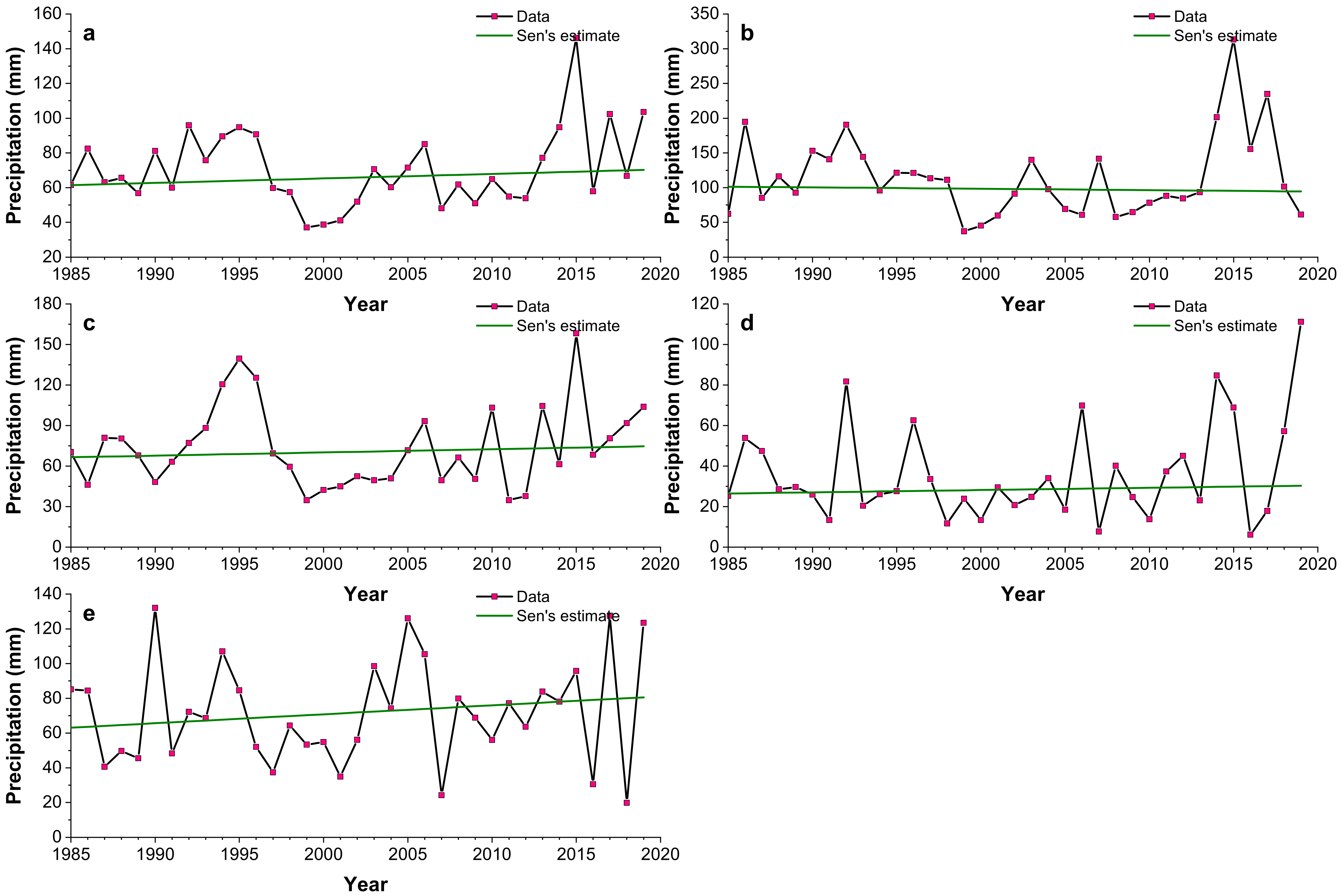
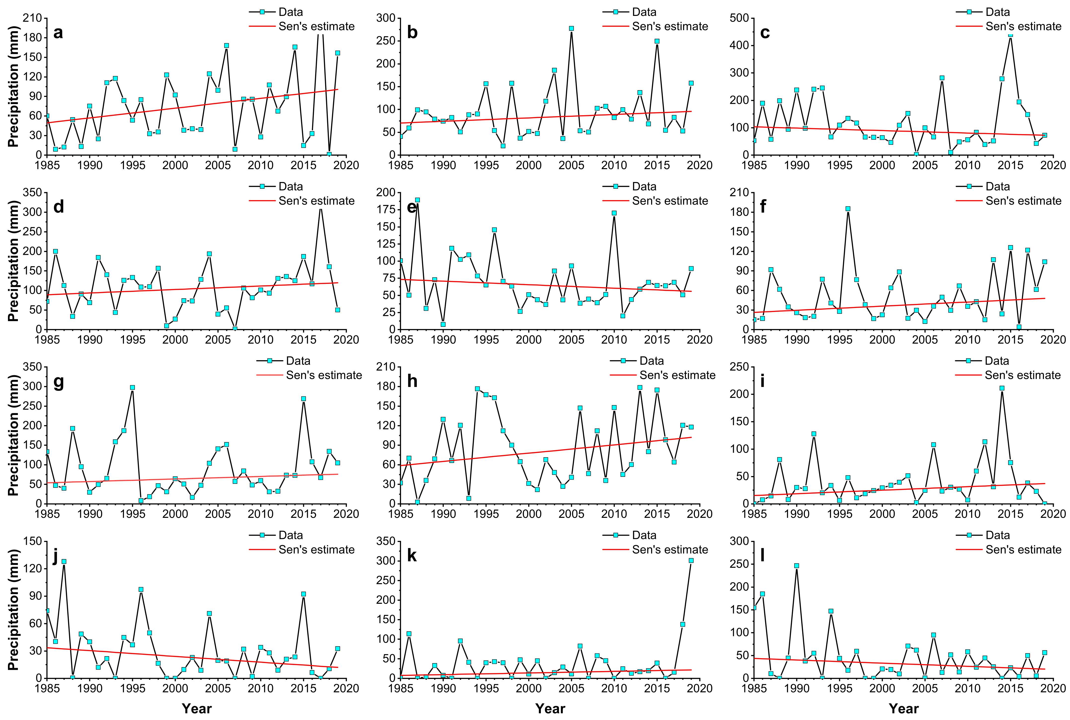
The Annual, Summer, Autumn, and Winter precipitation show a slightly significant increase. In spring, a slightly decreasing precipitation trend can be seen at α = greater than 0.01 level using Mann–Kendall (Table 4), as graphically represented in Figure 7. The statistical significance of the monthly, annual, and seasonal trends of the observed precipitation are given in Table 4. In this study, positive trends were detected for precipitation in January, February, April, June, July, August, September, and November for the study area, while no such trends were detected for March, May, October, and December at α = greater than 0.01 level using Mann–Kendall (Table 4), as graphically represented in Figure 8.

3.2. Snow Cover

In the given period, the snow-covered area changed to the non-snow-covered area after melting in various months. The average area of snow cover varied from 10% to 90%. The area had a maximum snow cover of 80–90% during the winter (December to February) season, and the least snow cover (10–15%) was observed in the summer (June to September) season. The computed snow cover is shown in Figure 9, which depicts snow cover distribution in the Lidder River watershed from 2010 to 2014. According to Figure 9, 2014 had the most snow (49% snow cover), while 2010 had the least (34% snow cover). The river discharge mainly depends on the change in a snow-covered area. When the snow cover data are compared with the observed streamflow data, the discharge is lowest in the winter season. As the mean temperature rises in April, the discharge rises, particularly in low elevation snow cover regions. The flow peaks in July, when glacial melt begins following the melting of new snow in the watershed.

3.3. Model Calibration

The catchment’s runoff due to snowmelt was modeled using SRM. Water losses are often relatively minor during the start of the snowmelt season, as the only outcome is evaporation from the snow cover. As the soil is uncovered and vegetation begins to develop, high water losses are predicted due to evapotranspiration and interception from the vegetation. First, the model was run without making any changes in the parameters for pre-calibration by using discharge data for the hydrological year 2009–2010, and the results were recorded. The SRM model performance at a daily scale was evaluated by plotting a graph between simulated and observed streamflows.
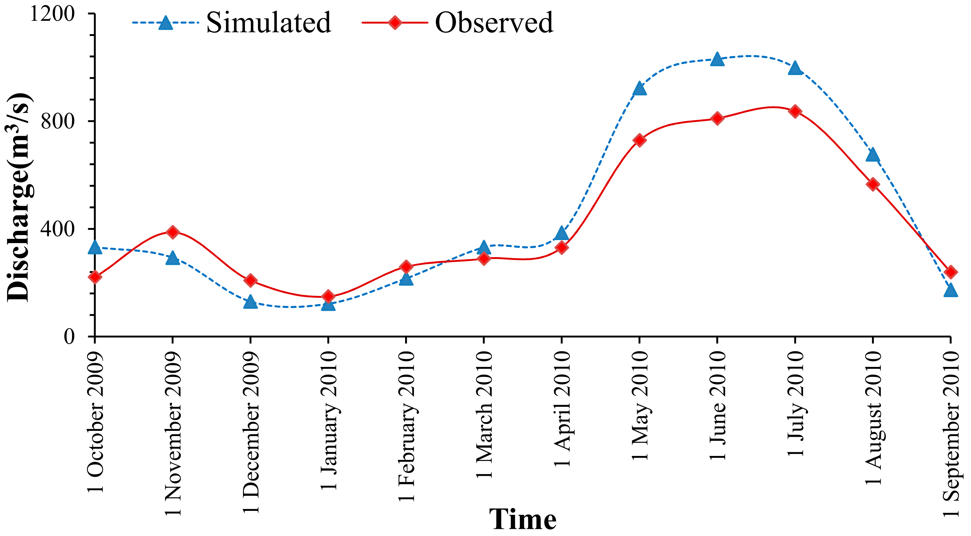
Furthermore, the model’s performance was assessed using the Dy and R2 values between simulated and observed streamflow. The simulated and observed discharge value in different months in pre-calibration is illustrated in Figure 10. It is evident from Figure 10 that the model mostly overestimated the discharge compared to the observed values in different months. It can be observed from Figure 10 that the model overestimated the runoff in the melting season. The simulated discharge values are higher and lower than those observed in different months. The R2 value was found to be 0.90 in the pre-calibration of the model. The highest value of discharge for pre-calibration is observed in June.
The calibration was conducted manually by running the SRM model numerous times for the 2009–2010 year, yielding an optimum value of the degree-day parameter for the watershed between 0.1- and 0.4-mm d−1 °C−1. After fine-tuning the model through numerous iterations, the optimal values for critical temperature, lag time, and recession coefficient were determined. The SRM model was calibrated for the 2009–2010 years. Figure 11 shows the calibrated results of simulated and observed runoff. According to Figure 11, the field observed and simulated discharges are matched well.
Furthermore, the maximum discharge during calibration was recorded in June. During calibration, the model’s accuracy requirements provide a volume difference (Dv) of 11.7% and an R2 value of 0.96. The simulation error indication indicates that the simulation is adequate for both daily and seasonal melting.

3.4. Model Validation

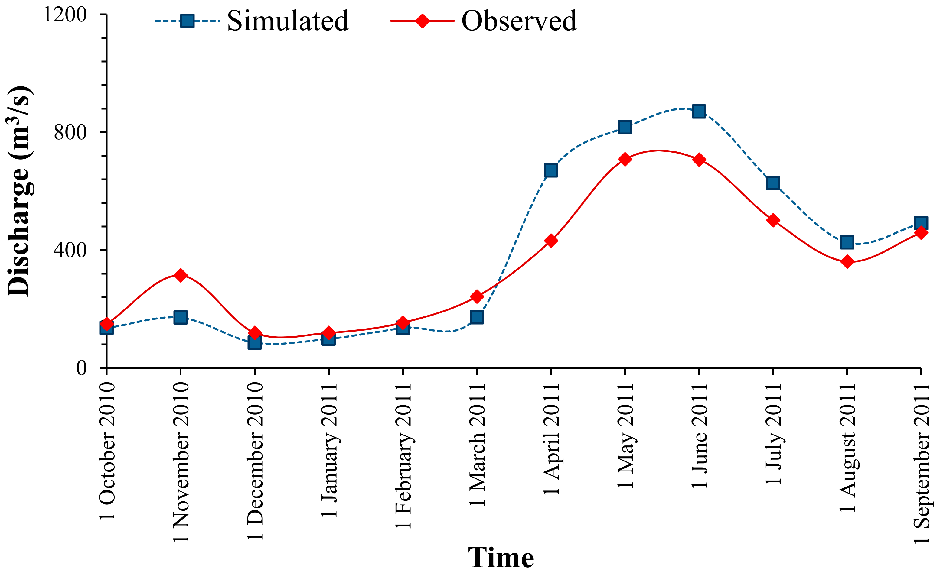
After calibrating the model, it could be transferred to another year by simply adjusting the input data while retaining the calibrated parameters. The model was validated for the hydrological years 2010–2011 to 2013–2014 yearly, with the same parameters used during calibration. The graphical representation between the simulated and observed discharge of the year 2010–2011 is given in Figure 12. It can be observed from Figure 12 that the simulated and the observed values for the discharge are in close agreement. It can be further observed that the highest value of discharge was found in June (869.8 m3/s). During the year 2010–2011, the performance indices were Dv = −10.1% and R2 = 0.92. The model slightly overestimated the discharge value; however, the difference is within reasonable limits. The model validation results show that the simulated and the observed values match well, with the statistical parameters within a reasonable range.
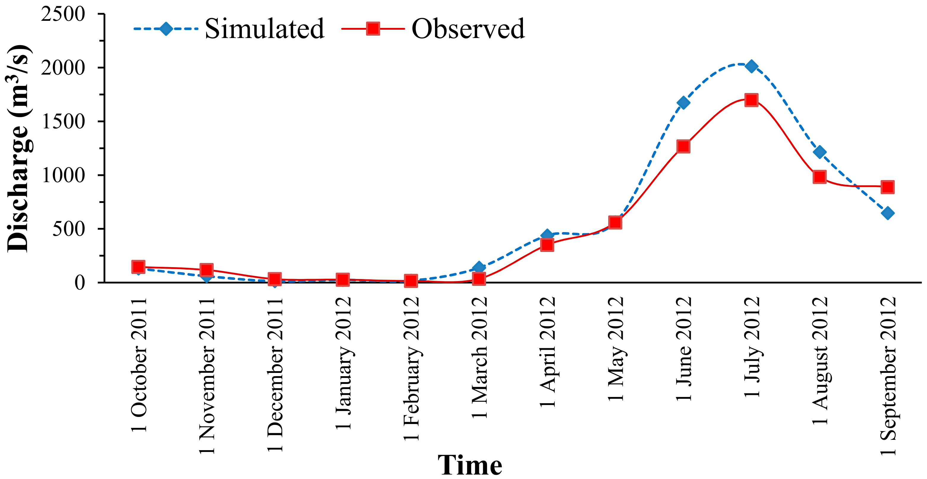
The model was run for the year 2011–2012 as well. The validation run shows the highest value of discharge in July. The graphical representation between modeled and field observed value of discharge is shown in Figure 13. The modeled and observed values were found in good agreement, with a Dv of −11.8% and R2 of 0.95. Similarly, the SRM model was run for 2012–2013 (Figure 14). It is evident from Figure 14 that the model performance was good, and the highest discharge value was found in July (1176.68 m3/s). The modeled and observed values agreed with the Dv value of 1.96% and R2value of 0.90. The simulated and observed values of 2013–2014 were plotted and had good agreement, with a Dv of 8.6% and R2 of 0.94 (Figure 15). The maximum discharge was observed in September of 2013–2014 (4381.57 m3/s), different from all the other years, because of excessive floods.
For 2009–2014, including calibration and validation, the yearly statistical error results indicate that the model performance is very good. However, it can be observed that the model overestimates and underestimates the streamflow at different times. The values were in high agreement compared to previous studies [49,55] conducted in the other regions of the world. The average value of R2 and Dv during the whole simulation period was 0.92% and 0.072%, respectively. The values of the statistical indicators are in a close range to those obtained during calibration and validation.
These findings imply that the SRM accuracy obtained in this work is excellent and may be used for runoff modeling in other Himalayan basins for water resource management and planning.

3.5. Climate Change Impact on Streamflow

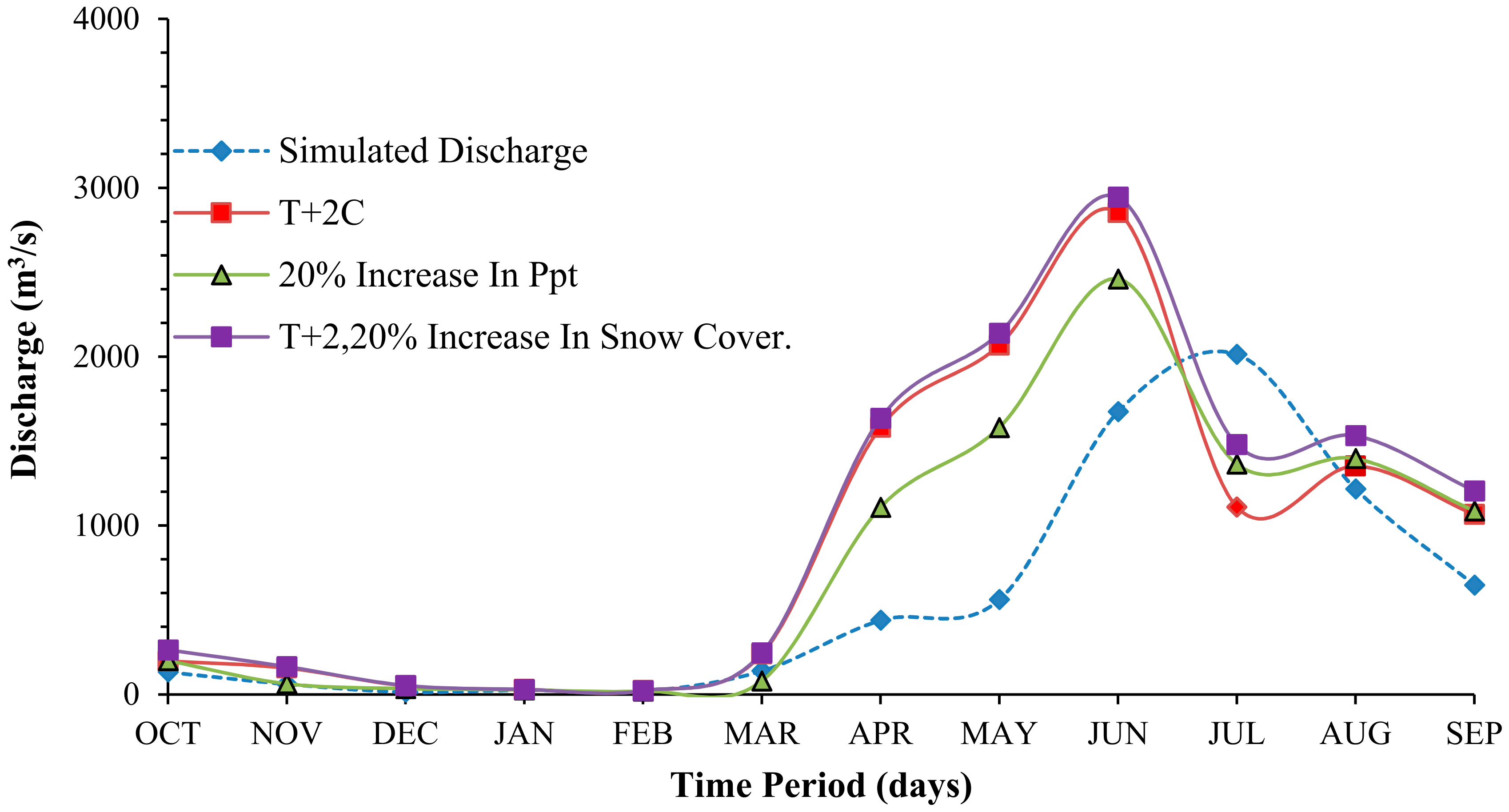
The impact of climate change under the three scenarios (mentioned in Section 2.7) was assessed using a simulation period of 2011–2012. The discharges simulated for each month of the hydrological year 2011–2012 under all scenarios are summarized in Table 2. Figure 10 depicts the discharge variation in all three scenarios.
In Scenario A, according to the findings, summer streamflow is predicted to rise as the snow cover area increases. If the mean temperature stays constant, a 20% increase in precipitation leads to an approximately 37% (2441 m3/s) increase in average discharge in summer (April-September) above the current average summer discharge (6553 m3/s) [39]. The peak discharge was the highest in July (2013.44 m3/s) in the simulated discharge values, with 2011–12 as the current year. In contrast, with the 20% change in precipitation, the peak discharge was shifted one month earlier to June (2460.11 m3/s).
In Scenario B, the results illustrated in Table 5 indicate that a 2 °C increase in temperature increased the average discharge 53% (3476 m3/s) in the summer. The peak discharge was highest in July (2013.44 m3/s). When the temperature changed by 2 °C, the peak discharge was shifted one month to June (2853.29 m3/s). This result indicates that if the rise in the air temperature continues at the rate of 3.7 °C [15], runoff must be carefully managed due to the large volumes of runoff received from the Lidder and its adjoining glacier and snowmelt regions.
The increase in temperature results in peak flow from June to July (Figure 16). If this scenario continues, the glaciers may recede significantly or perhaps even vanish after a time. Cannone et al. [56] reported on the fast melting of glaciers, explaining that the number of small glaciers (which cover 80% of the total area under glaciers and are essential for providing the water supply) might vanish in the coming decades due to the present warm climatic trend. These vanishing glaciers affect the hydrograph by changing the surface albedo and soil water storage capacity.
The discharge simulated under the condition of a 20% increase in snow cover and a 2% increase in mean temperature (Scenario C) resulted in a 67% increase in streamflow. The peak discharge was observed to be the highest in July (2013.44 m3/s) in the simulated discharge values with the year 2011–12 as the current year, whereas with an increase in temperature by 2 °C and increase in precipitation by 20%, the peak discharge was shifted by one month to June (2944.30 m3/s). These findings suggest that the discharge impacts the snow cover melt produced by the average temperature in summer. It is evident from Figure 16 that the streamflow increases with the variations in the hydro-meteorological parameters. The influence of the climate change studies indicates that catchment hydrology would be affected under climate change scenarios. This shift appears to be the effect of rising temperatures, which increase the streamflow in the region during summer. The snowmelt runoff appears to fluctuate in spring as precipitation and mean temperature rise, even though the climatic scenarios employed in this study give important information regarding how streamflow varies with temperature, precipitation, and snow cover.
According to Intergovernmental Panel on Climate Change (IPCC) predictions, future climate change brings a variety of repercussions. Figure 17 shows the precipitation changes in the Lidder river watershed under the A2 and B2 scenarios from the year 2020 to 2080. It is indicated that the future annual precipitation in the Lidder river catchment is decreasing. From the A2 and B2 scenarios, it is evident that the monthly precipitation decreases throughout spring, summer, and fall, then has a rising tendency during the winter. Figure 18 depicts the average changes in mean temperature in both scenarios from 2020 to 2080. There is a growing trend in the future mean temperature seasonal. The increasing range under A2 is greater than B2. A similar result was observed in Ungauged Mountainous Watershed, Northwest China, by Ma et al. [57]; in Alberta, Canada, by Jiang et al. [58]; and in the Sutlej River Basin, India, by Singh et al. [59].
In this investigation, 2010–11 is used as a reference year for the above climate scenarios. In 2020, the mean precipitation was predicted to decline in spring and summer by 1.2% and 3.8%, respectively. At the same time, mean watershed temperatures were predicted to climb 1.5 °C in both seasons. In 2050, average precipitation was predicted to decline in spring and summer at 0.3% and 4.8%, respectively. At the same time, the average temperature of the catchment was predicted to climb in spring and summer as 1.8 °C and 2.2 °C, respectively. In the 2080s, average precipitation in spring and summer is declined by 1.7% and 12.1%, respectively. At the same time, average catchment temperatures were predicted to climb 3.1 °C and 3.4 °C, respectively. These results show that streamflow in the spring is expected to increase with increasing mean temperature, whereas streamflow in the summer declines with decreasing precipitation. The average streamflow during the summer is down 4.3% in the 2020s and up 1.5% and 10.1% in the 2050s and 2080s, respectively. The findings further suggest that as the snow cover area increases, streamflow will increase in the spring and summer. The mean discharge increases by 12.6% during the snowmelt seasons due to the increase in snow cover percentage (i.e., 20%).

4. Conclusions

Snow cover research is critical for climatological and hydrological studies. The daily temperature, snow cover, and precipitation were chosen as input data to simulate snowmelt runoff using the SRM model. The simulated and observed runoff values were evaluated using an SRM model of the Lidder catchment. The SRM model results provided an R2 value of 0.96, 0.92, 0.95, 0.90, and 0.94, respectively, for 2009–2014 during the calibration and validation period, while the Dv for the same years was found to be 11.7, −10.1, −11.8, 1.96 and 8.6, respectively. The average R2 value for all simulated years was 0.93, and the average Dv value was 0.072%. The simulated monthly discharge was in close agreement with the observed values in the calibration and validation periods. According to a climatic scenario, a 20% rise in precipitation could increase the runoff by as much as 37%. A temperature increase of 2 °C resulted in a 53% rise in catchment discharge and a 20% rise in snow cover. With a temperature increase of 2 °C and an increase in snow cover by 20%, the peak discharge was shifted by one month, from July to June. The flow rate was 2944.30 m3/s compared to the peak discharge observed in July (2013.44 m3/s). The SRM model shows that the influence of climate change on precipitation and temperature, and thereby on runoff, is considerable. With increasing snow cover area, spring and summer streamflow is projected to rise. A 20% increase in snow cover causes the average streamflow during the snowmelt seasons to rise by 12.6%. These results reveal that the SRM model is the best method for quantifying runoff due to snowmelt and numerous processes linked to hydrology, climate, and ecology in mountainous and ungauged places.

Author Contributions

Conceptualization, S.M. and R.K.; methodology, R.K.; software, K.S.; validation, K.S., R.K. and D.K.V.; formal analysis, S.M.; investigation, R.K.; resources, R.K.; data curation, S.M.; writing—original draft preparation, S.M. and D.K.V.; writing—review and editing, R.K., N.L.K., S.M., A.K. and A.E.; visualization, S.M., D.K.V. and V.P.; supervision, R.K.; project administration, R.K.; funding acquisition, N.A.-A. All authors have read and agreed to the published version of the manuscript.

Funding

This research received no external funding.

Data Availability Statement

Not applicable.

Acknowledgments

The authors are highly thankful to the College of Agricultural Engineering and Technology, Sher-e-Kashmir University of Agricultural Sciences and Technology of Kashmir, Shalimar Campus Srinagar-190025 for providing all necessary facilities to conduct this study. The authors gratefully acknowledge the critical reviews of anonymous reviewers and the editor, which improved the manuscript significantly. Alban Kuriqi acknowledges the Portuguese Foundation for Science and Technology (FCT) support through PTDC/CTA-OHR/30561/2017 (WinTherface).

Conflicts of Interest

The authors declare no conflict of interest.

References

  1. Jeelani, G.; Bhat, N.A.; Shivanna, K. Use of δ18O tracer to identify stream and spring origins of a mountainous catchment: A case study from Liddar watershed, Western Himalaya, India. J. Hydrol. 2010, 393, 257–264. [Google Scholar] [CrossRef]
  2. Jeelani, G.; Feddema, J.J.; van der Veen, C.J.; Stearns, L. Role of snow and glacier melt in controlling river hydrology in Liddar watershed (western Himalaya) under current and future climate. Water Resour. Res. 2012, 48, 1–16. [Google Scholar] [CrossRef] [Green Version]
  3. Aggarwal, S.P.; Thakur, P.K.; Nikam, B.R.; Garg, V. Integrated approach for snowmelt runoff estimation using temperature index model, remote sensing and GIS. Curr. Sci. 2014, 106, 397–407. [Google Scholar] [CrossRef]
  4. Kushwaha, N.L.; Bhardwaj, A. Hydrologic response of Takarla-Ballowal watershed in Shivalik foot-hills based on morphometric analysis using Remote Sensing and GIS. Indian Water Resour. Soc. 2016, 36, 17–25. [Google Scholar]
  5. Jain, S.K.; Goswami, A.; Saraf, A.K. Snowmelt runoff modelling in a Himalayan basin with the aid of satellite data. Int. J. Remote Sens. 2010, 31, 6603–6618. [Google Scholar] [CrossRef]
  6. Naser, S. Modelling and isotopic studies for assessment of contribution of snow/glacier melt in Parvati Basin, Himachal Pradesh. Am. J. Geol. Ecol 2013, 3, 2568–5449. [Google Scholar]
  7. Mote, P.W.; Hamlet, A.F.; Clark, M.P.; Lettenmaier, D.P. Declining Mountain Snowpack in Western North America. Bull. Am. Meteorol. Soc. 2005, 86, 39–50. [Google Scholar] [CrossRef]
  8. Stewart, I.T. Changes in snowpack and snowmelt runoff for key mountain regions. Hydrol. Process. 2009, 23, 78–94. [Google Scholar] [CrossRef]
  9. Knowles, N.; Dettinger, M.D.; Cayan, D.R. Trends in Snowfall versus Rainfall in the Western United States. J. Clim. 2006, 19, 4545–4559. [Google Scholar] [CrossRef] [Green Version]
  10. Ahluwalia, R.S.; Rai, S.P.; Jain, S.K.; Kumar, B.; Dobhal, D.P. Assessment of snowmelt runoff modelling and isotope analysis: A case study from the western Himalaya, India. Ann. Glaciol. 2013, 54, 299–304. [Google Scholar] [CrossRef] [Green Version]
  11. Rood, S.B.; Pan, J.; Gill, K.M.; Franks, C.G.; Samuelson, G.M.; Shepherd, A. Declining summer flows of Rocky Mountain rivers: Changing seasonal hydrology and probable impacts on floodplain forests. J. Hydrol. 2008, 349, 397–410. [Google Scholar] [CrossRef]
  12. Maurer, E.P.; Rhoads, J.D.; Dubayah, R.O.; Lettenmaier, D.P. Evaluation of the snow-covered area data product from MODIS. Hydrol. Process. 2003, 17, 59–71. [Google Scholar] [CrossRef]
  13. Shekhar, M.S.; Chand, H.; Kumar, S.; Srinivasan, K.; Ganju, A. Climate-change studies in the western Himalaya. Ann. Glaciol. 2010, 51, 105–112. [Google Scholar] [CrossRef] [Green Version]
  14. Bhutiyani, M.R.; Kale, V.S.; Pawar, N.J. Changing streamflow patterns in the rivers of northwestern Himalaya: Implications of global warming in the 20th century. Curr. Sci. 2008, 95, 618–626. [Google Scholar]
  15. IPCC. Climate Change 2014: Synthesis report. In Contribution of Working Groups I, II and III to the Fifth Assessment Report of the Intergovernmental Panel on Climate Change; Pachauri, R.K., Allen, M.R., Barros, V.R., Broome, J., Cramer, W., Christ, R., Church, J.A., Clarke, L., Dahe, Q., Dasgupta, P., Eds.; IPCC: Geneva, Switzerland, 2014; p. 151. ISBN 9291691437. [Google Scholar]
  16. Wang, S.; Zhang, T. Glacial lakes change and current status in the central Chinese Himalayas from 1990 to 2010. J. Appl. Remote Sens. 2013, 7, 073459. [Google Scholar] [CrossRef]
  17. Tekeli, A.E.; Akyürek, Z.; Arda Şorman, A.; Şensoy, A.; Ünal Şorman, A. Using MODIS snow cover maps in modeling snowmelt runoff process in the eastern part of Turkey. Remote Sens. Environ. 2005, 97, 216–230. [Google Scholar] [CrossRef]
  18. Romshoo, S.A.; Rafiq, M.; Rashid, I. Spatio-temporal variation of land surface temperature and temperature lapse rate over mountainous Kashmir Himalaya. J. Mt. Sci. 2018, 15, 563–576. [Google Scholar] [CrossRef]
  19. Bales, R.C.; Molotch, N.P.; Painter, T.H.; Dettinger, M.D.; Rice, R.; Dozier, J. Mountain hydrology of the western United States. Water Resour. Res. 2006, 42. [Google Scholar] [CrossRef]
  20. Wagener, T.; Wheater, H.; Gupta, H.V. Rainfall-Runoff Modelling in Gauged and Ungauged Catchments; World Scientific: London, UK, 2004; ISBN 1860944663. [Google Scholar]
  21. Tanmoyee, B.; V, R.P.; Abdul, H. Climate Change Impact on Snowmelt Runoff Modelling for Alaknanda River Basin. J. Environ. Earth Sci. 2015, 5, 139–150. [Google Scholar]
  22. Singh, V.P.; Woolhiser, D.A. Mathematical Modeling of Watershed Hydrology. J. Hydrol. Eng. 2002, 7, 270–292. [Google Scholar] [CrossRef] [Green Version]
  23. Wheater, H.S. Modelling hydrological processes in arid and semi-arid areas: An introduction to the workshop. Hydrol. Model. Arid. Semi-Arid Areas 2008, 1–20. [Google Scholar] [CrossRef]
  24. Martinec, J.; Rango, A.; Roberts, R. Snowmelt Runoff Model (SRM) User’s Manual: Updated Edition for Windows (WinSRM Version 1.11); New Mexico State University: Las Cruces, Mexico, 2007. [Google Scholar]
  25. Javadinejad, S.; Dara, R.; Jafary, F. Climate change scenarios and effects on snowmelt runoff. Civ. Eng. J. 2020, 6, 1715–1725. [Google Scholar] [CrossRef]
  26. Fuladipanah, M.; Jorabloo, M. The estimation of snowmelt runoff using SRM case study (Gharasoo Basin, Iran). World Appl. Sci. J. 2012, 17, 433–438. [Google Scholar]
  27. Kaul, M.N. Glacial and Fluvial Geomorphology of Western Himalaya: Liddar Valley; Concept Publishing Company: New Delhi, India, 1990; ISBN 8170222443. [Google Scholar]
  28. Malik, M.I.; Bhat, M.S. Integrated Approach for Prioritizing Watersheds for Management: A Study of Lidder Catchment of Kashmir Himalayas. Environ. Manage. 2014, 54, 1267–1287. [Google Scholar] [CrossRef] [PubMed]
  29. Ma, H.; Cheng, G. A test of Snowmelt Runoff Model (SRM) for the Gongnaisi River basin in the western Tianshan Mountains, China. Chin. Sci. Bull. 2003, 48, 2253–2259. [Google Scholar] [CrossRef]
  30. Yu, M.; Chen, X.; Li, L.; Bao, A.; de la Paix, M.J. Incorporating accumulated temperature and algorithm of snow cover calculation into the snowmelt runoff model. Hydrol. Process. 2013, 27, 3589–3595. [Google Scholar] [CrossRef]
  31. Immerzeel, W.W.; Droogers, P.; de Jong, S.M.; Bierkens, M.F.P. Large-scale monitoring of snow cover and runoff simulation in Himalayan river basins using remote sensing. Remote Sens. Environ. 2009, 113, 40–49. [Google Scholar] [CrossRef]
  32. Tahir, A.A.; Chevallier, P.; Arnaud, Y.; Neppel, L.; Ahmad, B. Modeling snowmelt-runoff under climate scenarios in the Hunza River basin, Karakoram Range, Northern Pakistan. J. Hydrol. 2011, 409, 104–117. [Google Scholar] [CrossRef]
  33. Georgievsky, M. V Application of the Snowmelt Runoff model in the Kuban river basin using MODIS satellite images. Environ. Res. Lett. 2009, 4, 45017. [Google Scholar] [CrossRef] [Green Version]
  34. Harshburger, B.J.; Walden, V.P.; Humes, K.S.; Moore, B.C.; Blandford, T.R.; Rango, A. Generation of Ensemble Streamflow Forecasts Using an Enhanced Version of the Snowmelt Runoff Model1. JAWRA J. Am. Water Resour. Assoc. 2012, 48, 643–655. [Google Scholar] [CrossRef]
  35. Rasouli, H.; Kayastha, R.B.; Bhattarai, B.C.; Shrestha, A.; Arian, H.; Armstrong, R. Estimation of Discharge From Upper Kabul River Basin, Afghanistan Using the Snowmelt Runoff Model. J. Hydrol. Meteorol. 2016, 9, 85–94. [Google Scholar] [CrossRef] [Green Version]
  36. Vafakhah, M.; Nouri, A.; Alavipanah, S.K. Snowmelt-runoff estimation using radiation SRM model in Taleghan watershed. Environ. Earth Sci. 2015, 73, 993–1003. [Google Scholar] [CrossRef]
  37. Senzeba, K.T.; Bhadra, A.; Bandyopadhyay, A. Snowmelt runoff modelling in data scarce Nuranang catchment of eastern Himalayan region. Remote Sens. Appl. Soc. Environ. 2015, 1, 20–35. [Google Scholar] [CrossRef]
  38. Gurung, A.; Kayastha, R.B.; Shrestha, A. Estimation of Discharge of Langtang River, Nepal using Snowmelt Runoff Model. In Participatory Community Assessment for Priority Problem Diagnosis in Bajura District, Nepal: What Matters Most–Poverty or Climate Change? Utah State University: Logan, UT, USA, 2015; pp. 199–204. Available online: https://www.researchgate.net/profile/Lam-Ya-Mostaque/publication/328575672_Climate_Change_Induced_Migration_Impact_on_'Slumaisation'/links/5d7a0bf74585151ee4af7794/Climate-Change-Induced-Migration-Impact-on-Slumaisation.pdf#page=213 (accessed on 12 September 2021).
  39. Xie, S.; Du, J.; Zhou, X.; Zhang, X.; Feng, X.; Zheng, W.; Li, Z.; Xu, C.-Y. A progressive segmented optimization algorithm for calibrating time-variant parameters of the snowmelt runoff model (SRM). J. Hydrol. 2018, 566, 470–483. [Google Scholar] [CrossRef]
  40. Hayat, H.; Akbar, T.A.; Tahir, A.A.; Hassan, Q.K.; Dewan, A.; Irshad, M. Simulating Current and Future River-Flows in the Karakoram and Himalayan Regions of Pakistan Using Snowmelt-Runoff Model and RCP Scenarios. Water 2019, 11, 761. [Google Scholar] [CrossRef] [Green Version]
  41. Xiang, Y.; Li, L.; Chen, J.; Xu, C.-Y.; Xia, J.; Chen, H.; Liu, J. Parameter Uncertainty of a Snowmelt Runoff Model and Its Impact on Future Projections of Snowmelt Runoff in a Data-Scarce Deglaciating River Basin. Water 2019, 11, 2417. [Google Scholar] [CrossRef] [Green Version]
  42. Karimi, H.; Zeinivand, H.; Tahmasebipour, N.; Haghizadeh, A.; Miryaghoubzadeh, M. Comparison of SRM and WetSpa models efficiency for snowmelt runoff simulation. Environ. Earth Sci. 2016, 75, 1–16. [Google Scholar] [CrossRef]
  43. Nourani, V.; Afkhaminia, A.; Andaryani, S.; Zhang, Y. Multi-station calibration strategy for evaluation and sensitivity analysis of the snowmelt runoff model using MODIS satellite images. Hydrol. Res. 2021, 52, 1389–1404. [Google Scholar] [CrossRef]
  44. Siemens, K.; Dibike, Y.; Shrestha, R.R.; Prowse, T. Runoff Projection from an Alpine Watershed in Western Canada: Application of a Snowmelt Runoff Model. Water 2021, 13, 1199. [Google Scholar] [CrossRef]
  45. Yi, Y.; Liu, S.; Zhu, Y.; Wu, K.; Xie, F.; Saifullah, M. Spatiotemporal heterogeneity of snow cover in the central and western Karakoram Mountains based on a refined MODIS product during 2002–2018. Atmos. Res. 2021, 250, 105402. [Google Scholar] [CrossRef]
  46. Bolch, T.; Kulkarni, A.; Kääb, A.; Huggel, C.; Paul, F.; Cogley, J.G.; Frey, H.; Kargel, J.S.; Fujita, K.; Scheel, M.; et al. The State and Fate of Himalayan Glaciers. Science 2012, 336, 310–314. [Google Scholar] [CrossRef] [PubMed] [Green Version]
  47. Scherler, D.; Bookhagen, B.; Strecker, M.R. Spatially variable response of Himalayan glaciers to climate change affected by debris cover. Nat. Geosci. 2011, 4, 156–159. [Google Scholar] [CrossRef]
  48. Martinec, J. Snowmelt-runoff model for stream flow forecasts. Hydrol. Res. 1975, 6, 145–154. [Google Scholar] [CrossRef]
  49. Butt, M.J.; Bilal, M. Application of snowmelt runoff model for water resource management. Hydrol. Process. 2011, 25, 3735–3747. [Google Scholar] [CrossRef]
  50. Li, X.; Williams, M.W. Snowmelt runoff modelling in an arid mountain watershed, Tarim Basin, China. Hydrol. Process. 2008, 22, 3931–3940. [Google Scholar] [CrossRef]
  51. Kushwaha, N.L.; Rajput, J.; Elbeltagi, A.; Elnaggar, A.Y.; Sena, D.R.; Vishwakarma, D.K.; Mani, I.; Hussein, E.E. Data Intelligence Model and Meta-Heuristic Algorithms-Based Pan Evaporation Modelling in Two Different Agro-Climatic Zones: A Case Study from Northern India. Atmosphere 2021, 12, 1654. [Google Scholar] [CrossRef]
  52. Vishwakarma, D.K.; Pandey, K.; Kaur, A.; Kushwaha, N.L.; Kumar, R.; Ali, R.; Elbeltagi, A.; Kuriqi, A. Methods to estimate evapotranspiration in humid and subtropical climate conditions. Agric. Water Manag. 2022, 261, 107378. [Google Scholar] [CrossRef]
  53. Modeling of Stage-Discharge Using Back Propagation ANN-, ANFIS-, and WANN-based Computing Techniques. Available online: https://assets.researchsquare.com/files/rs-696059/v1_covered.pdf?c=1637668418 (accessed on 12 September 2021).
  54. Singh, P.; Kumar, N. Effect of orography on precipitation in the western Himalayan region. J. Hydrol. 1997, 199, 183–206. [Google Scholar] [CrossRef]
  55. Prasad, V.H.; Roy, P.S. Estimation of Snowmelt Runoff in Beas Basin, India. Geocarto Int. 2005, 20, 41–47. [Google Scholar] [CrossRef]
  56. Cannone, N.; Wagner, D.; Hubberten, H.W.; Guglielmin, M. Biotic and abiotic factors influencing soil properties across a latitudinal gradient in Victoria Land, Antarctica. Geoderma 2008, 144, 50–65. [Google Scholar] [CrossRef] [Green Version]
  57. Ma, Y.; Huang, Y.; Chen, X.; Li, Y.; Bao, A. Modelling Snowmelt Runoff under Climate Change Scenarios in an Ungauged Mountainous Watershed, Northwest China. Math. Probl. Eng. 2013, 2013, 808565. [Google Scholar] [CrossRef] [Green Version]
  58. Jiang, R.; Gan, T.Y.; Xie, J.; Wang, N.; Kuo, C.C. Historical and potential changes of precipitation and temperature of Alberta subjected to climate change impact: 1900–2100. Theor. Appl. Climatol. 2017, 127, 725–739. [Google Scholar] [CrossRef]
  59. Singh, D.; Jain, S.K.; Gupta, R.D. Statistical downscaling and projection of future temperature and precipitation change in middle catchment of Sutlej River Basin, India. J. Earth Syst. Sci. 2015, 124, 843–860. [Google Scholar] [CrossRef]
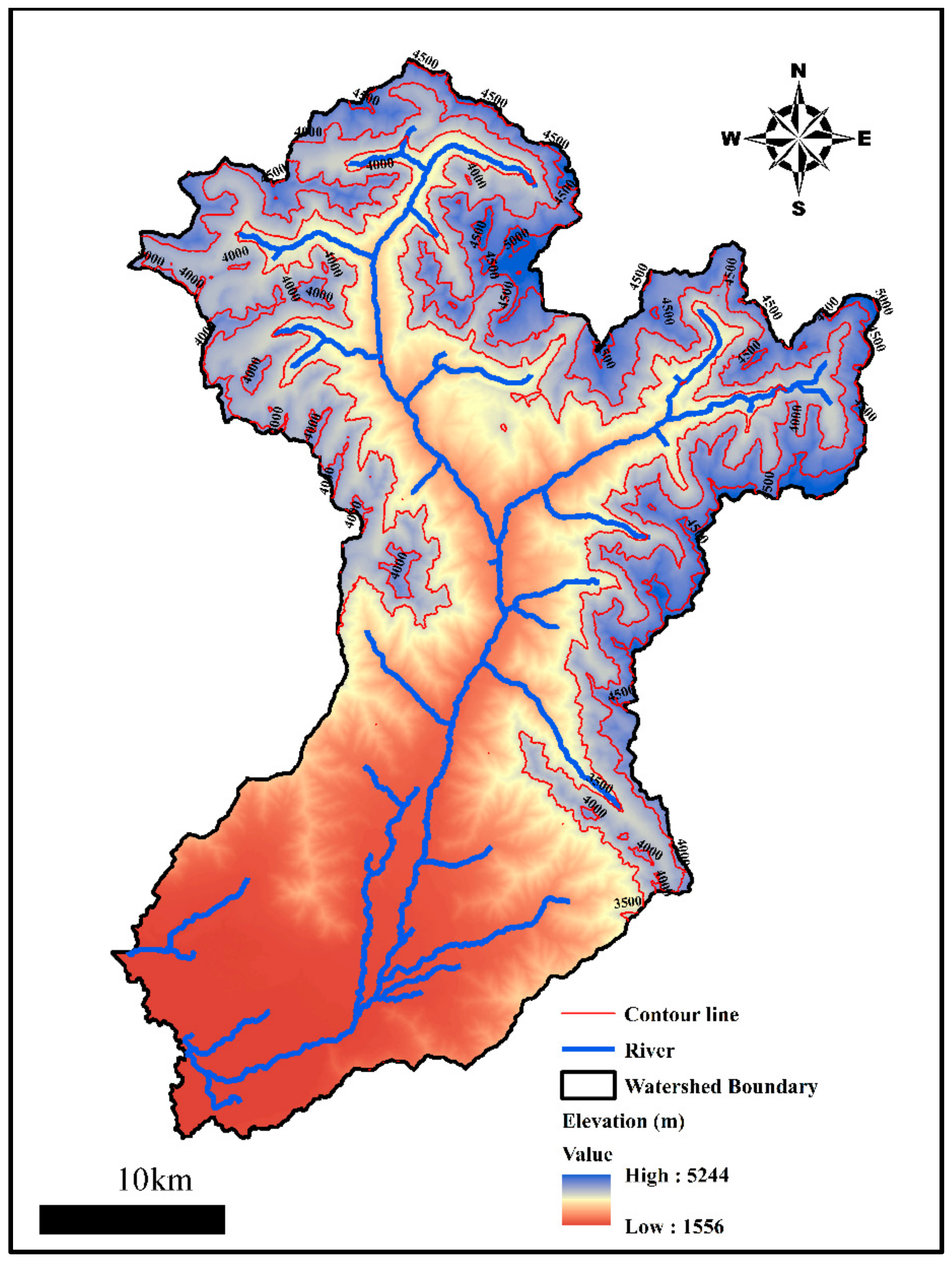
Figure 1. Location map of the study area located in the Lidder watershed (Pahalgan, Jammu, and Kashmir); the elevation of the meteorological station is 2196 MSL. The DEM contour lines correspond to the maximum and minimum extension of snow as of 20 December 2021.
Sustainability 14 01150 g001
Figure 2. Monthly variations in (a) Precipitation and (b) Temperature of Lidder basin during 2009–2014.
Sustainability 14 01150 g002aSustainability 14 01150 g002b
Figure 3. Trend statistics and Sen’s slope in observed seasonal minimum temperatures at study area from 1985 to 2019. (a) Average annual minimum temperature, (b) Average spring minimum temperature, (c) Average summer minimum temperature, (d) Average autumn minimum temperature, (e) Average winter minimum temperature.
Sustainability 14 01150 g003
Figure 4. Trend statistics and Sen’s slope observed monthly minimum temperatures in the study area from 1985 to 2019. (a) January, (b) February, (c) March, (d) April, (e) May, (f) June, (g) July, (h) August, (i) September, (j) October, (k) November, (l) December.
Sustainability 14 01150 g004
Figure 5. Trend statistics and Sen’s slope in observed seasonal maximum temperatures in the study area from 1985 to 2019. (a) Average annual minimum temperature, (b) Average spring minimum temperature, (c) Average summer minimum temperature, (d) Average autumn minimum temperature, (e) Average winter minimum temperature.
Sustainability 14 01150 g005
Figure 6. Trend statistics and Sen’s slope observed monthly maximum temperatures in the study area from 1985 to 2019. (a) January, (b) February, (c) March, (d) April, (e) May, (f) June, (g) July, (h) August, (i) September, (j) October, (k) November, (l) December.
Sustainability 14 01150 g006
Figure 7. Trend statistics and Sen’s slope in observed seasonal precipitation in the study area from 1985 to 2019. (a) Average annual maximum temperature, (b) Average spring maximum temperature, (c) Average summer maximum temperature, (d) Average autumn maximum temperature, (e) Average winter maximum temperature.
Sustainability 14 01150 g007
Figure 8. Trend statistics and Sen’s slope observed monthly precipitation in the study area from 1985 to 2019. (a) January, (b) February, (c) March, (d) April, (e) May, (f) June, (g) July, (h) August, (i) September, (j) October, (k) November, (l) December.
Sustainability 14 01150 g008
Figure 9. Snow cover distribution in the Lidder basin.
Sustainability 14 01150 g009
Figure 10. Simulated and observed discharge in different months for the basin’s the hydrological year 2009–2010 (pre-calibration).
Sustainability 14 01150 g010
Figure 11. On calibration, the model’s simulated and observed discharge in different months of the hydrological Year 2009–2010 in the Lidder basin.
Sustainability 14 01150 g011
Figure 12. On validation, the model’s simulated and observed discharge in different months of the hydrological Year 2010–2011 in the Lidder basin.
Sustainability 14 01150 g012
Figure 13. On validation, the model’s simulated and observed discharge in different months of the hydrological Year 2011–2012 in the Lidder basin.
Sustainability 14 01150 g013
Figure 14. On validation, the model’s simulated and observed discharge in different months of the hydrological Year 2012–2013 in the Lidder basin.
Sustainability 14 01150 g014
Figure 15. On validation, the model’s simulated and observed discharge in different months of the hydrological Year 2013–2014 in the Lidder basin.
Sustainability 14 01150 g015
Figure 16. Climate change run of SRM with temperature, precipitation, and discharge changes.
Sustainability 14 01150 g016
Figure 17. Precipitation changes in IPCC SERS A2 and B2 scenarios from the 2020s through the 2080s.
Sustainability 14 01150 g017
Figure 18. Temperature changes under IPCC SERS A2 and B2 scenarios from the 2020s through the 2080s.
Sustainability 14 01150 g018
Table 1. SRM model final input parameter values.
ParametersValues
Degree-day factor0.5
Runoff coefficient (rain)0.1–0.4
Runoff coefficient (snow)0.1–0.4 (October–February)
0.5–0.7 (March–September)
Temperature lapse rate (°C/100 m)0.44
Critical Temperature (°C)0.8
Lag Time (hours)
Recession Coefficient18
X-Coefficient1.03 and 1.04
Y-Coefficient0.01 and 0.03
Table 2. Z Mann–Kendall test statistics for annual, seasonal, and monthly minimum temperatures.
Time SeriesMann–Kendall Trend Statistics
Test ZSignificance LevelSen’s Slope Estimate
January−0.568 −0.018
February−0.511 −0.010
March−1.051 −0.019
April−0.682 −0.008
May−1.818+−0.035
June−1.463 −0.037
July−1.647+−0.033
August−1.221 −0.023
September−2.414*−0.039
October−1.108 −0.031
November−0.795 −0.015
December−2.429*−0.068
Annual−3.210**−0.028
Spring−0.852 −0.010
Summer−2.159*−0.030
Autumn−2.159*−0.030
Winter−1.619 −0.022
Table 3. Z statistic of Mann–Kendall test for annual, seasonal, and monthly maximum temperature.
Time SeriesMann–Kendall Trend Statistics
Test ZSignificance LevelSen’s Slope Estimate
January1.392 0.085
February0.483 0.013
March2.386*0.089
April0.966 0.027
May1.023 0.041
June−0.341 −0.008
July1.591 0.035
August1.846+0.034
September0.312 0.011
October1.974*0.066
November−0.852 −0.028
December1.818+0.042
Annual1.960+0.033
Spring2.215*0.058
Summer1.562 0.024
Autumn0.738 0.015
Winter1.591 0.055
Table 4. Z statistic of Mann–Kendall test for annual, seasonal, and monthly precipitation.
Time SeriesMann–Kendall Trend Statistics
Test ZSignificance LevelSen’s Slope Estimate
January1.591 1.504
February1.179 0.748
March−0.880 −0.900
April0.852 0.894
May−0.852 −0.509
June1.179 0.630
July0.937 0.648
August1.221 1.272
September1.363 0.642
October−1.536 −0.633
November0.944 0.415
December−0.939 −0.691
Annual0.596 0.258
Spring−0.256 −0.200
Summer0.568 0.238
Autumn0.284 0.113
Winter0.738 0.515
Table 5. Climate change run of SRM with precipitation, temperature, and snow cover changes.
Climate Change
Run
Simulated Discharge
of 2011–2012
(m3/s)
Simulated Discharge (m3/s)
With 20% Increase in PrecipitationWith Temperature +2 °CWith Temperature +2 °C and 20% Snow Cover
October132.52199.34197.72263.52
November61.3362.82156.03164.27
December14.4834.8250.8653.08
January26.0926.6229.4429.44
February19.1619.5521.7121.71
March139.2579.27239.42245.61
April439.551107.841581.141635.27
May562.031580.132067.092138.59
June1674.452460.112853.292944.30
July2013.441363.841110.061479.76
August1216.131396.281351.771531.65
September647.411086.181065.631205.03
Publisher’s Note: MDPI stays neutral with regard to jurisdictional claims in published maps and institutional affiliations.