Article

Trends in College–High School Wage Differentials in China: The Role of Cohort-Specific Labor Supply Shift

Business School, Beijing Normal University, Beijing 100875, China
Sustainability 2022, 14(24), 16917; https://doi.org/10.3390/su142416917
Submission received: 11 October 2022 / Revised: 5 December 2022 / Accepted: 14 December 2022 / Published: 16 December 2022
(This article belongs to the Special Issue Labor Economics and Sustainability)

Abstract

:
The wage gap between 4-year college (BA) and high school (HS) graduates narrows down among young workers from 2002 to 2009 in urban China, despite steadily increasing BA–HS wage gaps for older workers during the same time. This period corresponds to the labor market entry of a radically increasing number of college-educated labor stimulated by China’s higher education expansion program initiated in 1999. This study examines how cohort-specific relative supply of college-educated labor affects the cohort-specific college wage premiums and the overall BA–HS wage gaps in the labor market. Incorporating an aggregate labor supply model with imperfect substitution across labor with the same education level but in different age groups, changes in age-group-specific BA–HS wage gaps over time are decomposed into changes in aggregate and age-group-specific relative labor supply and demand factors. Findings suggest that the substantially expanded opportunities to attend college contribute to the falling BA–HS income inequality among young post-expansion cohorts: a 1-percent increase in the relative supply of BA-educated workers within one’s own cohorts depresses cohort-specific BA–HS wage gap by 0.2%. Policies that substantially boost educational attainment for certain cohorts could reduce education-related wage gaps for these cohorts and have spillover effects to the wage structure in the labor market.

1. Introduction

Education is one of the most important determinants of individual earnings, and individuals with more years of schooling, on average, have higher earnings [1,2]. Moreover, cross-country studies [3] and studies within one nation [4,5,6] show that the average level of education of a nation or region is positively correlated with its economic growth. Apart from raising individual earnings and total output at the national level, education is believed to have the potential to reduce inequality [7,8] and promote a more equal distribution of the economic rewards.
This essay studies the relationship between education and one aspect of inequality—the wage differential between workers with different levels of education. More specifically, I use multiple rounds of annual survey data to explore how changes in the supplies of college-educated labor (relative to high school-educated labor) affect the evolution of the college–high school wage gaps in the labor market over the period from 2002 to 2009 in urban China. This was a period when China experienced an increasing degree of openness and trade due to its accession into the World Trade Organization (WTO) in 2001, which could presumably increase the demand for college-educated labor [9,10]. Moreover, the period also witnessed dramatic surges in the supply of college-educated labor due to China’s nationwide higher education expansion program implemented in 1999. Approximately 50 million more students were admitted into China’s regular higher education institutions (HEIs) in 1999, a 48 percent increase from 1998 [11,12]. Total enrollment in regular HEIs doubled from 1998 to 2001 [11,13], and the gross enrollment rate at the tertiary level more than doubled from only 9.8% in 1998 to 23.3% in 2008 [11,14]. The first after-expansion cohort of 4-year college graduates were scheduled to enter the labor market in 2003, and the sample period (2002–2009) captures an ever-increasing supply of young college graduates who attended college during the first years of the expansion. It is thus interesting to document the labor market dynamics during that time, and the evolution of education-related wage differentials resulting from the interplay between changes in both the demand and supply of college-educated labor.
Using multiple rounds of earnings data from the annual Urban Household Survey, this study finds that BA-educated men aged 23–42 years old, on average, earn 53% more than their HS-educated counterparts in 2002. This overall BA–HS wage gap slightly increased during 2002 and 2009 and reached 56% in 2009. However, age-group-specific wage gaps follow divergent trends: younger workers aged 23–30 experienced decreasing BA–HS wage inequality over the same period, while that for older workers rose quite substantially. Motivated by this observation and given the above-mentioned background, this study intends to explore the role age-group-specific relative supply plays in explaining the decreasing BA–HS wage differentials for younger cohorts. Incorporating an aggregate labor supply model with imperfect substitution across labor with the same education level but in different age groups, this study decomposes the changes in age-group-specific BA–HS wage gaps over time into changes in the aggregate and age-group-specific relative supply of BA-educated labor, and in the aggregate relative demand for BA-educated labor. This study’s findings imply that the distinct trend in wage gaps for younger age groups, that is independent of the overall pattern for other age groups, can be largely explained by improvement in the average level of educational attainment, beginning with cohorts who were scheduled to attend college after China’s higher education expansion. This study’s estimated cohort effects suggest that a 1-percent increase in the relative supply of BA-educated workers within one’s own cohorts would depress the cohort-specific BA–HS wage gap by 0.2%.
The rest of this paper is organized as follows: Section 2 reviews the global and Chinese literature on the relation between education and earnings with an emphasis on factors that contribute to changes in the education-related income inequality over time. In Section 3, data from the Urban Household Survey is used to present a descriptive overview of trends in BA–HS wage gaps for men in different age groups in urban China during 2002–2009. In Section 4, a theoretical model of aggregate labor supply with imperfect substitution across age groups is set up to explain the un-parallel trends for different age groups presented in the previous section. Section 5 introduces the empirical data, methods to construct key variables, and estimation procedure used to specify model parameters. Section 6 presents results from decomposing the BA–HS wage gaps into the cohort-specific and aggregate relative labor supply, and aggregate relative labor demand factors, as well as robustness checks for alternative specifications. Section 7 uses the specified model to predict wage gaps after 2009. Section 8 concludes and discusses potential policy implications of this study.

2. Literature Review

Wage differentials by education (especially between those with and without a college education) are found to be persistently large and have risen during the past decades in countries such as the US, UK, Canada, and Germany [15,16]. Researchers have put forth the following factors that could cause changes in this education-related income inequality over time. First, relative supply of college- vs. high school-educated labor: demographic reasons or policies that affect college enrollment, women’s labor force participation, or immigration could cause the relative labor supply curve to shift outwards or inwards over time [17,18,19,20,21], which in turn would narrow or widen the college–high school wage gap.
Second, changes in the relative demand for high-skill/college-educated labor due to trade and skill-biased technological change [8,18,20,22,23,24,25,26,27,28,29,30]. Skill-biased technological change refers to changes or growth in the economy that led to higher demand for high-skill or highly educated workers over low-skill or less educated workers (“bias” in the sense that technology increases productivity of high-skill labor more than that of low-skill labor). This line of research is partly inspired by the observation that both the college premiums (or the earnings gaps between college- and high school-educated workers) and the relative supply of college-educated workers were increasing during the 1960s and 2000s in countries such as the US, UK, and Canada, which suggests that there should be a concurrent outward shift of the relative demand curve for college-educated labor. The pioneering work by Tinbergen [31] models a “relative technology efficiency parameter” between the high- and low-skill workers that represents the relative productivity between the two types of labor into the production function for the aggregate economy. The model shows that skill-biased technological growth will widen the wage gap, while increases in the relative supply of high-skill workers will narrow the gap. Goldin and Katz [8] empirically fit Tinbergen’s model using data from the Current Population Survey (CPS) for the years between 1963 and 1987 in the US, a period when both the average educational levels and the relative demand for high-skill labor increased. Their results show that, on average, the relative demand for high-skill labor increases by 2.7% per year. Acemoglu and Autor [32] extended their estimate using a longer period of data and found that the estimated average annual growth rate in the relative demand for high-skill labor becomes smaller but is still positive (roughly 1.6%). These increases in the relative demand for high-skill labor raise the relative wage for college-educated labor, and thus widen the college–high school wage gap.
The above-mentioned works illustrate that technological advancement boosts the demand for high-skill (or college-educated) labor, whereas human capital investment increases the supply of such labor. When the relative demand for college-educated labor moves outward faster than does the relative supply, the wage gap between college- and HS-educated labor widens; and vice versa when supply outpaces demand. This is the so-called “race between education and technology” [33].
Except for supply and demand factors, changes in the relative quality of college education compared with high school education [34,35], modification in labor market institutions and regulations, such as minimum wage laws or unionization [36,37,38,39], and combinations of multiple above-mentioned factors [7,40,41,42,43] could also lead to changes in the wage structure in the labor market.
Particularly with China, returns to one additional year of schooling in China are estimated to be between 3–4% during the 1980s [44,45,46,47], much lower than the world average rate of return to education of roughly 9% [48]. The low returns were largely due to China’s centrally-planned economy and the principle of “equal distribution of income” held at that time [49]. Returns to education began to rise since the mid-1990s, and the rates of return to education are estimated to be around 10% during the 2000s [47,50,51].
Increases in college premiums contribute the most to the rise in returns to education between 1980 and 2000 in China [51]. Ordinary least squares (OLS) estimates of the returns to attending 4-year college (as compared to high school only) rise from about 13% in the late 1980s to an average of 23% during the 1990s, and peak at approximately 40% in 2000 and 2001 [47]. There are fewer studies examining trends after 2001 and these limited studies conclude with mixed findings: some show that the college–HS earnings gap declines during 2002–2008 [52], while others find it rising quite substantially during 2003–2010 [53] and 2002–2013 [54], or rising slightly during 2001–2010 [49]. These previous studies predominately employ only two or three waves of data to study changes in the average level of college wage premiums for all the workers in the labor force. As will be shown later, evolution of the average college premiums masks substantial variation in the cohort-specific premiums across labor in different age groups. Therefore, the twin goals of this study are to use eight waves of nationally representative data to explore both the level and changes of the BA–HS wage gap after 2001, and particularly to quantify the impacts of average level of educational attainment within a cohort(s) on cohort-specific wage gaps.

3. Trends in BA–HS Wage Gaps in Urban China during 2002–2009

Using repeated cross-sections of data from China’s annual Urban Household Survey (UHS) between 2002 and 2009, this paper calculates the mean annual earnings from labor income for men of different age groups by year and separately for those whose highest education levels are 4-year college (BA-educated) and high school (HS-educated), respectively. Income in the eight survey years is all inflated to the 2020 Chinese currency (¥) value using annual CPIs in urban areas obtained from the National Bureau of Statistics [55]. Then the by year and by age group BA–HS wage gaps are calculated as the difference in corresponding year–age group means between the BA- and HS-groups. Table 1 below lists the age group–year level wage gaps in 2020 Chinese currency (¥) value. Figure 1 below depicts trends in BA–HS wage gaps for the overall sample and for different age groups between 2002 and 2009.
The yellow dotted line in Figure 1 illustrates how the overall BA–HS wage gap changes between 2002 and 2009 for 23–42-year-old men in the sample. The earnings gap was persistently large and growing during this period: in 2002, BA-educated men earned approximately 11,800 yuan more than HS-educated men. By 2009, this earnings gap nearly doubled to be approximately 21,500 yuan. However, this sample-mean BA–HS wage gap averaged across all age groups masks some distinct features of age-group-specific BA–HS earnings inequalities. Figure 1 also presents trends of the BA–HS wage gaps specifically for different age groups (i.e., men aged 23–26, 27–30, 31–34, 35–38, and 39–42). One distinct feature of these age-group-specific trends is that BA–HS earnings gaps do not rise and fall in a parallel manner for men in different age groups. The trajectories are quite parallel for the three older age groups: the earnings gaps generally increase by year (except for minor dips in 2005 for the 31–34 and 39–42 age groups). The youngest age group seems to follow a divergent pattern: in 2002, BA-educated men aged 23–26 earned about 10,700 yuan more than their counterparts who only had a high school education. This earnings gap drops in 2003 and rebounds in 2004. The wage gap was substantially narrowed between 2004 and 2006, and gradually widened afterwards. By 2009, the BA–HS wage gap for men aged 23–26 was reduced to be approximately 8800 yuan, 18% lower than that in 2002. The 27–30 age group also saw drops in earnings gaps in 2005 and 2007 but, in general, the wage gap is larger in 2009 than in 2002 for this age group.
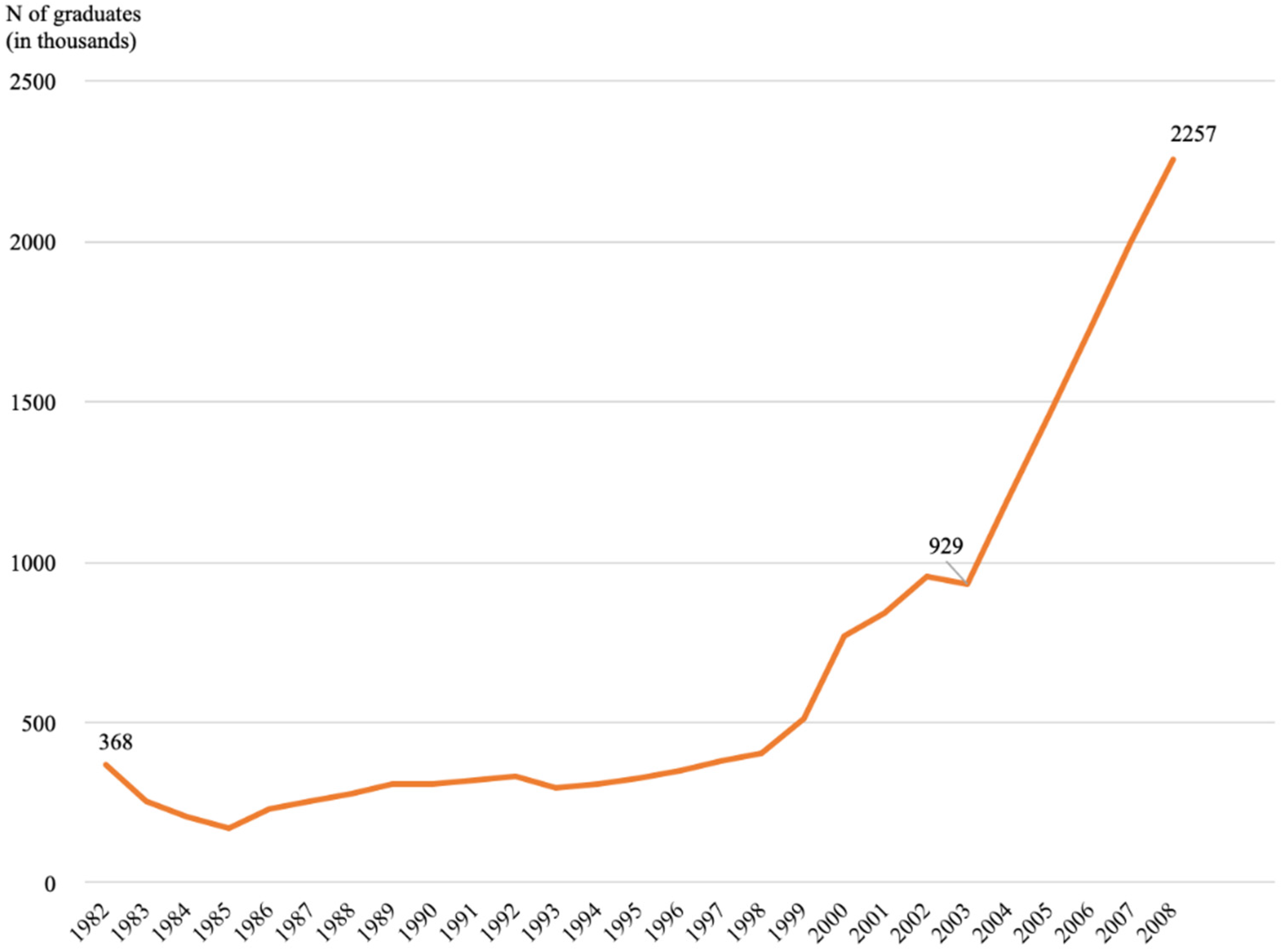
Note that the period under examination corresponds to a substantial surge in the supply of BA-educated labor due to China’s higher education expansion initiated in 1999. Figure 2 shows the number of graduates from 4-year HEIs during 1982–2008, covering all the cohorts of individuals in the sample (i.e., the oldest and youngest men in the sample were scheduled to graduate from 4-year colleges in 1982 and 2008, respectively). Figure 2 indicates that there was a surge in 4-year college graduates starting from 2003. This first after-expansion cohort of 4-year college graduates would enter the labor market starting from 2003, and their earnings would be captured by the paper’s analysis starting from 2004 when they were at least 23 years old. Therefore, the divergent trends for the youngest age groups presented in Figure 1 could be related to the dramatic increases in cohort-specific supply of BA-educated labor, as reflected in Figure 2.
The traditional supply–demand model that assumes perfect substitution across different age groups within the same education level posits that the relative aggregate supply of two types of workers determines their relative wages or wage gap. Under such a hypothesis, we would expect to see parallel trends in wage gaps for workers in different age groups, with their earnings differences fully accounted for by age effects. This framework fails to explain the divergent trends in the BA–HS wage gaps among younger and older workers presented in Figure 1. Therefore, this study extends the basic model to incorporate imperfect substitution among workers of the same education level but in different age groups, and thus allow cohort-specific relative supply of BA-educated labor to directly affect cohort-specific BA–HS wage gaps on top of the effect from shifts of the aggregate relative labor supply curve that equally affects all cohorts.
This study is in the tradition of Card and Lemieux [15], who first proposed a model of labor supply with imperfect substitution between age groups to explain the rising college premium for younger workers and stagnated college premium for older workers during the 1970s–1990s in the US, UK, and Canada. The authors found that the rising college premiums for the baby-boom cohorts are mainly due to a slow-down of the growth in educational attainment for these cohorts, which later translates to a decrease in the cohort-specific relative supply of college-educated labor for these cohorts. These findings suggest that cohorts who encounter substantial changes in the cohort-wide average educational attainment could experience substantial cohort effects due to changes in cohort-specific relative labor supply in addition to the effects equally spread out to all cohorts due to the traditional aggregate relative supply factor. Given the magnitude of China’s higher education expansion, it is interesting to see how the expansion alters the cohort-specific and aggregate relative supply of college-educated labor, and how that in turn affects income inequality between BA- and HS-educated labor in different ages. In the following sections, a theoretical model and empirical analysis are presented to explain the observed pattern in Figure 1 and decompose changes in age-group-specific BA–HS wage gaps into changes in the aggregate and age-group-specific relative supplies of BA-educated labor, and in the aggregate relative demand for BA-educated labor.

4. Theoretical Model

In this section, an aggregate labor supply model is introduced with imperfect substitution across labor with the same education level but in different age groups. For this study, there is a focus on the wage gaps between men whose highest educational levels are either high school or 4-year college (i.e., the BA–HS wage gap). (Three-year junior colleges that grant associate’s degrees (AA) went through substantial institutional reforms and re-structuring during the past decades in China. As a result, the evolution of the AA-HS wage gaps by different age groups over time might be contaminated by changes in the relative quality of 3-year college education and the relative ability of AA-educated labor).
First, the model assumes that there are two types of labor supplied: high school (HS)-educated labor ( L H S ) and 4-year-college (BA)-educated labor ( L B A ), and further assumes that aggregate supply formulas of the two types of labor follow constant elasticity of substitution (CES). Under the traditional aggregate labor supply model that assumes individuals of different ages with the same education level are perfect substitutes for each other, the aggregate supply of HS-educated labor ( L H S , t ) and BA-educated labor ( L B A , t ) at year t can be written as:
L H S , t = j = 1 n α j l H S , j , t
and
L B A , t = j = 1 n β j l B A , j , t
where l H S , j , t and l B A , j , t   are age-group-specific supplies of HS- and BA-educated labor from age group j at year t   , respectively. α j   and β j   are a vector of relative efficiency parameters across age groups for HS- and BA-educated labor, respectively (assumed to be constant across years). Equations (1) and (2) implicitly assume that aggregate supplies of HS- and BA-educated labor are just weighted sums of the quantities of labor supplied by all age groups within the same education levels, respectively. In accordance with Card and Lemieux [15], this assumption is relaxed to allow imperfect substitution across labor with different ages within the same education level. Then, the aggregate supplies of HS-educated labor ( L H S , t ) and BA-educated labor ( L B A , t ) at year t can be written as:
L H S , t = ( j = 1 n α j l H S , j , t   η ) 1 η
and
L B A , t = (   j = 1 n β j l B A , j , t   η ) 1 η
where η = 1 1 σ A , and σ A   is the elasticity of substitution between labor in different age groups j within the same education group. In theory, σ A could be different for BA- and HS-educated labor, and that possibility is dealt with as a robustness check in Section 6.2. In addition, note that under the perfect substitution assumption, σ A = + and η = 1 .
Furthermore, aggregate output at year t   ( y t ) depends on the two sub-aggregates of HS- and BA-educated labor. Aligning with prior literature, this study’s model assumes that the aggregate production function also satisfies constant elasticity of substitution (CES) and thus can be written as follows:
y t   = ( θ H S , t   L H S , t ρ + θ B A , t   L B A , t ρ ) 1 ρ
where ρ = 1 1 σ E , and σ E   is the elasticity of substitution between the two types of labor (i.e., L H S , t and L B A , t ). θ H S , t   and θ B A , t     are the technology efficiency parameters for labor of the two education levels at year t , respectively.
In a competitive labor market and in equilibrium, a HS-educated worker in age group j at year t is paid his/her marginal productivity of labor, and given Equations (3) and (5), we can derive that:
ω H S , j , t = y t l H S , j , t   = y t L H S , t × L H S , t l H S , j , t   = θ H S , t L H S , t ρ η ( θ H S , t L H S , t ρ + θ B A , t   L B A , t ρ ) 1 ρ ρ × α j l H S , j , t   η 1 .  
Similarly, a BA-educated worker in age group j at year t is paid his/her marginal productivity of labor, and given Equations (4) and (5), we obtain the following:
ω B A , j , t = y t l B A , j , t   = y t L B A , t × L B A , t l B A , j , t   = θ B A , t   L B A , t ρ η   ( θ H S , t L H S , t ρ + θ B A , t   L B A , t ρ ) 1 ρ ρ × β j l B A , j , t   η 1 .
Efficient utilization of these two types of labor implies that their relative wages reflect their relative marginal product. Under this condition, the gap between wages measured in natural logarithm of the two types of labor in age group j at year t   can be written as:
r j t ln ( ω j , t B A ω j , t H S ) = ln ( θ B A , t θ H S , t ) + ln ( β j α j ) + ( 1 σ A 1 σ E ) ln ( L B A , t L H S , t ) 1 σ A ln ( l B A , j , t l H S , j , t ) + e j t ,  
where e j t   is the error term that represents sampling variation in the by age group and by year wage gaps. (The error term is assumed to be normally distributed with a mean of zero and a diagonal covariance matrix Σ).
This equation shows that the BA–HS wage gap (or returns to 4-year college or 4-year college premium or BA premium) for the n age groups during the survey years t = 2002, 2003, …, and 2009, are affected by the following factors: “ ln ( θ B A , t θ H S , t ) ” is the relative technology efficiency parameters of the two types of labor at year t , which affects the relative demand for the two types of labor; “ ln ( β j α j ) ” is the relative efficiency parameters across age groups, which leads to age effects among workers of different ages; “ ( 1 σ A 1 σ E ) ln ( L B A , t L H S , t ) ” is the aggregate relative supply of BA- vs. HS-educated labor at year t ; and “ 1 σ A ln ( l B A , j , t l H S , j , t ) ” is the age-group-specific relative supply of the two types of labor for age-group j at year t . Equation (8) shows that the BA–HS wage gaps depend on both the aggregate supply of BA- and HS-educated labor in the labor market (i.e.,   L B A , t L H S , t ), and the corresponding age-group-specific supply of respective labor within his own cohorts (i.e., l B A , j , t l H S , j , t ).
Following the previous literature, that often assumes that there is a log-linear increasing trend in the demand for skills over time caused by skill-biased technological change [8,31,32], the relative technology parameter between the two types of labor at year t, which is the first term in the right hand-side of Equation (8), can be further simplified as:
ln ( θ B A , t θ H S , t )   =   λ 0 λ 1 t
where t is survey year or time period 1, 2, …, 8 for this case, and the coefficient on this time trend term (i.e., λ 1) represents the annual growth rate in the relative demand for BA-educate labor. In addition, note that the second term in the right hand-side of Equation (8) [i.e., ln ( β j α j ) ] represents relative efficiency between BA- and HS-educated labor for age group j and can be captured using a series of age dummies (i.e., A g e j ). Therefore, Equation (8) can be further re-written as:
r j t = λ 1 t + λ j A g e j + λ 3 ln ( L B A , t L H S , t ) + λ 4 ln ( l B A , j , t l H S , j , t ) + λ 0 + e j t
that is, we can decompose the BA–HS wage gap (or the BA premium) for age group j in year t into a linear time trend that accounts for skill-biased technological changes, and age effects for the n age groups, as well as aggregate and age-group-specific relative labor supply factors.

5. Data, Sample and Key Variables

This section presents an empirical analysis that identifies all the parameters in Equation (8). The main focus is on the estimates before the age-group-specific [i.e., 1 σ A in Equation (8) or λ 4   in Equation (10)] and aggregate [i.e., ( 1 σ A 1 σ E ) in Equation (8) or λ 3   in Equation (10)] relative labor supply terms: the former could help explain the fall in college premiums particularly accrued to younger cohorts, and the latter could capture any spill-over effects from a surge in the supply of young college-educated labor on older cohorts in the labor market (i.e., who were not directly “treated” by the higher education expansion). The following paragraphs elaborate on the data and sample used, how key variables were constructed, and the estimation procedures to identify model parameters.

5.1. Data

This study’s major source of data is the Urban Household Survey (UHS), conducted annually by China’s National Bureau of Statistics (NBS). The UHS is the only nationally representative microdata that covers all provinces in China and has been conducted in consecutive years since the late 1980s [56,57] (There are some major changes in sampling methods and survey questionnaires in 2002 [57], and very few have access to data after 2009. To the author’s knowledge, only one study [56] uses data from UHS 2010–2012, that only covers four provinces in China. Recent studies [58,59,60] that use the UHS to study topics such as employment, earnings and consumption, predominantly use data from the 2002–2009 survey rounds). The UHS adopts a probabilistic and stratified multi-stage sampling method to obtain samples that are representative of urban China for each round [51]. (The UHS samples one third of the same households from the previous year and replaces all the households every three years. Sampling method and the assigning of sampling weights are consistent at least for the 2002–2009 rounds of the UHS dataset [56,57]). This paper accessed a random subset of the UHS full sample for the years between 2002–2009. The subset for these eight rounds covers 9 provinces that are representative of the total 31 provincial districts in mainland China. (The nine provinces are: Beijing, Shanxi, Liaoning, Jiangsu, Anhui, Guangdong, Chongqing, Sichuan, and Gansu. The 2003 round of the UHS has 7 additional provinces; however, to keep it consistent across survey years, the author dropped individuals from these additional provinces for the UHS 2003 round). This time has the advantage of capturing the labor market dynamics when there are presumably substantial increases in both the supply and demand of college-educated labor. On top of this survey data, this paper also uses statistics from the Educational Statistics Yearbook of China and the NBS’s national data archive [55] to construct macro-level measures of various supply variables.

5.2. Sample

The analysis sample is restricted to men born during 1960–1986, corresponding to the 1978–2004 probable college cohorts (majority students in China finish high school and attend college at age 18; men in the sample are scheduled to attend college in 1978–2004). People older than these cohorts were affected by the Cultural Revolution, during which most educational institutions were disrupted and the college entrance exam (i.e., a prerequisite for attending college) was cancelled; people younger than these cohorts might not have completed 4-year college and worked for at least an entire year by 2009. The sample is later divided into five age groups according to an individual’s age at time of the survey (explained in more details in the next sub-section); and to ensure that the age ranges are consistent across survey years, the sample only keeps men aged 23 to 42 years old at the time of the survey. (There are two additional reasons for focusing on men aged between 23 and 42: first, these cohorts are comparable in terms of their access to HEIs, and second, people older than this age range are more likely to pursue higher education after some years of work, mostly for job promotion purposes, making the age-group-specific supply variable (constructed under the assumption that people work right after completing their highest level of education as will be explained later in Section 5.3) inaccurate for older age groups). Similar to many previous studies referenced above, this paper first focuses on male workers to avoid cofounding influences from any inter-cohort or temporal changes in female labor supply. (The papers later present results from use of the sample that includes both females and males as a robustness check in Section 6.) This paper is further restricted to individuals whose highest educational attainment was either high school (including academic and vocational high school) or 4-year college and drops those with other levels of educational attainment (e.g., those who never attended high school, attended 3-year junior colleges, or graduate schools). Finally, the paper excludes those who were enrolled in school, had a long-term illness, or retired at the time of the survey. The full analysis sample pooled across eight survey rounds contains 52,483 male individuals, and the sample size for each survey round ranges from 5216 to 9916.

5.3. Key Variables

5.3.1. Indicators for Age Groups

Five indicator variables were created to indicate whether an individual is in the age ranges of [23, 26], [27, 30], [31, 34], [35, 38] or [39, 42] at the time of the survey. The construction of the age groups ensures that the youngest cohort surveyed at the latest round (i.e., 2009) and the oldest cohort surveyed at the earliest round (i.e., 2002) can cover all the cohorts for the analysis sample (i.e., the 1960–1986 birth cohorts, or the 1978–2004 probable college cohorts). Moreover, by starting from individuals aged 23 years old, this can ensure that graduates from 4-year colleges have worked for at least an entire year at the time of the survey. Age-group-specific measures of wage gaps and labor supplies for these five age groups, respectively, were then constructed.

5.3.2. BA–HS Wage Gap

The “educational attainment” variable in the UHS asks individuals to report their highest level of schooling attended, no matter if the individual completed it and obtained a degree or not. Two dummy variables were created, “BA” and “HS”, to indicate whether an individual had ever attended a regular 4-year college and high school as their highest “educational attainment”, respectively.
As for earnings, the UHS records four sources of annual income: labor, business, assets, and transfers. Annual labor income was used and all the income variables were inflated to the 2020 Chinese currency value using annual nationwide CPIs in urban areas [55]. Labor income (wages and salaries) can better reflect equilibrium wages paid for the two types of labor in the labor market, and in practice, other categories of income have a higher proportion of missing values. Results are approximately identical if instead total income is used, that adds up all four sources of income; but the sample size severely shrinks when using total income instead of labor income.
To compute the age-group-specific BA–HS wage gaps for each survey year (i.e., r j t ) , first, compute the mean log annual employment income within each age group–survey year cell separately for BA- and HS-educated men. Then, the wage gap is derived as the difference in log mean income between the BA and HS groups within each age–year cell. By using log earnings, this restricts the analysis to those who earn non-zero employment income at the time of the survey (approximately 90% of the full analysis sample earn positive employment income at the time of the survey). Table 2 below lists the by year and by age group BA–HS wage gaps in logarithmic form.

5.3.3. Age-Group-Specific Supply of BA- and HS-Educated Labor

Ideally, the best way to construct the age-group-specific relative labor supply measure is to use the quantity of efficient labor supplied by workers within each educational level and age group for each year. For example, Card and Lemieux [15] use CPS data on the sums of actual hours supplied by all workers within each age-education-year cell to construct this measure. However, information on an individual’s yearly hours worked is unavailable for the UHS dataset. Instead, the total number of high school and 4-year college graduates in each age group-year cell was used to estimate the potential quantity of age-group-specific supply of HS- and BA-educated labor, respectively. (The labor force participation rate for male workers is constantly high in China: it ranges between 79–82 percent during 2002–2009 [61]). More specifically, the paper assumes that students graduate from high school and 4-year college at 18 and 22 years old, respectively, and assumes that individuals would directly enter the labor market when they graduate, if not pursuing further studies. Therefore, as an example, age-group-specific supply of BA-educated labor within the 23–26 age group at year 2009 ( l B A ,   2326 , 2009 ) would be the sum of graduates from 4-year colleges minus the sum of students who continue to attend graduate schools, at the master’s level (there are very few college graduates who are directly admitted into doctoral programs; therefore, here, the paper uses the number of new admits into master’s programs instead of into any graduate programs (master’s and doctoral programs combined)) during the years of 2005–2008 (i.e., the 23–26-year-olds BA-educated labor in 2009 should have graduated from 4-year college in 2005–2008). Similarly, age-group-specific supply of HS-educated labor within the 39–42 age group at year 2002 ( l H S , 3942 , 2002 ) would be the sum of graduates from high school minus the sum of students who continue to attend 3- or 4-year colleges during 1978–1981 (i.e., the 39–42-year-old HS-educated labor in 2002 should have graduated from high school in 1978–1981). The number of graduates is used, instead of the number of degrees conferred, to better correspond to the “educational attainment” measure used in the UHS. The paper also adjusts for gender differentials in labor force participation and working hours when summing up male and female graduates for a given year by using female labor supply weight for that year. Data on the number of high school and 4-year college graduates, as well as number of new enrollments into 3-year colleges, 4-year colleges, and graduate schools (at the master’s level) for each year during the years between 1978 and 2008 come from the Educational Statistics Yearbook of China. (The Educational Statistics Yearbook of China reports total number of students and the number of female students in each educational level in each year). Given the age-group-specific quantities for the two types of labor, the age-group-specific relative labor supply variable ( l B A , j , t l H S , j , t ) is computed as the ratio between BA- and HS-educated labor within each age group-survey year cell.
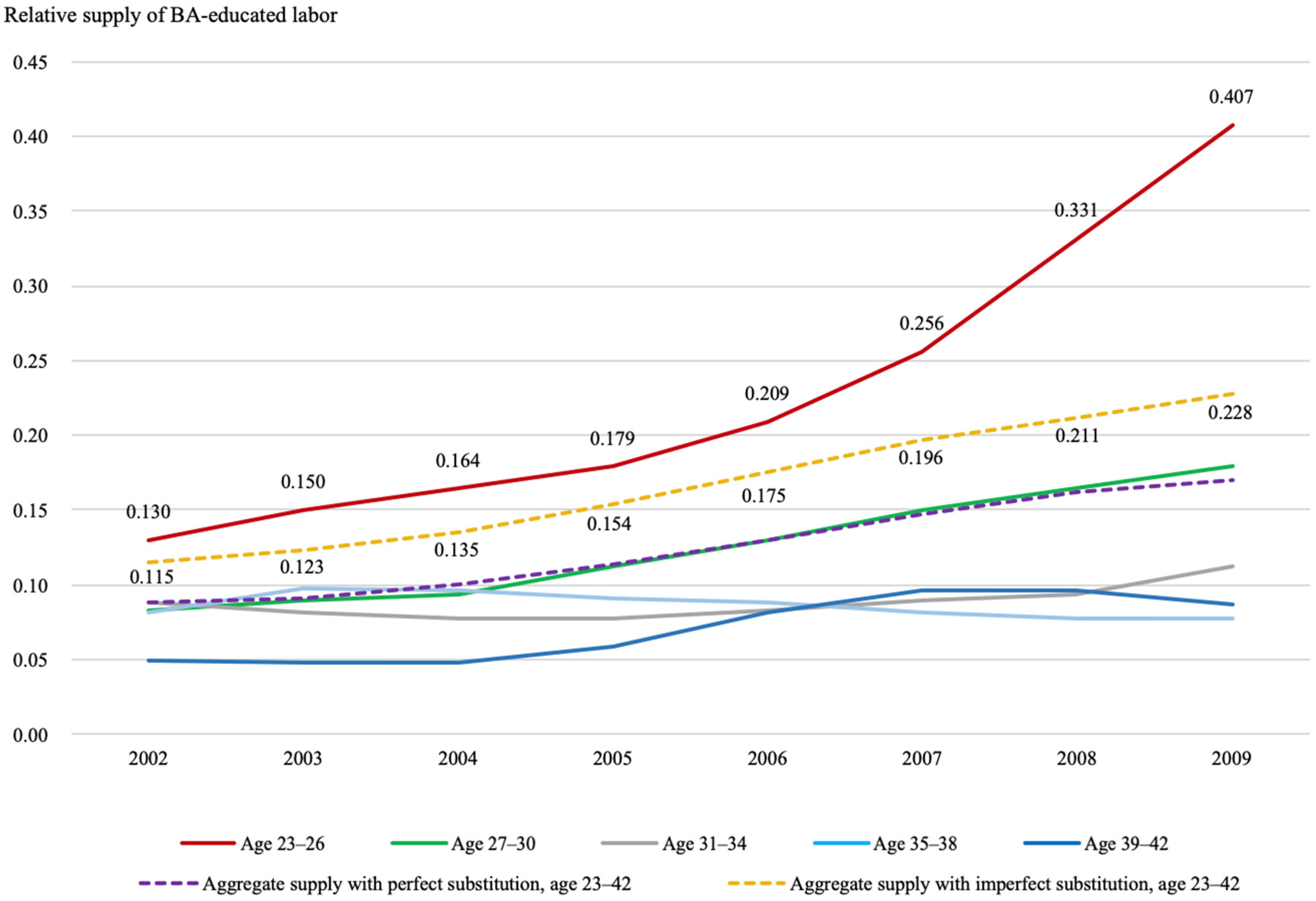
The top panel in Table 3 below presents the constructed age-group-specific relative supply index by year, and Figure 3 shows it graphically. For all the age groups except for the 35–38 group, the ratio of BA-educated vs. HS-educated labor increases from 2002 to 2009. However, the increases are much steeper for the youngest groups: for 23–26-year-olds in 2002, the ratio is 13%, and it more than triples (i.e., increases by approximately 213%) to reach 41% by 2009; for the 27–30 age group, this ratio increases by about 116% from 2002 to 2009.

5.3.4. Aggregate Supply of BA- and HS-Educated Labor

For this study, aggregate supplies are measured using male workers in the [23, 42] age range, and to make comparisons, the aggregate labor supply measures are constructed under the hypotheses of both perfect and imperfect substitution across age groups.
1. Aggregate labor supply with perfect substitution across age groups; Given perfect substitution across age groups [(i.e., see Equations (1) and (2)] and assuming that labor in different age groups supply the same efficiency unit of labor, the sub-aggregates of HS-educated labor ( L H S , t ) and BA-educated labor ( L B A , t ) at year t can be written as:
L H S , t = j = 1 n l H S , j , t
and
L B A , t = j = 1 n l B A , j , t
That is, given age-group-specific labor supplies for the five age groups at each survey year t , the aggregate supply of BA- and HS-educated labor are a simple sum of the five age groups within each survey year. Given the aggregate quantities of BA- and HS-educated labor supplied in each year, the aggregate relative supply term in Equation (8) (i.e., L B A , t L H S , t ) is computed as the ratio between the aggregate supplies of two types of labor at year t .
2. Aggregate labor supply with imperfect substitution across age groups. According to Equations (3) and (4), given age-group-specific supplies for the two types of labor at each year, we still need to know the elasticity of substitution across age groups (i.e., σ A ) and the relative efficiency parameters across age groups for the two types of labor (i.e., α j   a n d   β j ) to compute aggregate supply of BA- and HS-educated labor under imperfect substitution across ages. This sub-section briefly introduces the method to first derive σ A ,   α j , a n d   β j , and then construct the aggregate labor supply measures.
Note that according to Equation (8), the BA–HS wage gaps for age group j at year t are affected by a set of year effects that are fixed across age groups [i.e., “ ln ( θ B A , t θ H S , t ) ” and “ ( 1 σ A 1 σ E ) ln ( L B A , t L H S , t ) ”], a set of age-group-specific factors that are constant across years [i.e., “ ln ( β j α j ) ”], and a set of age-group-specific factors [i.e., “ 1 σ A ln ( l B A , j , t l H S , j , t ) ”]. This implies that Equation (8) can be re-written as:
r j t = δ t Y e a r t + γ j A g e j 1 σ A ln ( l B A , j , t l H S , j , t ) + e j t ,
that is, the BA–HS wage gaps can be decomposed into survey year effects (i.e., Y e a r t ), age effects, an additional age-group-specific (or “cohort”) effect, and coefficients on these terms ( δ t , γ j , and 1 σ A ) estimate the magnitudes of these effects accordingly. Under perfect substitution across age groups, there will be no additional cohort effects after controlling for year and age effects (i.e., 1 σ A   = 0). We can use Equation (13) to empirically estimate 1 σ A by regressing age-group-survey-year level BA–HS wage gaps on the eight survey year dummies, the five age-group dummies, and age-group-survey-year level relative supplies of BA- vs. HS-educated labor. The coefficient on the “age-group-specific relative labor supply” term ( ln ( l B A , j , t l H S , j , t ) ) would give an estimate of 1 σ A . Using the analysis sample of this study, the estimate of 1 σ A is approximately 0.2 (i.e., σ A = 5), which is in line with the estimates derived using data from the US, UK, and Canada (i.e., σ A   is estimated to be in the range of 4–6 for the three countries) [15].
Given the estimate of σ A , the second step is to identify the relative efficiency parameters across age groups for the two types of labor α j   a n d   β j . Note that if we take logs of both sides of Equation (6), we can obtain:
ln ( ω H S , j , t ) = ln φ + ln ( α j ) 1 σ A ln ( l H S , j , t )
where φ = θ H S , t   L H S , t ρ η   ( θ H S , t   L H S , t ρ + θ B A , t   L B A , t ρ ) 1 ρ ρ captures all the survey year effects. It could be further simplified as:
ln ( ω H S , j , t ) + 1 σ A ln ( l H S , j , t ) = ϵ H S , t Y e a r t + ln ( α j )
Similarly, re-writing Equation (7), we can obtain:
ln ( ω B A , j , t ) + 1 σ A ln ( l B A , j , t ) = ϵ B A , t Y e a r t + ln ( β j )
The left-hand side of Equations (15) and (16) are easily computed using mean log wages and age-group-specific labor supplies within each education-age-year cell, as well as the 1 σ A estimated from the first step. Then, we can run regressions of the left-hand side sums on the survey year dummies and age group dummies for HS- and BA-educated labor, respectively. Coefficients on the age group dummies in Equations (15) and (16) would give us the estimates of α j   and β j , respectively.
Given estimates of σ A , α j   and β j , we can compute the aggregate supply of the two types of labor at a given year t ( L H S , t   and L B A , t ) using Equations (3) and (4), and the aggregate relative labor supply variable ( L B A , t L H S , t ) accordingly. The bottom panel in Table 3 presents the aggregate relative labor supply measures under perfect and imperfect substitution across age groups, and the dotted lines in Figure 3 plots them graphically. In general, the trends in aggregate relative labor supply during 2002–2009 are similar under the two hypotheses. However, the measures under imperfect substitution across age groups are higher than those under perfect substitution, and the increases in these measures over time are larger under the “imperfect substitution” hypothesis.

6. Results

6.1. Basic Model

Using variables constructed in Section 5, we can use Equation (10) to decompose the BA–HS wage gap (or the BA premium) for age group j in year t into age-group-specific and aggregate relative labor supply factors, a linear time trend that accounts for skill-biased technological changes, and age effects. Table 4 below presents results from the decomposition using ordinary least squares (OLS) regressions. Model 1 first presents regression results from using Equation (13) that decomposes the BA–HS wage gaps into an age-group-specific relative labor supply factor, year effects, and age effects. Models 2 and 3 replace survey year fixed effects with a linear “time trend” term using Equation (10). Model 2 uses the aggregate relative labor supply measure constructed under perfect substitution across age groups hypothesis, and model 3 adopts the measure created under imperfect substitution across age groups hypothesis.
There are several key findings in Table 4. First, coefficients on the “age-group-specific relative labor supply” measure are all statistically significantly different from 0 for the three models, and the magnitudes of the coefficients are quite similar across different model specifications. Note that the coefficient estimated using model 1 (i.e., -0.199) would give an estimate of 1 σ A , and result shows that labor in different age groups within the same education group is strong but not perfect substitutes. This also implies that there are substantial cohort effects on BA–HS wage gaps after controlling for the effects due to shifts in aggregate relative labor supply and demand curves that affect all cohorts.
Second, comparing across the three models, the R-square is highest for model 3, suggesting that a model of aggregate relative labor supply with imperfect substitution across age groups fits the empirical data the best. Moreover, the paper will show later that the coefficients on the “aggregate relative labor supply” and “annual temporal trend” variables are much easier to interpret in model 3 under imperfect substitution than in model 2 under perfect substitution.
Third, the “age effects” estimated under the three models are also quite similar: holding other conditions constant, the college premium is the lowest for the youngest age group in the sample, increases substantially for workers between 27 and 38 years old, and the premium drops as people grow even older (but is still statistically significantly higher than the youngest age group).
Lastly, the paper focuses on interpreting the coefficients in model 3. The primary interest is the coefficient on the “age-group-specific relative labor supply” variable that is estimated to be approximately −0.2. The magnitude of the coefficient means that when the supply of BA-educated labor (relative to HS-educated labor) increases by 1% within one’s own age group, there will be an additional 0.2% decrease in the BA–HS wage gap particularly for this age group, on top of the effects that affect all age groups. For example, the relative labor supply measure for the youngest age group (i.e., 23–26 years old) jumps from 0.13 in 2002 to 0.41 in 2009, a 213% increase. Consequently, the coefficient on the cohort effects implies that the BA–HS wage gap for men aged 23–26 is estimated to be about 42.6% lower in 2009 as compared with that for men of the same ages in 2002, due to the cohort-specific relative labor supply factor.
Apart from the age-group-specific labor supply factor that accrued to particular cohorts, the “annual temporal trend” and “aggregate relative labor supply” terms capture changes in aggregate relative demand and supply of BA-educated labor over time that affect workers in all age groups in the labor market. More specifically, coefficient on the “temporal trend” term (or the annual growth rate of the relative technology parameter) is estimated to be 0.095. This means that BA–HS wage gaps increased by about 9.5% annually for all age groups during 2002 to 2009, due to skill-biased technology change that raised the demand for BA-educated labor (relative to HS-educated labor). The estimates of the effects of technological progress on BA–HS wage gaps are higher than previous work for developed countries during 1960s and 1990s [8,15,32]. Note that the sampled time witnesses an increasing degree of trade openness and large inflow of foreign direct investment (FDI), as well as rapid growth of GDP (the average annual GDP growth rate is 10.8% between 2002 and 2009). Meanwhile, the temporal trend in favor of BA-educated labor is mitigated by increases in the aggregate relative supply of BA-educated labor: the coefficient on the aggregate relative labor supply measure in model 3 (i.e., −0.56) is statistically significant and negative. Note that the aggregate relative labor supply measure grows by about 98% from 2002 to 2009 (i.e., from 0.115 in 2002 to 0.228 in 2009), suggesting that the BA premium is predicted to drop by 55% from 2002 to 2009 due to this aggregate relative labor supply factor. Combined, the coefficients on the aggregate relative labor demand and supply indexes predict that the BA–HS wage gaps rise at an annual rate of around 1.7% for all age groups in the sample. This aligns with the growth trajectory of the sample mean BA–HS wage gaps illustrated in Figure 1. These effects due to shifts in the aggregate labor supply and demand curves are equally spread out to men of all ages, on top of the “cohort effects” for particular age groups mentioned in the previous paragraph.
Combining the cohort effect with effects for all age groups, we can see that the BA–HS wage gap for men of 23–26 years old is predicted to be approximately 31% lower (1.7 × 7 – 42.6) in 2009 than that for men of the same age range in 2002. For the age groups that do not experience fast growth in age-group-specific relative supply of BA-educated labor, BA–HS wage gaps would be larger in 2009 than in 2002. For example, using the relative labor supply measure for the 35–38 age group presented in Table 3, the BA–HS wage gap for men aged 35–38 years old is predicted to be about 13% larger in 2009 than that for men of the same ages in 2002.

6.2. Robustness Checks

This paper evaluated the robustness of results found in Table 4 to other sample selections and alternative specifications. First, the focus so far has been on the BA–HS wage gaps for male workers only, partly for fear of any composition effects due to changes in female labor supply both across cohorts and over time. Below, a robustness check is conducted to see whether results presented in Table 4 are robust to the inclusion of female workers. Table 5 below reports same sets of results using both female and male workers to compute the BA–HS wage gaps.
Using the sample that pools males and females together, estimates on the “age-group-specific relative supply” variable across the three models are still statistically significantly different from 0, and range from −0.18 to −0.16, which are quite close to the parameters estimated using the “males only” sample (i.e., −0.20 to −0.19). When comparing model 3 in Table 4 and Table 5, the negative effect of age-group-specific relative supply becomes slightly smaller when including female workers (i.e., 0.163 in Table 5 vs. 0.195 in Table 4), while the negative effect of aggregate relative supply under imperfect substitution hypothesis becomes larger (i.e., 0.833 in Table 5 vs. 0.560 in Table 4). The estimate on the annual “time trend” variable shrinks by about 16% when including female workers (i.e., 0.079 in Table 5 vs. 0.095 in Table 4). The major take-away from comparing Table 4 and Table 5 is that the general pattern of results and estimated parameters on key variables (e.g., the cohort effect term) in Table 4 are quite robust to different sample selections. Note that though the sample size becomes larger when including female workers, the R-squares when using a combined sample of females and males are uniformly lower than the corresponding R-squares when using the males-only sample, which implies that there are larger proportion of unexplained variation in wage gaps apart from labor supply and demand factors for female workers than for male workers. For this reason and for the sake of brevity, there is a focus on the male workers sample for the main analysis throughout this study.
Second, the proposed model in Section 4 assumes that the elasticity of substitution between labor in different age groups j within the same education group (i.e., σ A ) is the same for BA- and HS-educated labor. We can relax this assumption and allow different substitution elasticities for the two types of labor. Under the latter case, Equation (14) would be written as:
ln ( ω H S , j , t ) = ln φ H S + ln ( α j ) 1 σ A H S ln ( l H S , j , t )
where σ A H S is the elasticity of substitution between HS-educated labor in different age groups j, and all others are defined the same way as in Section 4 (i.e., φ H S = θ H S , t   L H S , t ρ η   ( θ H S , t   L H S , t ρ + θ B A , t   L B A , t ρ ) 1 ρ ρ captures all the survey year effects). Similarly, with BA-educated labor:
ln ( ω B A , j , t ) = ln φ B A + ln ( β j ) 1 σ A B A ln ( l B A , j , t )
where σ A B A is the elasticity of substitution between BA-educated labor in different age groups j, and φ B A = θ B A , t   L B A , t ρ η   ( θ H S , t L H S , t ρ + θ B A , t   L B A , t ρ ) 1 ρ ρ captures all the survey year effects. Using the same method as presented in Section 4 (i.e., regress log wages on age-group-specific supplies separately for the HS and BA groups, both with age group and survey year dummies), the coefficients on the age-group-specific labor supply terms for the HS- and BA-educated labor would give estimates of σ A H S   and   σ A B A , respectively. Results show that age-group-specific supplies have negative and statistically significant effects on both HS and BA wages, and the estimates of 1 σ A H S   and   1 σ A B S are approximately 0.17 and 0.14, respectively, suggesting that the negative cohort effect seems to be larger for HS-educated labor (or HS-educated labor has a lower degree of substitution across age groups than BA-educated labor). Card and Lemieux [15] also find that highly educated labor has a higher degree of substitution among workers in different age groups. The magnitudes of these elasticities are also fairly close to the one estimated using the basic model presented in Section 4 (i.e., 1 σ A H S = 1 σ A B S = 0.2 ).
Lastly, the results are tested to determine if they are robust to the definition of HS- and BA-educated labor. As mentioned in Section 5.3.3, this paper defines labor supply measures of HS- and BA-educated labor using the number of graduates from the respective educational levels, regardless of whether the individual obtains the corresponding degree or not. As an alternative, those who actually obtain the degrees are distinguished from those who do not by assigning weights equal to their relative wage within both the BA and HS groups: for example, high school dropouts are weighted by their relative average wage to high school graduates with a diploma; those who attend 4-year college without obtaining a degree are weighted by their relative average wage to college graduates who obtained a bachelor’s degree (As mentioned before, the UHS 2002–2009 dataset defines its only “education attainment” variable as the highest educational level attended. To calculate the weights, data from a comparable dataset is used—the Chinese Household Income Project (CHIP) that draw its samples from the larger UHS sample [62], and has more detailed questions regarding educational attainment. CHIP has two rounds during 2002–2009, and weights calculated using either the CHIP 2002 or CHIP 2008 wave are nearly identical). All the models in Table 4 are then re-run using these alternative labor supply measures. The pattern of results barely changes, and the magnitude of the estimate on the age-group-specific supply measure marginally changes to be smaller. For the sake of brevity, the estimates of the new supply measures and regression results are not presented in the text, but they are available upon request from the author.

7. Relative Supplies and Predicted Wage Gaps after 2009

Section 4, Section 5 and Section 6 build a model of relative wage determination that allows for the relative wage to endogenously adjust to shifts in the supply and demand of different types of labor over time and use annual data from 2002–2009 to specify all the model parameters. This paper has shown that the model well explains the evolution of the BA–HS wage gaps in the labor market during 2002–2009. In addition, one strength of such a structural model is that it can predict out-of-sample scenarios and simulate policy counterfactuals beyond the specific context and samples from where the parameters are derived from [63]. In this section, the model and estimates of the relative supply measures beyond 2009 are used to predict wage gaps after 2009. One could also use the model to simulate other policy scenarios (e.g., if there were no radical increases in college graduates since 2003, what trajectories the relative supply measures would follow and what the corresponding wage gaps under such circumstances would be). In this section, estimates of the age-group-specific and aggregate relative supply of BA-educated labor after 2009 are presented and corresponding wage gaps are predicted using parameters identified in model 3 of Table 4. To probe how well this proposed model could predict out-of-sample scenarios, the predicted wage gaps in 2013 and 2018 are cross-checked with the actual wage gaps estimated using the 2013 and 2018 waves of data from the Chinese Household Income Project.

7.1. Relative Supplies of BA-Educated Labor after 2009

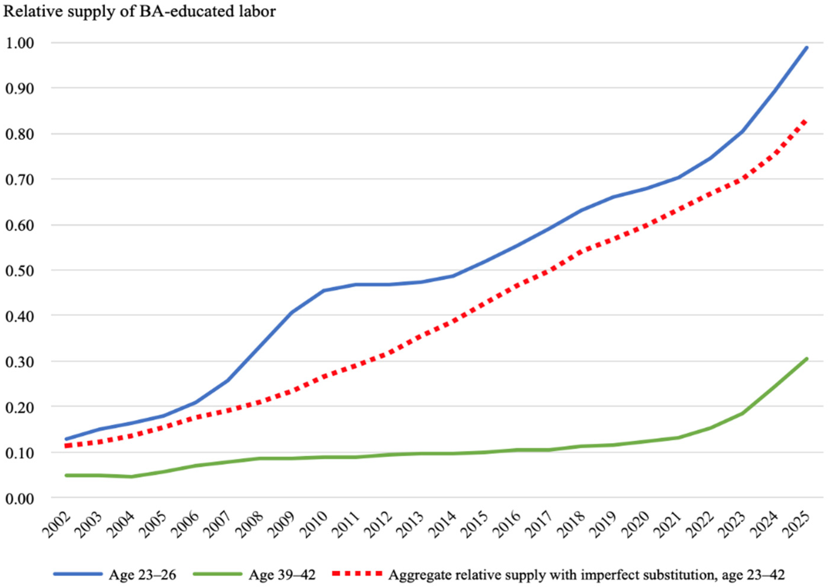
Table 6 below presents estimates of age-group-specific relative supply of BA-educated labor during 2010–2025. For the years between 2010–2021, the actual number of graduates and newly admitted students is used and the relative supply measures are calculated using the same method introduced in Section 5.3.3. For BA-educated labor in the 23–26 age group for years 2022–2025, the projected number of BA graduates in 2022–2025 is used, that are predicted using the number of newly enrolled students in 4-year colleges in 2018–2021, adjusted by a graduation probability for each year. The number of new enrollments in master’s programs in 2022–2025 is predicted based on the actual number of new enrollments for the previous years, assuming new enrollments follow a linear time trend. The last row in Table 6 shows estimates of the aggregate relative supply measure with imperfect substitution among age groups using the same method explained in Section 5.3.4. Figure 4 presents the aggregate relative supply measure and age-group-specific measures for the youngest and oldest age groups from 2002 to 2025.
Table 6 indicates that age-group-specific relative supplies of BA-educated labor rise for all age groups during 2010–2021 and are predicted to keep increasing afterwards. Figure 4 shows that for the youngest age group in the sample (the “23–26” age group), the age-group-specific relative supply rose during 2002 and 2011, with sharp increases during 2005 and 2009; the relative supply stayed constant between 2011 and 2014, and then gradually increased since 2015. For the “39–42” age group, the age-group-specific relative supply of BA-educated labor stayed relatively stable until 2019; starting from 2020, relative supply of BA-educated labor for the “39–42” age group began to increase and underwent large jumps from 2022 onwards. Note that the oldest cohort in the “39–42” age group at year 2020 were scheduled to attend college in 1999 (i.e., the first year of the college expansion program), and the “39–42” age group after 2020 would start to pick up more and more cohorts of BA-educated labor who attended college after the expansion. Combined, Figure 4 suggests that the effect of college expansion on the age-group-specific relative supply of BA-educated labor appears most influential for younger age groups during the first decade of the 21st century; while, when the post-expansion cohorts of BA-educated labor grow older, the college expansion starts to affect older age groups in recent years. Meanwhile, the aggregate relative supply of BA-educated labor keeps increasing from 2002 to 2025, which would affect the BA–HS wage gaps for all age groups.

7.2. Predicted BA–HS Wage Gaps after 2009

Given estimates of the age-group and aggregate relative supply of BA-educated labor during 2010 and 2025 that are shown in Table 6, we can use parameters presented in model 3 of Table 4 to calculate age-group-specific wage gaps for the years between 2010 and 2025, under the assumption that parameters specified using empirical data for the years of 2002–2009 keep constant for years after 2009. More recent rounds of data from the UHS are unavailable to test this assumption; however, two recent rounds of data from a comparable dataset are used to estimate age-group-specific wage gaps in 2013 and 2018 and compare them to the predicted wage gaps from the identified model. (More specifically, the 2013 and 2018 waves of the Chinese Household Income Project (CHIP) are used, which draws its samples from the larger UHS sample [62] and administers similar questions regarding respondents’ employment status, earnings, and education attainment, etc.). Table 7 below presents results from the prediction and comparison for selected years.
The column under year 2009 in Table 7 repeats age-specific and sample mean wage gaps in 2009 that are listed in Table 2. Wage gaps in 2009 are used as the baseline level, and the first column under each year presents predicted changes in wage gaps for that year from their corresponding baseline level in 2009. Take the wage gap for the “23–26” age group in 2013 as an example: its age-group-specific relative supply increases by 16% from 2009 to 2013 (i.e., from 0.407 in 2009 to 0.473 in 2013), and meanwhile the aggregate relative supply of BA-educated labor increases by 55% (i.e., from 0.228 in 2009 to 0.354 in 2013), then the estimated change in the wage gap specifically for this age group from 2009 to 2013 would be approximately 4% (i.e., 0.195 × 0.16 0.560 × 0.55 + 0.095 × 4 = 0.041 ). The second column under each year presents the corresponding predicted age-group-specific and sample-mean wage gaps for each selected year. The third column under years 2013 and 2018 lists the actual wage gaps in 2013 and 2018 respectively estimated using the CHIP datasets.
There are several key take-aways from Table 7. First, for the five years presented, the sample mean BA–HS wage gaps go all the way down from 2009 to 2015. It is predicted to be approximately 35% in 2022, a 38% decrease from the 2009 level, and is predicted to decrease further to be about 20% in 2025 (a 65% drop from the 2009 level). Second, for age-group-specific wage gaps, there is a different pattern for younger and older workers: wage gaps have been trending downwards for younger age groups (except for a couple of outstanding years), but for the older age groups, their age-group-specific wage gaps have been kept quite unchanged until recently. For example, the wage gap increases a little bit in 2013, and experiences slight drops in 2018 and 2022 for the 39–42 age group. Whereas the wage gap for this oldest age group is predicted to drop by 58% in 2025. As has been pointed out before, by 2025 the “39–42” age group has picked up cohorts who attended college after the expansion. In other words, the college expansion seems to mostly depress wage gaps for younger age groups during earlier years but would substantially narrow down wage gaps for all age groups starting from recent years and in the near future. Moreover, note that the “23–26” age group in 2009 corresponds to the 1983–1986 birth cohorts who would be scheduled to attend college in 2001–2004 (i.e., the first years after the college expansion). These cohorts would be captured by the “27–30” age group in 2013 and the “39–42” age group in 2025. Results in Table 7 imply that these birth cohorts have lower BA–HS wage gaps compared with those for preceding cohorts when both are in their twenties and early forties, respectively. If longer period of longitudinal or panel data are available, it is interesting to follow these certain cohorts to see how radical expansion of college attendance affects their lifelong earnings. Finally, comparing model 2 and model 3 for the years 2013 and 2018 shows that predicted values of both age-group-specific and sample-mean wage gaps are reasonably close to those estimated using the CHIP datasets, which provides confidence in the credibility for the identified model and its power of predicting out-of-sample scenarios.

8. Discussion and Conclusions

This study builds a model of aggregate labor supplies with imperfect substitution across labor with the same level of education but in different ages to depicts changes in the age-specific BA–HS wage differentials in recent decades in urban China and decomposes the changes into age-specific and aggregate relative labor supply and demand factors. Given the scale of China’s college expansion and thus large variation in the average level of college attainment across cohorts, the traditional methods used to estimate the relative supply of college-educated labor (i.e., aggregates of labor with the same education across all ages, assuming perfect substitution) and the Mincerian returns to college (i.e., weighted average returns across all ages) mask important cohort variation in both relative labor supplies and wage gaps. On the other hand, modern approaches that use experimental and quasi-experimental methods (for example, randomized controlled trials, instrumental variable, regression discontinuity, difference-in-differences, etc.) to estimate the causal relation between education and earnings may not apply very well in this context because these methods assume that skill prices in the labor market are fixed as an individual is “treated” (usually when he/she gets more education). These methods are most effective in micro-interventions when the assumption of “no spill-over effects to untreated individuals” works best, but this assumption may not hold during China’s college expansion (i.e., individuals who attended college before the expansion would also be affected by any changes in the equilibrium price for skill in the labor market as more and more post-expansion college-educated labor enter the labor market). Methodologically, this model of aggregate supplies with imperfect substitution across labor of the same education but in different age groups allows for age-group-specific relative supplies of college-educated labor to affect both age-group-specific and the overall college premiums, and therefore empirically tests the magnitudes of both cohort effect and spill-over effect of the expansion. Results from this analysis can thus reveal the general equilibrium effects of college expansion on urban China’s wage structure (at both the cohort and aggregate levels) in recent decades and predict what these impacts are likely to be in the future.
Results from this analysis show that the sample mean BA–HS wage gaps have been risen modestly during 2002–2009. Meanwhile, workers aged 23–30 years old experience decreasing wage gaps, but wage inequality for workers in older age groups rises quite sharply. This paper shows that these differential patterns and the associated falling wage gaps for younger cohorts correspond to surges in the cohort-specific relative supply of college-educated labor primarily stimulated by China’s higher education expansion. More specifically, results from this empirical analysis suggest that a 1% increase in the relative supply of BA-educated workers within one’s own cohorts would depress the age-group-specific BA–HS wage gap by 0.2%. Given the magnitude of China’s higher education expansion, that raised the proportion of 18–22-year-olds who enrolled in HEIs from 9.8% before the expansion in 1998 to 57.8% in 2021 [64], the cohort effect that drives down the BA–HS wage gaps for the post-expansion generations could be substantial. Moreover, this paper’s estimates suggest a steadily increasing relative demand for BA-educated labor at an annual rate of 9.5%, which would amplify the BA–HS wage gaps for workers in all age groups; it is mitigated by increases in the aggregate relative supply of BA-educated labor though, which would impose downward pressure on the BA–HS wage gaps for all workers; the latter also implies that the higher education expansion alters both age-specific and aggregate relative labor supply curves, and thus imposes spillover effects on older workers who were scheduled to attend college before the expansion (i.e., who are not directly “treated” by the expansion). Moreover, the identified model is used to predict wage gaps after 2009. As the expansion of college enrollment continued, aggregate relative supply of BA-educated labor keeps increasing in more recent years. Meanwhile, as the first post-expansion cohorts get older, the age-group-specific relative supplies of BA-educated labor are predicted to trend upwards for all age groups during current years. Combined, the age-group-specific and sample-mean BA–HS wage gaps are predicted to decrease in more recent years and in the near future.
The interpretation of decreasing inequality due to education expansion needs some cautions. First, this study only explores one aspect of income inequality: the gap in the means of labor income between BA- and HS-educated labor in urban China. Other aspects of inequality, such as inequality within each education group (previous research suggests that income is more dispersedly distributed among college-educated labor than for HS-educated labor [29]), or between urban and rural areas, or for non-labor incomes (e.g., capital income and wealth), could have evolved differently over the same period of time. Thus, this study is not able to assess trends in the total level of inequality. Second, even though the expansion of college enrollment substantially boosts the probability of attending college for the post-expansion cohorts, it surely does not benefit everyone equally. If data on individuals’ family background are available, future work could access the heterogeneous effects of the expansion on college attendance and completion for students coming from different family background. Such studies could provide information on the relation between education expansion and intergenerational inequality.
Nevertheless, findings from this study have some policy implications. First, skill-biased technological change tends to intensify the BA–HS wage gaps by boosting the relative productivity of BA-educated workers and thus raises the relative demand for BA-educated labor. The fact that technological advancement promotes long-term economic growth, but at the same time might also intensify income inequality calls for more equitable tax and welfare policies that promote more equal redistribution of income to ensure that all people could benefit from economic growth.
Second, radical changes in the average level of educational attainment for certain cohorts could alter labor market dynamics and the distribution of income in the labor market for all workers. In China’s case, the inflow of a large number of college-educated labor starting from early 2000s (triggered by the higher education expansion program) raises both aggregate and cohort-specific relative supply of BA-educated labor, which narrows down the BA–HS wage gaps for all workers and particularly for post-expansion cohorts. This kind of large-scale programs could have spillover effects to “untreated” workers in the labor market through channels such as changes in factor productivity and price, and therefore is essentially different from micro-interventions that could possibly change one individual’s educational outcome and at the same time hold all other labor market conditions constant.
Finally, my estimates suggest that labor of the same education level but in different age groups are not perfect substitutes for each other, and this study’s findings further imply that the level of income inequality could be very different across generations if there are substantial disparities in the average level of educational attainment across cohorts. In China’s case, the age-group-specific relative labor supply is the major explanation for the differential trends in the age-group-specific BA–HS wage gaps over time. This study’s analysis also points out the fact that age-group or cohort-based estimates of the college premiums could be different from the commonly-used Mincer returns to college [65,66,67]: the latter is the (weighted) average of the college premiums across all cohorts, and when there is large variation in the average education level across cohorts, the sample or population’s mean Mincer returns might not be an accurate indicator for particular cohort(s).

Funding

This research was funded by China Postdoctoral Science Foundation, grant number 2021M690445.

Institutional Review Board Statement

Not applicable.

Informed Consent Statement

Not applicable.

Data Availability Statement

Publicly available data were analyzed in this study. These data can be found here: http://data.stats.gov.cn/index.htm (accessed on 18 March 2021). Data from the Urban Household Survey can be made available upon request from the corresponding author.

Conflicts of Interest

The author declares no conflict of interest. The funder had no role in the design of the study; in the collection, analyses, or interpretation of data; in the writing of the manuscript, or in the decision to publish the results.

References

  1. Heckman, J.J.; Lochner, L.J.; Todd, P.E. Earnings Functions, Rates of Return and Treatment Effects: The Mincer Equation and Beyond. In Handbook of the Economics of Education; North Holland: Amsterdam, The Netherlands; North Holland: Oxford, UK; North Holland: Waltham, MA, USA, 2006; Volume 1, pp. 307–458. [Google Scholar]
  2. Lemieux, T. The Mincer Equation Thirty Years after Schooling, Experience and Earnings. In Jacob Mincer, A Pioneer of Modern Labor Economics; Schechtman, S.G., Ed.; Springer: New York, NY, USA, 2006. [Google Scholar]
  3. Hanushek, E.A.; Woessmann, L. The role of cognitive skills in economic development. J. Econ. Lit. 2008, 46, 607–668. [Google Scholar] [CrossRef] [Green Version]
  4. Aghion, P.; Boustan, L.; Hoxby, C.; Vandenbussche, J. The causal impact of education on economic growth: Evidence from US. Brook. Pap. Econ. Act. 2009, 1, 1–73. [Google Scholar]
  5. DeLong, J.B.; Goldin, C.; Katz, L.F. Sustaining US Economic Growth. In Agenda for the Nation; Aaron, H., Lindsay, J., Nivola, P.P., Eds.; Brookings Institution: Washington, DC, USA, 2003; pp. 12–60. [Google Scholar]
  6. Moretti, E. Estimating the social return to higher education: Evidence from longitudinal and repeated cross-sectional data. J. Econom. 2004, 121, 175–212. [Google Scholar] [CrossRef] [Green Version]
  7. Autor, D.H. Skills, education, and the rise of earnings inequality among the “other 99 percent”. Science 2014, 344, 843–851. [Google Scholar] [CrossRef] [PubMed] [Green Version]
  8. Goldin, C.; Katz, L.F. Long-run changes in the wage structure: Narrowing, widening, polarizing. Brook. Pap. Econ. Act. 2007, 2, 135–165. [Google Scholar]
  9. Pack, H.; Nelson, R.R. The Asian Miracle and Modern Growth Theory. Econ. J. 1999, 109, 416–436. [Google Scholar]
  10. Noorbakhsh, F.; Paloni, A.; Youssef, A. Human capital and FDI inflows to developing countries: New empirical evidence. World Dev. 2001, 29, 1593–1610. [Google Scholar] [CrossRef]
  11. Ministry of Education of the People’s Republic of China. Educational Statistics Yearbook of China; People’s Education Press: Beijing, China, 1998.
  12. Ministry of Education of the People’s Republic of China. Educational Statistics Yearbook of China; People’s Education Press: Beijing, China, 1999.
  13. Ministry of Education of the People’s Republic of China. Educational Statistics Yearbook of China; People’s Education Press: Beijing, China, 2001.
  14. Ministry of Education of the People’s Republic of China. Educational Statistics Yearbook of China; People’s Education Press: Beijing, China, 2008.
  15. Card, D.; Lemieux, T. Can falling supply explain the rising return to college for younger men? A cohort-based analysis. Q. J. Econ. 2001, 116, 705–746. [Google Scholar] [CrossRef] [Green Version]
  16. The Organization for Economic Cooperation and Development. Education at a Glance: OECD Indicators; OECD Publishing: Paris, France, 2016. [Google Scholar]
  17. Acemoglu, D.; Autor, D.H.; Lyle, D. Women, war, and wages: The effect of female labor supply on the wage structure at midcentury. J. Political Econ. 2004, 112, 497–551. [Google Scholar] [CrossRef] [Green Version]
  18. Autor, D.H.; Katz, L.F.; Kearney, M.S. Trends in US wage inequality: Revising the revisionists. Rev. Econ. Stat. 2008, 90, 300–323. [Google Scholar] [CrossRef]
  19. Edlund, L.; Kopczuk, W. Women, wealth, and mobility. Am. Econ. Rev. 2009, 99, 146–178. [Google Scholar] [CrossRef] [Green Version]
  20. Katz, L.F.; Murphy, K.M. Changes in relative wages, 1963–1987: Supply and demand factors. Q. J. Econ. 1992, 107, 35–78. [Google Scholar] [CrossRef] [Green Version]
  21. Kopczuk, W.; Saez, E.; Song, J. Earnings inequality and mobility in the United States: Evidence from social security data since 1937. Q. J. Econ. 2010, 125, 91–128. [Google Scholar] [CrossRef]
  22. Acemoglu, D. Why do new technologies complement skills? Directed technical change and wage inequality. Q. J. Econ. 1998, 113, 1055–1089. [Google Scholar] [CrossRef] [Green Version]
  23. Acemoglu, D.; Restrepo, P. The race between machine and man: Implications of technology for growth, factor shares and employment. Am. Econ. Rev. 2018, 108, 1488–1542. [Google Scholar] [CrossRef] [Green Version]
  24. Autor, D.H.; Katz, L.F.; Krueger, A.B. Computing inequality: Have computers changed the labor market. Q. J. Econ. 1998, 113, 1169–1213. [Google Scholar] [CrossRef] [Green Version]
  25. Autor, D.H.; Levy, F.; Murnane, R. The skill content of recent technological change: An empirical exploration. Q. J. Econ. 2003, 118, 1279–1333. [Google Scholar] [CrossRef]
  26. Berman, E.; Bound, J.; Griliches, Z. Changes in the demand for skilled labor within US manufacturing: Evidence from the annual survey of manufactures. Q. J. Econ. 1994, 109, 367–397. [Google Scholar] [CrossRef] [Green Version]
  27. Card, D.; DiNardo, J. Skill-biased technological change and rising wage inequality: Some problems and puzzles. J. Labor Econ. 2002, 20, 733–783. [Google Scholar] [CrossRef] [Green Version]
  28. Johnson, G.E. Changes in earnings inequality: The role of demand shifts. J. Econ. Perspect. 1997, 11, 41–54. [Google Scholar] [CrossRef]
  29. Lemieux, T. Increasing residual wage inequality: Composition effects, noisy data, or rising demand for skill? Am. Econ. Rev. 2006, 96, 461–498. [Google Scholar] [CrossRef] [Green Version]
  30. Spitz-Oener, A. Technical change, job tasks and rising educational demands: Looking outside the wage structure. J. Labor Econ. 2006, 24, 235–270. [Google Scholar] [CrossRef] [Green Version]
  31. Tinbergen, J. Substitution of graduate by other labour. Kyklos Int. Rev. Soc. Sci. 1974, 27, 217–226. [Google Scholar] [CrossRef]
  32. Acemoglu, D.; Autor, D. Skills, tasks and technologies: Implications for employment and earnings. In Handbook of Labor Economics, 4B; Card, D., Ashenfelter, O., Eds.; Elsevier: San Diego, CA, USA; Elsevier: Amsterdam, The Netherlands, 2010; pp. 1043–1171. [Google Scholar]
  33. Goldin, C.; Katz, L.F. The Race between Education and Technology; Harvard University Press: Cambridge, UK, 2009. [Google Scholar]
  34. Blau, F.; Kahn, L.M. Do cognitive test scores explain higher U.S. wage inequality? Rev. Econ. Stat. 2005, 87, 184–193. [Google Scholar] [CrossRef] [Green Version]
  35. Carneiro, P.; Lee, S. Trends in quality-adjusted skill premia in the United States, 1960–2000. Am. Econ. Rev. 2011, 101, 2309–2349. [Google Scholar] [CrossRef] [Green Version]
  36. Autor, D.H.; Manning, A.; Smith, C.L. The Contribution of the Minimum Wage to U.S. Wage Inequality over Three Decades: A Reassessment. Am. Econ. J. Appl. Econ. 2016, 8, 58–99. [Google Scholar] [CrossRef] [Green Version]
  37. Brown, C. Minimum wages, employment, and the distribution of income. In Handbook of Labor Economics, 3B; Ashenfelter, O., Card, D., Eds.; Elsevier: Amsterdam, The Netherlands, 1999; pp. 2101–2163. [Google Scholar]
  38. Card, D. The effects of unions on wage inequality in the US labor market. Ind. Labor Relat. Rev. 2001, 54, 296–315. [Google Scholar] [CrossRef]
  39. DiNardo, J.; Fortin, N.M.; Lemieux, T. Labor market institutions and the distribution of wages, 1973–1993: A semi-parametric approach. Econometrica 1996, 64, 1001–1044. [Google Scholar] [CrossRef] [Green Version]
  40. Beaudry, P.; Green, D.A.; Benjamin, M.S. The declining fortunes of the young since 2000. Am. Econ. Rev. Pap. Proc. 2014, 104, 381–386. [Google Scholar] [CrossRef]
  41. Juhn, C.; Murphy, K.M.; Pierce, B. Wage inequality and the rise in returns to skill. J. Political Econ. 1993, 101, 410–442. [Google Scholar] [CrossRef] [Green Version]
  42. Katz, L.F.; Autor, D.H. Changes in the Wage Structure and Earnings Inequality. In Handbook of Labor Economics; Elsevier: Amsterdam, The Netherlands, 1999; Volume 3A, pp. 1463–1555. [Google Scholar]
  43. Piketty, T.; Saez, E. Income inequality in the United States, 1913–1998. Q. J. Econ. 2003, 118, 1–41. [Google Scholar] [CrossRef]
  44. Byron, R.P.; Manaloto, E.Q. Returns to education in China. Econ. Dev. Cult. Chang. 1990, 38, 783–796. [Google Scholar] [CrossRef]
  45. Johnson, E.N.; Chow, G.C. Rates of return to schooling in China. Pac. Econ. Rev. 1997, 2, 101–113. [Google Scholar] [CrossRef]
  46. Liu, Z. Earnings, education, and economic reforms in urban China. Econ. Dev. Cult. Chang. 1998, 46, 697–725. [Google Scholar] [CrossRef]
  47. Zhang, J.; Zhao, Y.; Park, A.; Song, X. Economic returns to schooling in urban China, 1988 to 2001. J. Comp. Econ. 2005, 33, 730–752. [Google Scholar] [CrossRef]
  48. Psacharopoulos, G.; Patrinos, H.A. Returns to investment in education: A decennial review of the global literature. Educ. Econ. 2018, 26, 445–458. [Google Scholar] [CrossRef] [Green Version]
  49. Gao, W.; Smyth, R. Education expansion and returns to schooling in urban China, 2001–2010: Evidence from three waves of the China urban labor survey. J. Asia Pac. Econ. 2015, 20, 178–201. [Google Scholar] [CrossRef]
  50. Ge, S.; Yang, D.T. Labor market developments in China: A neoclassical view. China Econ. Rev. 2011, 22, 611–625. [Google Scholar] [CrossRef] [Green Version]
  51. Meng, X. Labor market outcomes and reforms in China. J. Econ. Perspect. 2012, 26, 75–101. [Google Scholar] [CrossRef] [Green Version]
  52. Appleton, S.; Song, L.; Xia, Q. Understanding urban wage inequality in China 1988–2008: Evidence from quantile analysis. World Dev. 2014, 62, 1–13. [Google Scholar] [CrossRef]
  53. Hu, A.; Hibel, J. Increasing heterogeneity in the economic returns to higher education in urban China. Soc. Sci. J. 2015, 52, 322–330. [Google Scholar] [CrossRef]
  54. Yang, J.; Gao, M. The impact of education expansion on wage inequality. Appl. Econ. 2018, 50, 1309–1323. [Google Scholar] [CrossRef]
  55. National Bureau of Statistics of China. National Data. 2021. Available online: http://data.stats.gov.cn/index.htm (accessed on 18 March 2021).
  56. Fang, H.; Qiu, X. “Golden Ages”: A Tale of the Labor Markets in China and the United States; No. w29523; National Bureau of Economic Research: Cambridge, MA, USA, 2021. [Google Scholar]
  57. Feng, S.; Hu, Y.; Moffitt, R. Long run trends in unemployment and labor force participation in China. J. Comp. Econ. 2017, 45, 304–324. [Google Scholar] [CrossRef]
  58. Cao, J.; Ho, M.S.; Liang, H. Household energy demand in urban China: Accounting for regional prices and rapid income change. Energy J. 2016, 37, 87–110. [Google Scholar] [CrossRef]
  59. Li, H.; Shi, X.; Wu, B. The retirement consumption puzzle in China. Am. Econ. Rev. Pap. Proc. 2015, 105, 437–441. [Google Scholar] [CrossRef]
  60. Yu, J.; Shi, X.; Laurenceson, J. Will the Chinese economy be more volatile in the future? Insights from Urban Household Survey data. Int. J. Emerg. Mark. 2019, 15, 790–808. [Google Scholar] [CrossRef]
  61. The World Bank. Data: Labor Force Participation Rate, Male (% of Male Population Ages 15+). 2022. Available online: https://data.worldbank.org/indicator/SL.TLF.CACT.MA.ZS?end=2009&locations=CN&start=2002 (accessed on 16 May 2022).
  62. Gustafsson, B.; Li, S.; Sato, H. Data for studying earnings, the distribution of household income and poverty in China. China Econ. Rev. 2014, 2014, 419–431. [Google Scholar] [CrossRef] [Green Version]
  63. Low, H.; Meghir, C. The use of structural models in econometrics. J. Econ. Perspect. 2017, 31, 33–58. [Google Scholar] [CrossRef] [Green Version]
  64. Ministry of Education of the People’s Republic of China. Educational Statistics Yearbook of China; People’s Education Press: Beijing, China, 2021.
  65. Mincer, J. Investment in human capital and personal income distribution. J. Political Econ. 1958, 66, 281–302. [Google Scholar] [CrossRef] [Green Version]
  66. Mincer, J. Schooling, Experience, and Earnings; Columbia University Press: New York, NY, USA, 1974. [Google Scholar]
  67. Becker, G.S. Human Capital: A Theoretical and Empirical Analysis, With Special Reference to Education; University of Chicago Press: Chicago, IL, USA, 1964. [Google Scholar]
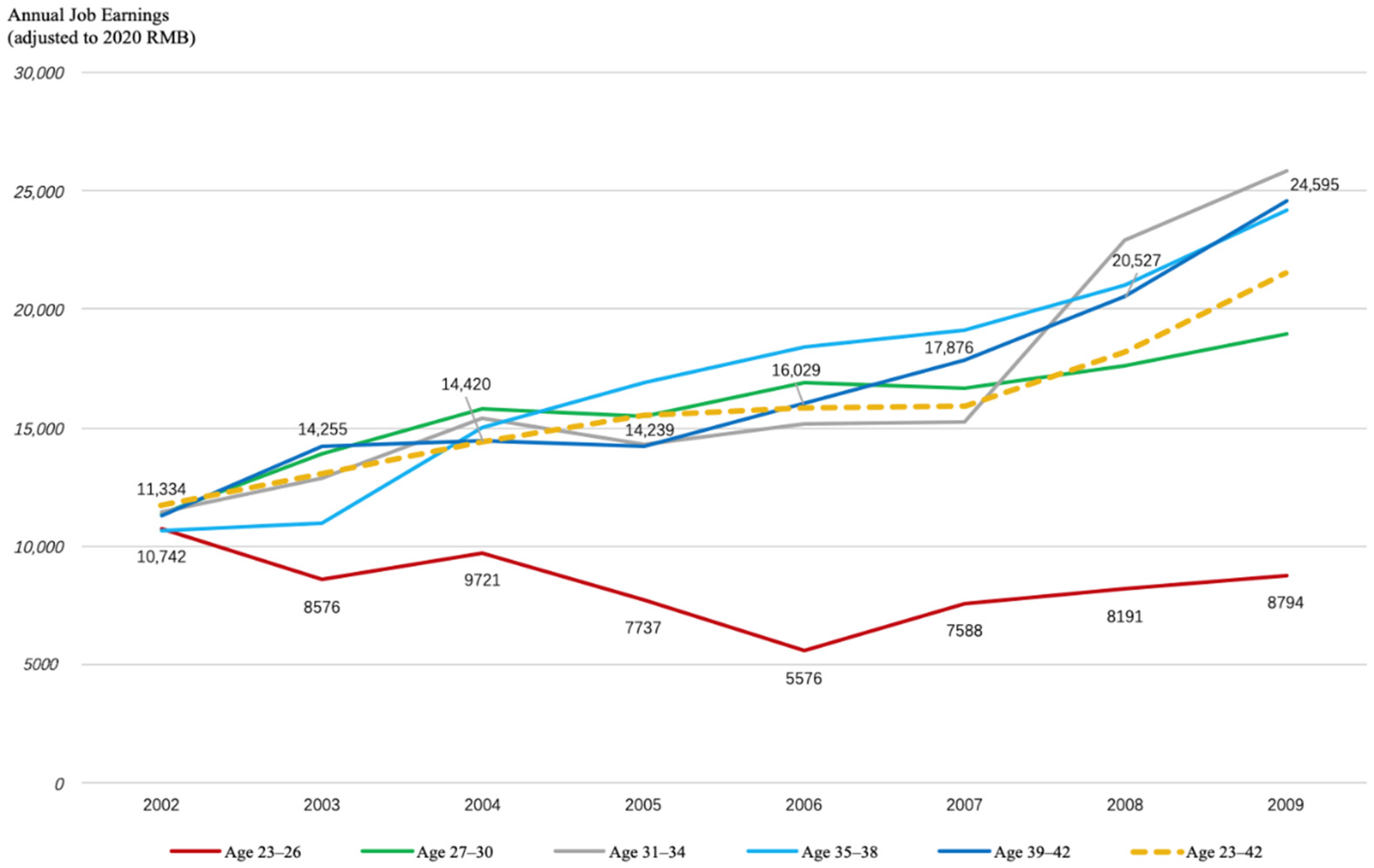
Figure 1. BA–HS wage gaps, sample mean and by age group (males only), 2002–2009.
Sustainability 14 16917 g001
Figure 2. Number of graduates from 4-year higher education institutions, 1982–2008.
Sustainability 14 16917 g002
Figure 3. Age-group-specific and aggregate relative supply index for BA- vs. HS-educated labor, 2002–2009.
Sustainability 14 16917 g003
Figure 4. Age-group-specific and aggregate relative supply index for BA- vs. HS-educated labor for selected age groups, 2002–2025.
Sustainability 14 16917 g004
Table 1. BA–HS Wage Gaps (in 2020 Chinese yuan), by Age Group, By Year (Males Only).
20022003200420052006200720082009
Age 23–2610,7428576972177375576758881918794
Age 27–3011,35813,90415,83415,45316,88716,68517,63918,987
Age 31–3411,42112,89815,43114,31615,18115,27222,90725,838
Age 35–3810,65610,99415,00816,89418,39519,11021,04924,151
Age 39–4211,33414,25514,42014,23916,02917,87620,52724,595
Sample Mean (Age 23–42)11,75413,07814,42915,54815,86215,95518,22221,497
Number of observations: 52,483
Notes: Sample includes men born in 1960–1986 and who were 23–42 years old at the time of survey, and excludes men who were retired, disabled, or enrolled in school at the time of survey. Sample includes men with zero earnings due to unemployment or no-pay jobs. Wage gaps are calculated as the difference in mean annual employment income (inflated to 2020 Chinese yuan value) between BA- and HS-educated male labor in the indicated age group and survey year.
Table 2. BA–HS wage gaps (in natural logarithm form), by age group, by year (males only).
20022003200420052006200720082009
Age 23–260.4550.3640.4360.4050.2340.3360.3230.311
Age 27–300.6210.5950.6160.5840.6250.6020.5930.595
Age 31–340.4880.5050.6400.4570.4640.4570.5710.589
Age 35–380.4950.4630.5660.5780.5140.5450.6030.574
Age 39–420.5020.5560.5570.5380.5090.5240.6250.610
Sample Mean (Age 23–42)0.5260.5330.5850.5420.4840.4930.5410.561
Number of observations: 46,972
Notes: Sample includes men born in 1960–1986 who were 23–42 years old at the time of survey, and excludes men who were retired, disabled, or enrolled in school at the time of survey. Sample only includes men with positive earnings from employment. Wage gaps are calculated as the difference in mean log annual employment income between BA- and HS-educated male labor in the indicated age group and survey year.
Table 3. Age-group-specific and aggregate relative supplies of BA- vs. HS-educated labor by year.
Measures of Relative Supply of BA/HS LaborSurvey Year
20022003200420052006200720082009
Age-group-specific relative supply:
Age 23–260.1300.1500.1640.1790.2090.2560.3310.407
Age 27–300.0830.0890.0940.1130.1300.1500.1640.179
Age 31–340.0880.0810.0770.0780.0830.0890.0940.113
Age 35–380.0820.0980.0970.0910.0880.0810.0770.078
Age 39–420.0500.0480.0470.0580.0820.0960.0970.086
Aggregate relative supply (aged 23–42):
with perfect substitution across age groups0.0890.0910.1010.1140.1300.1470.1620.170
with imperfect substitution across age groups0.1150.1230.1350.1540.1750.1960.2110.228
Table 4. Decomposing BA–HS wage gaps into age-group-specific and aggregate relative labor supply, aggregate relative labor demand, and age effects (males only).
Model 1Model 2Model 3
Age-group-specific relative supply of BA-educated labor−0.199***−0.193***−0.195***
(0.005) (0.005) (0.005)
Aggregate relative supply of BA-educated labor with perfect substitution across age groups---−4.904***---
---(0.237) ---
Aggregate relative supply of BA-educated labor with imperfect substitution across age groups------−0.560***
------(0.049)
Annual temporal trend---0.593***0.095***
---(0.027) (0.008)
Age effects (Age 23–26 as base):
Age 27–300.411***0.413***0.412***
(0.005) (0.005) (0.005)
Age 31–340.395***0.398***0.397***
(0.006) (0.006) (0.006)
Age 35–380.398***0.403***0.401***
(0.006) (0.006) (0.006)
Age 39–420.270***0.274***0.274***
(0.007) (0.007) (0.007)
Including survey year fixed effectsYESNONO
Number of observationsN = 46,972
R-square0.5100.7810.890
Notes: *** indicates significance at the 0.01% level. Standard errors are in parentheses. Models are fit by ordinary least squares to the age-group by year BA–HS wage gaps in natural logarithm form shown in Table 2.
Table 5. Decomposing BA–HS wage gaps into age-group-specific and aggregate relative labor supply, aggregate relative labor demand, and age effects (female and male workers).
Model 1Model 2Model 3
Age-group-specific relative supply of BA-educated labor−0.156***−0.180***−0.163***
(0.005) (0.005) (0.005)
Aggregate relative supply of BA-educated labor with perfect substitution across age groups---−6.894***---
---(0.106) ---
Aggregate relative supply of BA-educated labor with imperfect substitution across age groups------
---
−0.833***
---(0.091)
Annual temporal trend---0.740***0.079***
---(0.012) (0.008)
Age effects (age 23–26 as base):
Age 27–300.364***0.357***0.363***
(0.005) (0.006) (0.006)
Age 31–340.369***0.352***0.369***
(0.006) (0.007) (0.006)
Age 35–380.371***0.352***0.372***
(0.006) (0.006) (0.006)
Age 39–420.258***0.234***0.258***
(0.007) (0.007) (0.007)
Including survey year fixed effectsYESNONO
Number of observationsN = 72,494
R-square0.4410.7620.854
Notes: *** indicates significance at the 0.01% level. Standard errors are in parentheses. Sample includes individuals born in 1960–1986 who were 23–42 years old at the time of survey, and excludes those who were retired, disabled, or enrolled in school at the time of survey. Models are fit by ordinary least squares to the age-group by year BA–HS wage gaps in natural logarithm form for female and male workers. All the labor supply measures are adjusted by gender weights to account for differences in labor force participation rates and average hours worked between females and males.
Table 6. Age-group-specific and aggregate relative supplies of BA- vs. HS-educated labor by year, 2010–2025.
Survey Year
2010201120122013201420152016201720182019202020212022202320242025
Age-group-specific relative supply:
Age 23–260.4540.4690.4680.4730.4870.5190.5520.5900.6320.6610.6780.7040.7450.8040.8910.989
Age 27–300.2060.2510.3310.4140.4540.4430.4240.4120.4260.4300.4340.4640.4880.5170.5520.610
Age 31–340.1290.1490.1590.1690.1950.2370.3120.3840.3850.3890.3900.3820.3800.3850.4110.440
Age 35–380.0830.0890.0920.1110.1270.1460.1570.1660.2150.2330.3070.3840.4210.4220.4100.409
Age 39–420.0880.0900.0950.0970.0980.1010.1040.1060.1140.1160.1240.1320.1520.1850.2440.304
Aggregate relative supply with imperfect substitution across age groups:
Age 23–420.2660.2900.3170.3540.3880.4260.4670.4990.5490.5670.5960.6320.6730.6990.7540.833
Notes: BA-educated labor in the 23–26 age group for years 2022–2025 uses projected number of BA graduates in 2022–2025 that are predicted using number of newly enrolled students in 4-year colleges in 2018–2021 adjusted by a graduation probability for each year. All the relative supply measures are calculated the same way as those in Table 3.
Table 7. Predicted wage gaps for selected years.
2009
(as Baseline)
2013201820222025
Wage GapΔ Wage GapPredicted Wage GapWage Gap Using CHIP DataΔ Wage GapPredicted Wage GapWage Gap Using CHIP DataΔ Wage GapPredicted Wage GapΔ Wage GapPredicted Wage Gap
Age 23–260.3110.040.3240.336−0.050.2950.302−0.100.280−0.360.201
Age 27–300.595−0.190.4820.479−0.330.3990.375−0.280.428−0.550.267
Age 31–340.589−0.030.5730.565−0.400.3530.387−0.410.349−0.650.207
Age 35–380.574−0.010.5670.573−0.290.4100.401−0.810.108−0.920.048
Age 39–420.6100.040.6370.606−0.060.5720.542−0.090.556−0.580.257
Age 23–420.561−0.130.4880.497−0.260.4140.403−0.380.348−0.650.196
Notes: Column 1 under each year presents estimated changes in age-group-specific wage gaps from the corresponding baseline wage gaps in 2009; Column 2 lists predicted wage gaps for selected years; Column 3 shows the difference between mean log annual labor income for BA- and HS-educated male workers in specific age groups estimated using the CHIP 2013 and CHIP 2018 datasets.
Publisher’s Note: MDPI stays neutral with regard to jurisdictional claims in published maps and institutional affiliations.